Munich Personal RePEc Archive
Re-evaluating the success of the EPA’s
33/50 program: evidence from facility
participation
Martina, Vidovic and Neha, Khanna
Rollins College, Binghamton University
16 August 2010
1
Running Title: Re-evaluating the Success of the EPA's 33/50 Program
Re-evaluating the Success of the EPA's 33/50 Program: Evidence from Facility Participation
Martina Vidovic+
Department of Economics, CSS 180 Rollins College, 1000 Holt Avenue
Winter Park, FL 32789
Email: [email protected]; Phone: 407-691-1380
and
Neha Khanna*
Department of Economics and Environmental Studies Program, LT 1004 Binghamton University, P.O. Box 6000
Binghamton NY, 13902-6000
Email: [email protected], Phone: 607-777-2689
+
We thank Catherine Miller of Hampshire Research for providing us data on Program participation. Michael Delgado provided comments on an earlier draft. All errors are ours.
*
2
Abstract
Using previously unavailable data, we examine facility participation in the 33/50 Program
and its effect on aggregate and toxicity weighted emissions between1991 and 1995 for a sample
of facilities whose parent firms committed to the Program. By focusing on individual facilities
we avoid the biases created by aggregating emissions across facilities. We find that while more
polluting facilities within a firm were more likely to participate, even when we account for the
toxicity of emissions, across firms there is no evidence of greater participation by facilities with
higher emissions. Although emissions of the 33/50 chemicals fell over the years, we find that
participation in the Program did not lead to the decline in the 33/50 releases generated by these
facilities.
Keywords: Toxic Release Inventory; program participation; program evaluation, GMM, dynamic panel
3
1. Introduction
In the early 1990s the United States Environmental Protection Agency (EPA) initiated a
series of voluntary agreements under which firms pledge to reduce their emissions of pollutants
otherwise not regulated directly. The 33/50 Program was the first of these voluntary initiatives.
Inaugurated in 1991, its goal was to reduce the releases and transfers of 17 high priority
chemicals by 33% by 1992, and by 50% by 1995, compared to their 1988 levels [7]. Under this
Program, the EPA sent letters to eligible company Chief Executive Officers eliciting their
participation in the Program. Roughly 1,300 companies responded with a clear commitment to
participate. These firms accounted for over 60% of the 1988 emissions of the 33/50 chemicals
[7]. Emissions data reported to the EPA’s Toxic Release Inventory (TRI) show that over the life
of the Program, 1991-1995, releases and transfers of the 17 targeted chemicals fell by 47%, and
according to the EPA, the ultimate goal of the Program, 50% reduction in emissions relative to
1988 levels, was achieved in 1994, a year ahead of schedule [7].
Several studies evaluate the success of the Program and the results of this literature are
not conclusive. Those studies that argue that the Program was successful analyze only the
chemical sector [13], use a small subset of firms that also adopted Total Quality Environmental
Management which is another voluntary activity [17], or find that participation in the Program
led to a reduction in firm emissions only in the first year of the Program, 1991 [12].
Gamper-Rabindran [8] and Vidovic and Khanna [20] analyze firms from all industry sectors and find
participation in the Program had no effect on the emissions of the targeted chemicals. Vidovic
and Khanna [20] conclude that the reduction in the emissions observed by the EPA was the result
of an independent trend rather than a direct consequence of the Program.
4
commitment and examine the impact of participation in the 33/50 Program on facility emissions
using a sample of facilities whose parent companies committed to the Program. According to the
Program design, a parent company was recognized as a participant even if only one of its
production facilities participated in the Program. This allowed facilities to free ride on
reductions achieved by a subset of production plants, thus potentially diluting the impact of
Program participation at the firm level. For example, the abatement effort of a single facility
might decrease overall firm emissions despite the fact that no other facility belonging to the
parent firm reduced emissions. Conversely, it is possible that the pollution abatement efforts of
some facilities are outweighed by the increase in emissions of other facilities owned by the same
firm so that overall firm emissions increase. Yet, such firms would be counted as participants in
the 33/50 Program. Thus, a firm level analysis has potential biases that work against an accurate
evaluation of the Program, and it is not surprising that the results of the firm level analyses that
dominate the literature are mixed. By using facility level information regarding commitment to
the Program we are able to rule out such possible free riding across facilities owned by the same
firm. Therefore, we are better able to assess the impact of participation in the Program using our
facility level data, even though the Program was operational at the firm level.
Only three other studies explicitly consider facility participation. Due to lack of data,
Khanna and Vidovic [14] and Gamper-Rabindran [8] incorrectly assume that all facilities
belonging to a parent firm that committed to the Program participated. Bi and Khanna [5] use
the newly available data on facility participation but include all facilities in their analysis,
regardless of their parent firm’s participation status. Using a sample of 2,034 facilities that
belong to 197 publicly owned parent firms that participated in the Program, we analyze the
5
using a panel data Generalized Method of Moments (GMM) framework to account for dynamic
adjustment in facility emissions. We find that while more polluting facilities within a firm were
more likely to make commitments to reduce the releases and transfers of the targeted chemicals,
participation in the Program by itself is not associated with a significant decline in emissions.
This result is consistent with our earlier analysis of firm level data [20] but contrary to the results
of Khanna and Damon [13], among others.
2. Incentives for participation in the 33/50 Program and hypothesis tested
2.1. Incentives for participation
The EPA emphasized that the 33/50 Program was appealing to firms because participants
received public recognition through the media and certificates of recognition from the EPA. The
literature on voluntary abatement programs suggests four mechanisms that motivate firms to
participate: green marketing [3, 4, 13, 20], regulatory pressure [12, 13, 15, 18, 19, 20], interest
group pressure [12, 17], and firm specific characteristics such as its size [3, 19, 20], financial and
asset position [3, 12, 17], emissions profile [3, 12, 13, 20] and proclivity to participate in other
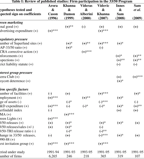
voluntary abatement programs [3, 13]. Table I summarizes the literature on firm participation in
terms of the main hypotheses, variables used to test each hypothesis, expected sign on variable
coefficients and the actual sign and the statistical significance of the coefficients obtained.
The incentives for facility participation, explored by Khanna and Vidovic [14],
Gamper-Rabindran [8] and Bi and Khanna [5], are very similar to those for firm participation. However,
because individual facilities do not typically interact directly with the final consumer, the
incentives created by green marketing opportunities ([4]) are unlikely to operate at the facility
6
may be even greater for facilities. For example, facilities located in counties classified as being
out of attainment with the National Ambient Air Quality Standards (NAAQS) may be more
likely to participate in order to improve their environmental performance and avoid more
stringent mandatory regulation in the future [9]. Indeed Bi and Khanna [5] find facilities located
in non-attainment counties are more likely to participate. All three facility level studies examine
the participation incentives created by the National Emission Standards for Hazardous Air
Pollutants but only Khanna and Vidovic [14] find that facilities with higher ratios of the HAPs to
33/50 emissions are more likely to participate. Bi and Khanna [5] and Gamper-Rabindran [8]
find that plants that were inspected more frequently for compliance or penalized for
non-compliance with Clean Air Act (CAA) regulations were more likely to join the 33/50 Program.
Pressure from local communities and non-governmental organizations may create
additional incentives for participation. Plants may participate in voluntary programs in order to
deter environmentally conscious consumers and environmental interest groups from lobbying for
increased regulation [11, 15, 12]. This threat of tighter regulation is more likely to be a motive
for facility participation in states with higher membership in environmental interest groups such
as the Sierra Club, or in states with Congressional representatives that have a track record of
voting in favor of environmental initiatives [10, 15, 12]. Bi and Khanna [5] test the association
between the probability of facility participation and the home state’s representatives’
environmental rating as published by the League of Conservation Voters (LCV) as well as the
state per capita membership rate in the Sierra Club, but find that facilities located in states with
higher membership rates in the Sierra Club are less likely to participate. In addition, facilities
located in neighborhoods with a higher willingness to pay for environmental amenities and with
7
voluntary agreements. Khanna and Vidovic [14] and Bi and Khanna [5] find facilities located in
counties with a higher median income are more likely to join the Program. On the other hand
there is no evidence that voter participation rates or the socio-economic and demographic
composition of a county have an effect on a facility’s participation decision [14, 8].
Based on the current literature, we anticipate that larger, more polluting facilities, as well
as facilities that emitted a larger share of their parent firm’s 33/50 emissions and whose parent
firms were invited in the first wave of invitations are more likely join the Program. Facilities
emitting a larger absolute quantity of 33/50 releases or a larger share of their parent company's
33/50 emissions may be been more likely to join the Program since they face a greater potential
for emission reduction. Similarly, facilities whose parent companies were invited in the first
wave may be more likely to participate either because they had higher 33/50 emissions or
because they received greater outreach by the EPA.1
To the extent that facilities may wish to mitigate the cost and stringency of current and or
future mandatory regulation, we anticipate that facilities with higher total TRI emissions, a larger
number of government inspections and enforcement actions under the CAA, and facilities that
emit a larger share of 189 HAPs among all TRI chemicals may be more likely to join the 33/50
Program. We also expect to find that facilities located in regions with tougher air pollution
policies and greater community environmentalism will have a higher probability of participation.
For that reason, we presume facilities located in states with a larger per capita membership in
Sierra Club and facilities located in counties with a greater propensity for collective action may
be more likely to participate. Similarly, facilities located in counties designated to be out of
attainment with NAAQS and facilities located in states with higher LCV scores may fear tougher
1
8
regulation in the future and be more likely to self-regulate to reduce regulatory pressure.
2.2. Hypothesis tested
Our main hypothesis is that facilities that committed to the Program lowered their
emissions of the 17 targeted chemicals as a result of joining the Program. We presume that a
facility's emissions of the 33/50 chemicals are determined by its participation in the Program and
many of the same factors that shape its participation decision such as the percentage of HAPs in
total TRI emissions, number of inspections and enforcement actions, LCV score and per capita
membership in Sierra Club in the facility's home state, number of air pollutants the facility's
home county is in non-attainment with the CAA, and voter participation rates in the facility's
home county. Additional controls include socio-economic and demographic characteristics of a
facility's home county. We anticipate that facilities that expect larger potential liabilities under
mandatory regulation and facilities that experience greater pressure from constituents and
non-governmental environmental groups will have lower 33/50 emissions.
The Program goals were formulated in terms of aggregate emissions. This gave firms an
incentive to focus their efforts on the chemicals with the lowest marginal abatement costs rather
than the most toxic chemicals. From a public health perspective, however, the relative toxicity
of the chemicals is important. Even if the aggregate emissions of the targeted chemicals declined
as a result of the Program, the overall toxicity of the emissions need not have declined in tandem,
especially because firms could reduce emissions of only a subset of the Program chemicals and
could potentially substitute more toxic chemicals for less toxic ones. Therefore, in addition to
analyzing aggregate emissions, we also analyze the impact of Program participation on toxicity
9
3. Methodology
We examine the incentives for participation in the 33/50 Program and the impact of the
Program on emissions of the targeted chemicals for a sample of facilities whose parent firms
committed to the Program. The EPA sent letters of invitation to the Chief Executive Officers of
parent companies and not to individual facilities [7], and we assume that the decision to
participate was first made by the parent firms and then extended to their facilities.
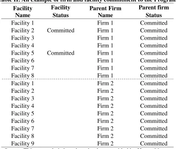
Our approach is motivated by the data made available to us by Hampshire Research. As
Table II shows, our data include parent companies that committed to the Program and some but
not all of their facilities also committed, and parent companies that committed but none of their
facilities committed.2 If none of the facilities committed but the parent company did commit, the
decision to participate could not have been driven by the decision at the facility level and was
probably made by the parent company. Assuming that all commitments were credible and made
with the intention of meeting their stated goals, a company that joined the Program would have
to reduce its emissions, even if none of its facilities specifically joined the Program. This would
imply that when a parent firm committed to the Program, it automatically jointly committed all
of its facilities to the Program. In this sense, all nine facilities belonging to Firm 2 in Table II are
participants in the 33/50 Program, even though no individual facility made a specific
commitment to join the Program. Thus, in the case where the parent company committed and
none of the facilities committed, it does not make sense to model these facilities as
non-participants while ignoring the firm decision. We prefer to consider these nine facilities as not
having made any specific commitment over and above the firm’s decision to participate in the
Program. This distinguishes these facilities from Facility 2 and Facility 5 of Firm 1, both of
which made a specific commitment to the EPA. Note that the EPA regarded both Firms 1 and 2
2
10 as participants and did not distinguish between them.
For this reason we assume that the decision to participate in the Program was made at the
company level, and conditional on the parent firm’s participation decision, individual facilities
made additional commitments to reduce their emissions and participate in the Program.
Therefore, our estimation strategy is threefold: we first model the firm’s participation decision,
and using data only on facilities that belong to firms that participated in the Program, we model
the facility’s participation decision. Finally, we evaluate the facility’s emissions conditional on
its participation decision. To test the sensitivity of our results we follow Bi and Khanna [5] and
also model the facility participation decision independently of the firm’s decision using the entire
universe of facilities eligible to participate in the Program. In this case, the nine facilities
belonging to Firm 1 in Table II are no different from facilities belonging to a parent firm that did
not participate in the Program.
4. Empirical model
A facility's expected net benefit from participation in the Program, , is given by
(1)
where is a vector of covariates, is a vector of coefficients, and We do not
observe , only whether the facility participated or not. That is, we observe , a
dichotomous variable equal to 1 if the expected net benefit is positive and 0 otherwise.
Furthermore, is only observed for a subset of facilities whose parent firms participated in the
Program. That is is observed if and only if is equal to 1, where is a dichotomous
variable equal to 1 if the parent firm's expected net benefit from participation is positive and 0
11
(2)
where is a vector of covariates, is a vector of coefficients, and This leads to
a bivariate probit model with sample selection.
We estimate and in Eqs. (1) and (2) simultaneously using maximum likelihood
methods and assuming that and are distributed bivariate normal with means and standard
deviations as specified above, and that If the facilities are randomly
selected to the sample and consistent estimates of can be obtained by estimating model (1)
with an ordinary probit regression. After estimation, a simple likelihood ratio test (or Wald test)
can be used to test the null hypothesis that .
For the model to be identified there should be at least one right hand side variable that
appears in the selection equation (Eq. 2) but does not appear in the outcome equation (Eq. 1). In
our case the selection equation includes firm level variables. These are a final good dummy,
change in aggregate 33/50 emissions prior to the start of the Program, ratio of HAPs to TRI
emissions, ratio of 33/50 emissions to TRI emissions, number of Superfund sites for which a
firm is a Potentially Responsible Party (PRP), number of inspections and enforcement actions
against a parent firm’s facilities, Sierra Club membership and the LCV score averaged across a
firm’s facilities, and firm specific factors such as age of assets and R&D expenditure. The first
invitation group dummy is the only variable common to both equations.
Given that we have data on a panel of I facilities and firms over T years, we would like to
use panel data methods to estimate Eq. (1). However, the corresponding panel data estimator is
not available and we use a pooled cross section estimator but adjust standard errors for
intra-panel correlation.3
3
12
Facility emissions at time t, , are determined by a set of facility specific factors, ,
and the facility's participation decision, ! , as
! " # $ (3)
where is a vector of coefficients, " is a scalar coefficient, # is a fixed effect and
$ % includes facility specific factors that determine its emissions in any year, such
as its level of output, operational decisions and the organizational culture. Such detailed facility
level information is not available in the public domain. Furthermore, changes in the level of
output and adoption of new technology occur slowly over time and are generally unobserved. To
account for such effects and the lack of detailed facility information we include the lagged values
of facility emissions on the right hand side of equation (3). This leads to a dynamic specification
for , as
& ' ( ( ! " # $ (4)
where ( includes facility and parent firm specific factors for which information is available.
As facility emissions are determined by many of the same factors that affect facility
participation in the Program, ! is endogenous in Eq. (4). We use the predicted probability of
participation for each facility for each year from Eq. (1), ) * , which is a cumulative
distribution function, as an instrument for the facility's participation decision in Eq. (4).
Again, we would like to exploit the panel structure of the data. Applying the fixed effects
estimator to Eq. (4) will result in a dynamic panel data bias as & is correlated with the error
term. Arellano and Bond [1] suggest transforming the model by taking first differences to
eliminate the fixed effects, and then estimating it using instrumental variable techniques where
the second and higher lags of the endogenous variables in levels are used as instruments.
13
However, lagged levels are often poor instruments for first differences. Arellano and Bover [2]
and Blundell and Bond [6] show that this problem can be alleviated by estimating a system of
equations which includes the original equation in levels and uses lagged differences as
instruments. A secondary advantage of this system GMM estimator is that it can also
accommodate models with time invariant regressors.
We apply system GMM to Eq. (4). The estimator rests on the strong assumption that
lagged values of the dependent variable and changes in the error term are uncorrelated. Although
first order autocorrelation is expected, we examine the validity of this assumption by testing for
the presence of second order autocorrelation. We estimate robust standard errors using the
two-step version of the system GMM estimator with a finite-sample correction [21].4
The rank and order conditions for identification of the parameters in Eq. (4) require that
we have some variables in Eq. (1) that are hypothesized to influence facility participation but are
otherwise uncorrelated with the facility emissions. We include three variables in Eq. (1) that are
not in Eq. (4): first invitation group dummy, change in facility 33/50 emissions between 1988
and 1990, and the percentage of the parent firm's 33/50 releases emitted by a facility.
5. Data description
We draw upon several data sources. Hampshire Research provided us with the list of
firms invited to participate in the 33/50 Program, their participation status, and information about
when the firm was contacted by the EPA. For the firms that participated in the Program, they
also provided us with a list of facilities and their participation status. We obtained data on
emissions of the 33/50 chemicals, total TRI releases, HAP releases, names and Dun and
4
14
Bradstreet numbers of parent firms, and facility SIC codes and locations from the TRI
(www.rtknet.org/new/tri). Information on the number of inspections and enforcement actions
under the CAA is from the Integrated Data for Enforcement Analysis database
(www.epa-echo.gov/echo/index.html); county nonattainment status with the CAA is from the EPA's Green
Book (www.epa.gov/oar/oaqps/greenbk). LCV scores are from various National Environmental
Scorecards published annually by the League of Conservative Voters (www.lcv.org). The Sierra
Club provided us with the data on its state per capita membership while Election Data Services
provided county level voter participation rates. Firm level financial data are from the Standard
and Poor's Compustat database and the information on Superfund Site responsibility is from the
CERCLIS database (http://cfpub.epa.gov/supercpad/cursites/srchsites.cfm). County
socio-economic data is from the 1990 Census.
We define facility emissions of the 33/50, HAP and TRI chemicals as annual releases to
air, surface water, land, and underground injection plus offsite transfers to treatment, storage and
disposal. Toxicity weighted 33/50 emissions are pounds of emissions multiplied by the toxicity
weights used in the EPA's Risk Screening Environmental Indicators
(http://www.epa.gov/oppt/rsei/). We weight the air releases of each of the 17 chemicals by their
inhalation toxicities and the emissions to other media by oral toxicities. Firm emissions are the
sum of the emissions for all facilities reporting to each parent company in each year. We define
the change in the pre-Program 33/50 releases as the emissions in 1990 minus the emissions in
1988. We use total facility TRI emissions to capture facility size.
The state LCV score is an average of the rating assigned to the elected officials in the
Senate and the House of Representatives by the LCV based on their voting record on
15
commitment to environmental protection, while a score of 0 shows a consistent voting pattern
against conservation and environmental health and safety protection. The county non-attainment
status is the count of pollutants for which a whole or a part of the county has been designated by
the EPA to be out of attainment with the NAAQS. The EPA will designate the county to be in
nonattainment whenever air pollution levels persistently exceed the NAAQS for six pollutants:
ozone, lead, carbon monoxide, sulfur dioxide, nitrogen dioxide and particulate matter. We define
the firm level LCV score, per capita membership in Sierra Club, number of enforcements and
inspections as the average across all plants owned by a parent firm.
We represent the propensity for collective action by the fraction of the voting age
population registered to vote in the 1992 Presidential elections in a facility’s home county.5
Socio-economic and demographic characteristics of the county in which a facility is located
include the fraction of African-American population, the percentage of population with at least a
bachelor's degree, median household income, the percentage of population below poverty, and
the percentage of children up to 5 years of age. Additional control variables include population
per square mile and dummy variables for the facility 2 digit primary SIC codes.
To construct our sample we first searched the TRI to identify facilities that emitted a
positive amount of 33/50 chemicals in 1988, 1989 or 1990. This resulted in 16,550 facilities in
the continental United States. We successfully matched 13,734 facilities to their parent
companies by either parent firm name or Dun and Bradstreet number.6 Since we model facility
participation conditional on the parent firm’s decision, we use an unbalanced panel of 368
publicly owned firms represented in the Standard and Poor’s Compustat database of which 197
5
North Dakota and Wisconsin do not report voter registration. For these two states, we use the ratio of voter turnout to voting age population.
6
16
firms participated in the Program and 171 did not participate over the period 1991 – 1995.7 To
evaluate facility emissions and participation in the Program, we use a subset of 2,034 facilities
that belong to these 197 participating firms. Out of the 2,034 facilities, 126 participated and
1,908 did not participate in the Program. Most facilities in our sample reported to the TRI for at
least three years between 1991 and 1995.
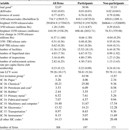
Tables III and IV summarize our data for 1990. On average, participating firms have
higher aggregate and weighted 33/50 emissions as well as release intensity per unit of sales
relative to non-participants. They have a larger number of facilities, face a larger number of
inspections and enforcement actions and are a PRP for a greater number of Superfund sites.
Compared to non-participants they also reduced emissions of the Program chemicals by a larger
amount between 1988 and 1990 and a larger fraction was included in the first invitation group.
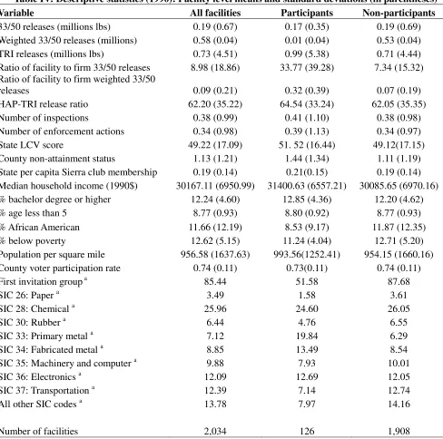
At the facility level, participating facilities have lower aggregate and toxicity weighted
33/50 emissions compared to non-participating facilities. Compared to non-participants,
participants have higher total TRI emissions, face a larger number of inspections and
enforcement actions and a larger number of them are located in counties that are in
nonattainment with a greater number of pollutants, as well as counties characterized by higher
median household income and lower percentage of African American population. 85% of the
facilities in our sample are owned by firms invited to participate first; however, a larger
percentage of these facilities are non-participants.
Comparing emissions in 1991 to 1995, we find that the 197 participating firms in our
sample reduced their emissions of the 33/50 chemicals by 42.4% relative to 1991 compared to
43.6% by the non-participating firms. If we consider the entire universe of firms for which the
EPA provided us with information (i.e., including non-publicly traded firms contacted by the
7
17
EPA, and firms located in Hawai’i, Alaska and Puerto Rico) the 1287 participating firms
decreased their 33/50 releases by 41.8% compared to 30.4% by the 6143 non-participating firms.
At the facility level we find that the 126 participating facilities in our sample that belonged to
participating firms decreased their 33/50 releases by 46.3% compared to the 42.8% decline
achieved by the 1908 non-participating facilities. This compares to the 52.3% reduction
achieved by 1060 participating facilities and 39.5% reduction by 5751 non-participating facilities
in the entire EPA dataset of participating firms. Given these statistics, it is possible that the
sample of publicly owned firms and their facilities that we use in our benchmark analysis is not
representative. For this reason, we also use a secondary and much larger sample of facilities for
which the summary statistics on emissions reductions are much closer to the universe of firms
and facilities for which the EPA provided us with information (see section 6.4 for details).
6. Results and discussion
6.1. Facility participation in the Program
We first examine the incentives for facility participation in the 33/50 Program. We have a
non-random sample of 2,034 facilities whose parent firms committed to the Program leading to
9,701 facility-year observations. The facility participation results obtained from simultaneously
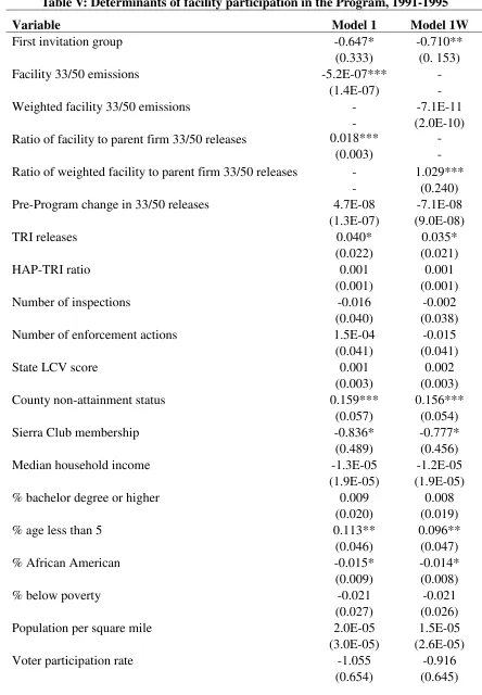
estimating Eqs. (1) and (2) by maximum likelihood are presented in Table V. We include on the
right hand side aggregate 33/50 emissions in Model 1 and the toxicity weighted 33/50 emissions
in Model 1W. All time varying variables are lagged by one year relative to the year in which a
facility participation decision is measured.8 We control for eight most representative industry
groups based on two-digit SIC codes. Table A1 in the Appendix presents the results of the
8
18
selection equation on firm participation in the Program.9
In both models in Table V we find that facilities that account for a larger proportion of a
parent firm’s aggregate and toxicity weighted 33/50 emissions were more likely to participate.
On the other hand, facilities with greater 33/50 emissions were less likely to participate while the
level of toxicity weighted emissions does not seem to have a statistically significant impact on a
facility’s participation decision. The coefficient on the variable measuring the change in
aggregate facility emissions between 1988 and 1990 is not statistically significant indicating that
facility participation was not driven by reductions in emissions achieved prior to the start of the
Program. In addition, we find weak evidence that larger facilities as measured by the aggregate
TRI emissions were more likely to join the Program.
In terms of regulatory pressure, the coefficient on county nonattainment status is
statistically significant and positive indicating that the Program attracted facilities located in
counties in which a larger number of the regulated pollutants that were out of attainment with
NAAQS. Surprisingly, the coefficient on Sierra Club membership is negative and statistically
significant at the 10% level indicating that facilities located in states with greater membership
rates in an environmental interest group were less likely to participate. Although there is
evidence that facilities located in counties with young children and a lower fraction of African
Americans were more likely to participate, community characteristics are generally not good
predictors of facility participation in the Program.
While the largest, most polluting firms invited in the first wave of invitations were more
likely to participate in the Program (Table A1), confirming the results of earlier studies of firm
9
19
participation, [3, 13, 20], we find that facilities belonging to these companies were less likely to
make additional commitments. The coefficients on the first invitation group dummy are negative
and statistically significant in both models.
For both models in Table V, the null hypothesis that the error terms in the outcome and
the selection equations are not correlated cannot be rejected at the 10% level of significance,
although in model 1W the p-value is less than 13%. This lack of evidence against the null
hypothesis at traditional levels of significance raises the question of whether we should model
facility participation conditional on the parent firm’s participation decision. Given the structure
of our data, and as discussed earlier in the context of Table 2, we feel that it is inappropriate to
model a facility’s participation decision ignoring the parent firm’s decision. Nonetheless, in
section 6.3 we test the sensitivity of our results by examining the association between facility
participation and facility emissions regardless of the parent firm’s participation decision.
6.2. Facility 33/50 emissions
To evaluate whether facility participation is associated with a decline in emissions we
analyze facility emissions over the life of the Program (1991-1995). We take the natural
logarithm of facility 33/50 emissions, toxicity weighted emissions and the TRI emissions. We
lag the number of inspections and enforcement actions by one year relative to the year in which
the dependent variable is measured. All other time varying variables are measured in the same
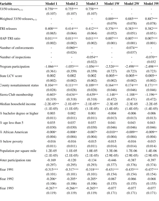
year as the dependent variable. The results of system GMM estimates are presented in Table VI.
In the Models 1-3 in Table VI, the dependent variable is the aggregate 33/50 emissions, while in
the Models 1W-3W, the dependent variable is the toxicity weighted 33/50 emissions. In all
20
statistically significant indicating that our instruments are valid from the perspective of these
tests. We found the fifth and the sixth lags to be a valid set of instrument for the lagged 33/50
emissions. We use the predicted probability of participation from the models in Table V as an
instrument for facility participation in the Program. All other variables act as their own
instruments.10 We include time dummies in all models.
In models 1 and 1W we presume that the number of enforcement actions or the number of
inspections affect the emissions of the 33/50 chemicals only indirectly through Program
participation and we do not include them on the right hand side. In models 2, 3, 2W and 3W, we
relax this assumption and account for the possibility that facilities with a poor environmental
record may reduce their emissions of the 33/50 chemicals to signal their environmental efforts.
The coefficient of most interest in Table VI is the coefficient on the Program participation
variable. In all models, this coefficient is negative and statistically significant indicating that
Program participation led to a decrease in both aggregate and toxicity weighted emissions for
facilities that have made additional commitments beyond their parent firm’s commitments. This
is in contrast to Gamper-Rabindran [8] but similar to Bi and Khanna [5].
While all the models shown in Table VI pass the Hansen’s J and Sargan tests, the crucial
test for the second order autocorrelation cannot be rejected even at the 10% level of significance
for the three models where the dependent variable is aggregate 33/50 emissions. This questions
the validity of the results for the first three models in Table VI. To account for this, we add the
second lag of the dependent variable to our original model. While the test for second order
autocorrelation is not statistically significant when the dependent variable is toxicity weighted
emissions, for consistency we add the second lag of the dependent variable to all models in Table
10
21
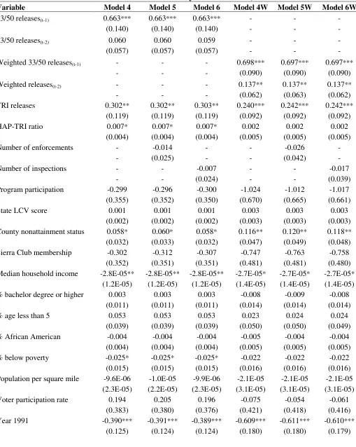
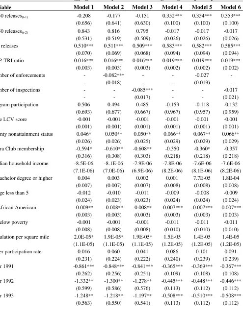
VI. The results are presented in Tables VII and VIII. In models 1-3 in Table VII, the left hand
side variable is aggregate 33/50 emissions while in models 1W-3W it is toxicity weighted 33/50
emissions. We treat the specification in Model 1 of Table VII as our benchmark model.
In all models in Table VII, the coefficient on the Program participation variable is not
statistically significant indicating that participation in the Program did not have a strong effect on
either the aggregate or toxicity weighted 33/50 emissions. Recall that in Table VI, the models for
weighted 33/50 releases pass all the tests for instrument validity and the coefficient on Program
participation is statistically significant in these models. Comparing the results for weighted
releases in Tables VI and VII shows that coefficient on Program participation is sensitive to
model specification and that the results should be interpreted with caution.
In Table VII, as in Table VI, we assume that a facility’s TRI releases and the HAP to TRI
release ratio are exogenously determined. However, HAPs were subject to regulation by the late
1990s and facilities that initiated reductions in HAPs would also reduce the 33/50 emissions even
in the absence of the Program. So, in Table VIII we treat these two variables as being
simultaneously determined with facility 33/50 emissions and therefore endogenous. We
instrument for these two variables using their own second and higher lags. Similar to the results
for our benchmark specification (model 1 in Table VII), the coefficient on Program participation
though negative is not statistically significant in any models in Table VIII, not even when the
dependent variable is toxicity weighted emissions (models 4W-6W). However, in all models in
Table VIII, the coefficients on the year dummies are negative and statistically significant
indicating that facilities reduced the emissions of the Program chemicals between 1991 and 1995
for reasons independent of the 33/50 Program and not directly accounted for in our model.
22
measured by the total TRI releases had higher aggregate and toxicity weighted 33/50 emissions.
Positive and statistically significant coefficients on the county nonattainment status and
HAP-TRI ratio indicate that facilities located in counties that were out of attainment with the CAA and
facilities that emitted a larger percentage of HAPs among all TRI chemicals had higher 33/50
emissions. Facilities located in counties with higher median household income had lower
aggregate and toxicity weighted emissions of the Program chemicals (Table VIII). On the other
hand, the coefficients on the number of enforcements and the number of inspections are not
statistically significant indicating that the anticipation of more stringent mandatory regulation did
not have an effect on emissions of the 33/50 Program chemicals.
6.3. Sensitivity analysis
Unlike our analysis that focuses on facilities that specifically committed to reduce
emissions in addition to the goals stated by their parent firms, Bi and Khanna [5] study
participation in the Program and its impact on the releases of Program chemicals for all facilities
eligible to participate, regardless of their parent firms’ decision. By assuming that the decision to
participate in the Program was made at the facility level, they are able to utilize a much larger
sample of facilities, including facilities owned by firms that are not publicly traded as well as
facilities that belonged to firms that did not commit to the Program.
To examine the sensitivity of our results, we explore the possibility that the participation
decision was made by facilities independently of parent firms. We use an unbalanced panel of
8,583 facilities eligible to participate in the Program over the period 1991 – 1995. Among these
facilities there are 792 participants and 7,791 non-participants. For this sample, participating
facilities reduced their emissions by 50.9% between 1991 and 1995 compared to 38.6% by the
23
system GMM using this larger sample of facilities, and ignoring the firm’s participation decision.
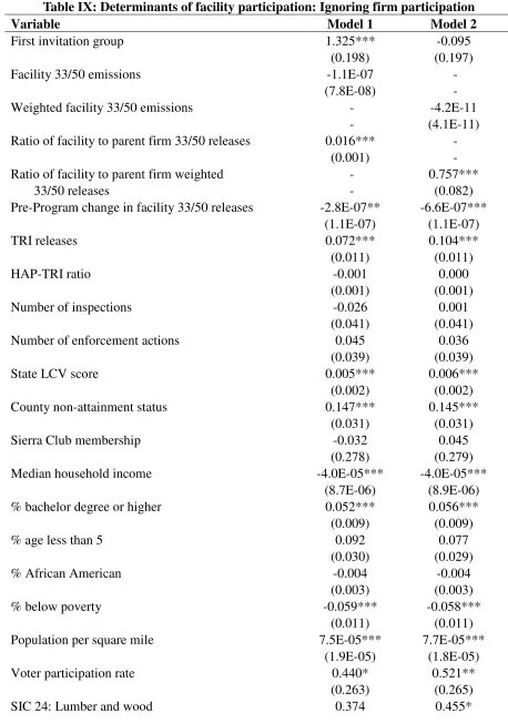
We estimate facility participation in the Program using a random effect probit model with
firms as cross sections. The results, shown in Table IX, are very similar to our benchmark results
reported in Table V. The main differences are that we now find some evidence to suggest that
facilities whose parent firms were invited first may have been more likely to participate (model
1) and the facilities that reduced 33/50 emissions in pre-Program years were more likely to join
the Program. Facilities located in states with higher LCV scores, facilities located in counties
that were out of attainment with CAA, and facilities located in counties with lower median
income as well as lower percentage of population below poverty were also more likely to
participate. We also find that facilities located in more densely populated counties, with a more
educated population and higher voter participation rates were more likely to join the Program.
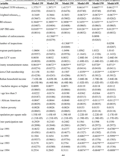
Tables X and XI show the results for aggregate and toxicity weighted facility emissions
of the 33/50 chemicals, respectively. All models include the second lag of the dependent variable
on the right hand side to account for the second order autocorrelation. We find that the
coefficient on facility participation in the Program is not statistically significant in any of the
models in Tables X and XI.
To assess how our results compare with Bi and Khanna [5], we follow their approach and
estimate the model of facility participation in the Program using a pooled probit and facility
emissions using a two step feasible GMM estimator.11 Regardless of how they instrument for
participation decision, Bi and Khanna find that the coefficient on Program participation is
negative and statistically significant. However, for our data, the coefficient on Program
participation is positive and statistically significant at the 10% level indicating that facilities that
11
24
participated in the Program may have increased rather than decreased emissions. For all other
variable coefficients we obtain qualitatively identical signs and significance. The only
exceptions are the coefficients on time dummies for which, unlike Bi and Khanna [5], we obtain
statistically significant and negative coefficients. These results are not shown here but are
available from the authors upon request.
Finally, we also estimate the models in Tables V, VI, VII and VIII using firms invited in
the first two invitation waves in 1991. The first invitation wave included the ‘top 600’ most
polluting firms and the second invitation wave included all firms that reported positive emissions
of any of the 17 targeted chemicals in 1988, 1989 or 1990. Innes and Sam [12] have argued that
for this set of firms, participation in the 33/50 Program was associated with a statistically
significant decline in emissions. The overwhelming majority of the firms in our benchmark
sample were invited in 1991: we lose only 37 facilities when we restrict ourselves to this smaller
sample of participating firms. Therefore, it is not surprising that our qualitative results are the
same as those reported in Tables V-VIII. These results are also available from the authors.
7. Conclusion
We examine the incentives for facility participation in the 33/50 Program and analyze the
impact of participation on facility level aggregate and toxicity weighted emissions over the
Program years, 1991-1995. Unlike others, we study the success of the Program at the facility
level using a sample of facilities that made commitments in addition to the overall commitments
made by their parent firms. These facilities communicated their participation decisions to the
EPA and thus identified themselves as the source of the potential emissions reduction to be
25
incentive to meet their stated goals and could not free ride on the efforts of other facilities
belonging to the same parent firm. So, if the 33/50 Program was successful in decreasing the
emissions of the 17 targeted chemicals, we are likely to find evidence for this in our sample.
Our analysis shows that most polluting facilities within a firm but not the most polluting
among all facilities across firms were more likely to join the Program. Unlike the literature on
firm participation, we do not find that a facility’s decision to participate was driven by the
incentive to preempt special interest groups from lobbying for tighter environmental regulation
and enforcement or to avoid later and more expensive penalties under mandatory regulation.
Thus, it seems that firms and facilities have different motives for joining voluntary programs.
More importantly, we find that participation in the Program did not have a direct effect on
facility emissions between 1991 and 1995, and that facilities may have reduced the emissions of
the Program chemicals for other reasons not directly accounted for in our model.
The currently published literature on the 33/50 Program, including our own earlier work,
analyzes the success of this voluntary pollution abatement program using firm level data on
participation and emissions. Two factors complicate a firm level analysis and lead to possible
aggregation biases. First, the EPA considered a parent firm as a participant even if only one of
its facilities participated in the Program. Second, while the emissions abatement under the
Program was executed by individual facilities, the EPA credited the decline in emissions to the
parent firm. The facilities that we classify as participants are facilities that made commitments to
the EPA and presumably were confident that they could bring about the necessary changes in
production to meet their environmental goals. That our results suggest that the observed
reduction in facility emissions was not correlated with facility participation unambiguously
26
References
[1] M. Arellano, S. Bond, Some tests of specification for panel data: Monte Carlo evidence and an application to employment equations, The Review of Economic Studies 58 (1991) 277-297.
[2] M. Arellano, O. Bover, Another look at the instrumental variable estimation of error components models, Journal of Econometrics 68 (1995) 29 – 51.
[3] S. Arora, T.N. Cason, Why do firms volunteer to exceed environmental regulations? Understanding Participation in EPA's 33/50 Program, Land Economics 72 (1996) 413-432.
[4] S. Arora, S. Gangopadhyay, Towards a theoretical model of voluntary over-compliance, Journal of Economic Behavior Organization 28 (1995) 289-309.
[5] X. Bi, M. Khanna, Re-assessment of the impact of EPA’s voluntary 33/50 program on toxic releases, Department of Agricultural and Consumer Economics at University of Illinois at Urbana Champaign working paper, 2009.
[6] R. Blundell, S. Bond, Initial conditions and moment restrictions in dynamic panel data methods, Journal of Econometrics 87 (1998) 111-143.
[7] Environmental Protections Agency (EPA), Office of Pollution Prevention and Toxics, 33/50 program: the final record, Washington DC (1999).
[8] S. Gamper-Rabindran, Did the EPA’s voluntary industrial toxics program reduce emissions? A GIS analysis of distributional impacts and by-media analysis of substitution, Journal of Environmental Economics and Management 52 (2006) 391-410.
[9] M. Greenstone, The impacts of environmental regulations on industrial activity: evidence from the 1970 to 1977 clean air act amendments and the census of manufacturers, Journal of Political Economy 110 (2002) 1175-1219.
[10] J.T. Hamilton, Taxes, torts, and toxics release inventory: congressional voting record on instruments to control pollution, Economic Inquiry 35 (1997) 745-762.
[11] I. Henriques, P. Sadorsky, The Determinants of an environmentally responsive firm: an empirical approach, Journal of Environmental Economics and Management 30 (1996) 381-395.
[12] R. Innes, A. Sam, Voluntary pollution reductions and the enforcement of environmental law: an empirical study of the 33/50 program, Journal of Law and Economics 51 (2008) 271 – 296.
[13] M. Khanna, L.A. Damon, EPA's voluntary 33/50 program: impact on toxic releases and economic performance of firms, Journal of Environmental Economics and Management 37 (1999) 1-25.
27
Economics at Binghamton University working paper, 2001.
[15] J.W. Maxwell, T.P. Lyon, S.C. Hackett, Self-regulation and social welfare: the political economy of corporate environmentalism, Journal of Law and Economics 63 (2000) 583-617.
[16] D. Roodman, How to do xtabond2: an introduction to “difference” and “system” GMM in Stata, Center for Global Development at Washington D.C. working paper, 2008.
[17] A.G. Sam, M. Khanna, R. Innes, Voluntary pollution reduction programs, environmental management, and environmental performance: an empirical study, Land Economics 85 (4) (2009) 692-711.
[18] K. Segerson, T.J. Miceli, Voluntary environmental agreements: good or bad news for environmental protection?, Journal of Environmental Economics and Management 36 (1998) 109-130.
[19] J. Videras, A. Alberini, The appeal of voluntary environmental programs: which firms participate and why?, Contemporary Economic Policy 18 (2000) 449-461.
[20] M. Vidovic, N. Khanna, Can voluntary pollution prevention programs fulfill their promises? Further evidence from the EPA’s 33/50 program, Journal of Environmental Economics and Management 53 (2007) 180-195.
28
Table I: Review of published studies: Firm participation in the 33/50 Program
Hypotheses tested and expected sign on coefficients
Arora & Cason (1996) Khanna & Damon (1999) Videras & Alberini (2000) Vidovic & Khanna (2007) Innes & Sam (2008) Sam et al. (2009) Green marketing
Final good (+) (+)** (-) (+) (+) (+)
Advertising expenditure (+) (+)*** (+)***
Regulatory pressure
Number of Superfund sites (+) (+)* (+)** (+)*** (+)*
HAP-33/50 ratio (+) (+)* (-)
RCRA corrective action (+) (+)***
Enforcements (+) (+)* (+)**
Inspections (+) (+)** (+)**
Strict liability statute (+) (-) (-)
Interest group pressure
Sierra Club (+) (+) (+)***
Boycott deterrence (+) (+)*
Firm specific factors
Number of facilities (+) (-) (+) (+)*** (+)*
Employment (+) (+)*** (+)** (+)*
Age of assets (-) (-)* (-)*** (-)
R&D expenditure (+) (+)*** (-) (-)* (-)* (+)* (+)**
Herfindahl index (-) (+) (+)
CMA (+) (+)***
Green Lights (+) (+)***
33/50 releases (+) (+) (+)* (+)* (+)* (+)
33/50 releases/sales (+/-) (+) (+)* (-)
33/50-TRI release ratio (-) (-)* (-)**
Change in 33/50 releases, 1990-88 (+)
(-) (+) (-)*** (+)* (+)
First invitation group (+) (+)*** (+)*** (+)***
Period under study 1991-94 1991-93 1993-95 1991-95 1991-95 1991-95
Number of firms 6,265 246 218 365 319 107
29
Table II: An example of firm and facility commitment to the Program Facility
Name
Facility Parent Firm Name
Parent firm Status Status
Facility 1 Firm 1 Committed
Facility 2 Committed Firm 1 Committed
Facility 3 Firm 1 Committed
Facility 4 Firm 1 Committed
Facility 5 Committed Firm 1 Committed
Facility 6 Firm 1 Committed
Facility 7 Firm 1 Committed
Facility 8 Firm 1 Committed
Facility 1 Firm 2 Committed
Facility 2 Firm 2 Committed
Facility 3 Firm 2 Committed
Facility 4 Firm 2 Committed
Facility 5 Firm 2 Committed
Facility 6 Firm 2 Committed
Facility 7 Firm 2 Committed
Facility 8 Firm 2 Committed
Facility 9 Firm 2 Committed
30
Table III: Descriptive statistics (1990): Firm level means and standard deviations (in parentheses)
Variable All firms Participants Non-participants
Final good a 32.07 30.96 33.33
R&D/sales 0.02 (0.03) 0.03 (0.03) 0.02 (0.043)
Newness of assets 0.77 (0.97) 0.76 (0.10) 0.79 (0.88)
33/50 releases/sales (lbs/million $) 734.7 (15935.7) 810.3 (18725.0) 650.0 (1209.1) Weighted 33/50 releases/sales 291854.9 (1739433) 319762.9 (1917629) 260644.1 (1520699)
33/50 releases (millions lbs) 1.28 (3.69) 2.13 (4.87) 0.29 (0.63)
Weighted 33/50 releases (millions) 410.39 (1538.29) 698.46 (2032.71) 78.53 (379.98) Prior change in 33/50 releases
(millions lbs) -0.37 (1.168) -0.66 (1.50) -0.04 (0.29)
33/50 -TRI release ratio 0.51 (0.36) 0.48 (0.38) 0.55 (0.34)
HAP-TRI release ratio 0.62 (0.28) 0.61 (0.26) 0.64 (0.31)
Number of facilities 11.36 (15.26) 15.52 (18.15) 6.44 (8.79)
Number of Superfund sites 4.03 (7.76) 6.67 (9.72) 0.99 (1.92)
Number of inspections 3.16 (6.49) 4.80 (7.99) 1.27 (3.26)
Number of enforcement actions 2.82 (6.25) 4.30 (7.63) 1.13 (3.43)
State per capita Sierra club
membership 0.23 (0.12) 0.22 (0.09) 0.24 (0.14)
State LCV score 59.26 (10.17) 58.81 (9.24) 59.78 (11.16)
First invitation group a 41.30 65.98 12.87
SIC 26: Paper a 3.26 4.06 2.34
SIC 28: Chemical a 18.21 25.88 9.36
SIC 29: Petroleum and coal a 3.53 6.09 0.58
SIC 30: Rubber a 2.44 3.55 1.17
SIC 33: Primary metal a 6.52 7.61 5.26
SIC 34: Fabricated metal a 7.07 4.57 9.94
SIC 35: Machinery and computer a 14.40 11.67 17.54
SIC 36: Electronics a 13.32 14.21 12.28
SIC 37: Transportation a 8.97 8.63 9.36
SIC 38: Instruments a 8.15 5.07 11.69
All other SIC codes a 14.13 8.66 20.48
Number of firms 368 197 171
31
Table IV: Descriptive statistics (1990): Facility level means and standard deviations (in parentheses)
Variable All facilities Participants Non-participants
33/50 releases (millions lbs) 0.19 (0.67) 0.17 (0.35) 0.19 (0.69)
Weighted 33/50 releases (millions) 0.58 (0.04) 0.01 (0.04) 0.53 (0.04)
TRI releases (millions lbs) 0.73 (4.51) 0.99 (5.38) 0.71 (4.44)
Ratio of facility to firm 33/50 releases 8.98 (18.86) 33.77 (39.28) 7.34 (15.32) Ratio of facility to firm weighted 33/50
releases 0.09 (0.21) 0.32 (0.39) 0.07 (0.19)
HAP-TRI release ratio 62.20 (35.22) 64.54 (33.24) 62.05 (35.35)
Number of inspections 0.38 (0.99) 0.41 (1.10) 0.38 (0.98)
Number of enforcement actions 0.34 (0.98) 0.39 (1.13) 0.34 (0.97)
State LCV score 49.22 (17.09) 51. 52 (16.44) 49.12(17.15)
County non-attainment status 1.13 (1.21) 1.44 (1.34) 1.11 (1.19)
State per capita Sierra club membership 0.19 (0.14) 0.21(0.15) 0.19 (0.14)
Median household income (1990$) 30167.11 (6950.99) 31400.63 (6557.21) 30085.65 (6970.16)
% bachelor degree or higher 12.24 (4.60) 12.85 (4.36) 12.20 (4.62)
% age less than 5 8.77 (0.93) 8.80 (0.92) 8.77 (0.93)
% African American 11.66 (12.19) 8.53 (9.17) 11.87 (12.35)
% below poverty 12.62 (5.15) 11.24 (4.04) 12.71 (5.20)
Population per square mile 956.58 (1637.63) 993.56(1252.41) 954.15 (1660.16)
County voter participation rate 0.74 (0.11) 0.73(0.11) 0.74 (0.11)
First invitation group a 85.44 51.58 87.68
SIC 26: Paper a 3.49 1.58 3.61
SIC 28: Chemical a 25.96 24.60 26.05
SIC 30: Rubber a 6.44 4.76 6.55
SIC 33: Primary metal a 7.12 19.84 6.29
SIC 34: Fabricated metal a 8.85 13.49 8.54
SIC 35: Machinery and computer a 9.88 7.93 10.01
SIC 36: Electronics a 12.09 12.69 12.05
SIC 37: Transportation a 12.39 7.14 12.74
All other SIC codes a 13.78 7.97 14.16
Number of facilities 2,034 126 1,908
32
Table V: Determinants of facility participation in the Program, 1991-1995 Variable Model 1 Model 1W
First invitation group -0.647* -0.710**
(0.333) (0. 153)
Facility 33/50 emissions -5.2E-07*** -
(1.4E-07) -
Weighted facility 33/50 emissions - -7.1E-11
- (2.0E-10)
Ratio of facility to parent firm 33/50 releases 0.018*** -
(0.003) -
Ratio of weighted facility to parent firm 33/50 releases - 1.029***
- (0.240)
Pre-Program change in 33/50 releases 4.7E-08 -7.1E-08
(1.3E-07) (9.0E-08)
TRI releases 0.040* 0.035*
(0.022) (0.021)
HAP-TRI ratio 0.001 0.001
(0.001) (0.001)
Number of inspections -0.016 -0.002
(0.040) (0.038)
Number of enforcement actions 1.5E-04 -0.015
(0.041) (0.041)
State LCV score 0.001 0.002
(0.003) (0.003)
County non-attainment status 0.159*** 0.156***
(0.057) (0.054)
Sierra Club membership -0.836* -0.777*
(0.489) (0.456)
Median household income -1.3E-05 -1.2E-05
(1.9E-05) (1.9E-05)
% bachelor degree or higher 0.009 0.008
(0.020) (0.019)
% age less than 5 0.113** 0.096**
(0.046) (0.047)
% African American -0.015* -0.014*
(0.009) (0.008)
% below poverty -0.021 -0.021
(0.027) (0.026)
Population per square mile 2.0E-05 1.5E-05
(3.0E-05) (2.6E-05)
Voter participation rate -1.055 -0.916
33
SIC 26: Paper 0.360 0.245
(0.451) (0.419)
SIC 28: Chemical 0.513 0.420
(0.316) (0.303)
SIC 30: Rubber 0.438 0.305
(0.273) (0.253)
SIC 33: Primary metal 1.279*** 1.147***
(0.383) (0.378)
SIC 34: Fabricated metal 0.676** 0.606**
(0.285) (0.278)
SIC 35: Machinery and computer 0.406 0.359
(0.276) (0.268)
SIC 36: Electronics 0.475* 0.463*
(0.281) (0.263)
SIC 37: Transportation 0.579** 0.425
(0.293) (0.288)
Constant -1.973** -1.792**
(0.954) (0.889)
Wald statistic (H0: =0) 0.98 2.32
Wald test p – value 0.322 0.128
Number of observations 12,462 12,462
Censored observations 2,761 2,761
Uncensored observations 9,701 9,701
34
Table VI: Determinants of facility 33/50 emissions, 1991 – 1995
Variable Model 1 Model 2 Model 3 Model 1W Model 2W Model 3W
33/50 releases(t-1) 0.758*** 0.755*** 0.758*** - - -
(0.107) (0.107) (0.107) - -
-Weighted 33/50 releases(t-1) - - - 0.889*** 0.885*** 0.887***
- - - (0.079) (0.078) (0.078)
TRI releases 0.408*** 0.414*** 0.412*** 0.376*** 0.383*** 0.382***
(0.065) (0.064) (0.064) (0.052) (0.051) (0.051)
HAP-TRI ratio 0.011*** 0.011*** 0.011*** 0.007*** 0.007*** 0.007***
(0.002) (0.002) (0.002) (0.001) (0.001) (0.001)
Number of enforcements - -0.060** - - -0.074** -
- (0.024) - - (0.037)
-Number of inspections - - -0.054** - - -0.070**
- - (0.022) - - (0.032
Program participation -1.066*** -1.055*** -1.056*** -2.520*** -2.498*** -2.498***
(0.361) (0.359) (0.359) (0.727) (0.723) (0.723)
State LCV score 0.002 0.002 0.002 0.005** 0.005** 0.005**
(0.002) (0.002) (0.002) (0.002) (0.002) (0.002)
County nonattainment status 0.104*** 0.111*** 0.109*** 0.164*** 0.174*** 0.171***
(0.028) (0.028) (0.028) (0.046) (0.046) (0.046)
Sierra Club membership -0.603* -0.634** -0.639** -1.148** -1.188** -1.196**
(0.319) (0.318) (0.318) (0.472) (0.471) (0.472)
Median household income -2.2E-05** -2.1E-05** -2.1E-05** -2.3E-05 -2.3E-05 -2.2E-05
(1.1E-05) (1.1E-05) (1.1E-05) (1.4E-05) (1.4E-05) (1.4E-05)
% bachelor degree or higher 0.003 0.002 0.001 -0.004 -0.006 -0.006
(0.011) (0.011) (0.011) (0.013) (0.013) (0.013)
% age less than 5 0.035 0.037 0.037 0.041 0.043 0.043
(0.030) (0.030) (0.030) (0.046) (0.046) (0.046)
% African American -0.008* -0.008* -0.007* -0.010** -0.009** -0.009**
(0.004) (0.004) (0.004) (0.004) (0.004) (0.004)
% below poverty -0.016 -0.016 -0.015 -0.015 -0.016 -0.015
(0.011) (0.011) (0.011) (0.014) (0.014) (0.014)
Population per square mile 1.2E-05 1.1E-05 1.0E-05 3.3E-06 1.7E-06 1.4E-06
(2.1E-05) (2.1E-05) (2.1E-05) (2.9E-05) (2.9E-05) (2.9E-05)
Voter participation rate -0.169 -0.120 -0.134 -0.446 -0.387 -0.397
(0.297) (0.295) (0.293) (0.377) (0.376) (0.374)
Year 1991 -0.315*** -0.317*** -0.318*** -0.431*** -0.435*** -0.437***
(0.101) (0.101) (0.101) (0.154) (0.154) (0.154)
Year 1992 -0.206* -0.205* -0.205* -0.067 -0.066 -0.068
(0.106) (0.106) (0.106) (0.155) (0.155) (0.155)
Year 1993 -0.267** -0.266** -0.265** -0.077 -0.077 -0.077
35
Year 1994 -0.213 -0.210 -0.209 0.030 0.034 0.032
(0.174) (0.174) (0.174) (0.193) (0.193) (0.192)
Year 1995 -0.230 -0.225 -0.223 -0.023 -0.016 -0.016
(0.184) (0.184) (0.185) (0.206) (0.207) (0.207)
SIC 26: Paper -0.987*** -0.939*** -0.947*** -1.267*** -1.209*** -1.215***
(0.295) (0.296) (0.294) (0.345) (0.354) (0.351)
SIC 28: Chemical -0.373*** -0.391*** -0.385*** -0.452** -0.476** -0.469**
(0.141) (0.140) (0.140) (0.193) (0.191) (0.191)
SIC 30: Rubber -0.192 -0.213 -0.208 -0.386 -0.420 -0.412
(0.220) (0.220) (0.219) (0.321) (0.318) (0.317)
SIC 33: Primary metal 0.099 0.099 0.101 0.502* 0.508* 0.509*
(0.169) (0.170) (0.170) (0.303) (0.305) (0.304)
SIC 34: Fabricated metal 0.005 -0.014 -0.011 0.267 0.242 0.243
(0.284) (0.286) (0.284) (0.321) (0.321) (0.320)
SIC 35: Machinery and 0.224* 0.213* 0.213* 0.367** 0.353** 0.352**
computer (0.128) (0.129) (0.129) (0.164) (0.164) (0.164)
SIC 36: Electronics -0.074 -0.090 -0.088 -0.039 -0.063 -0.061
(0.130) (0.131) (0.131) (0.198) (0.198) (0.198)
SIC 37: Transportation 0.171 0.164 0.161 0.114 0.103 0.100
(0.146) (0.147) (0.147) (0.219) (0.219) (0.219)
Constant -2.356*** -2.399*** -2.405*** -2.460** -2.491** -2.500**
(0.601) (0.603) (0.603) (1.043) (1.045) (1.046)
Observations 11,336 11,336 11,336 11,336 11,336 11,336
AR(1) - p value 0.000*** 0.000*** 0.000*** 0.000*** 0.000*** 0.000***
AR(2) - p value 0.075* 0.076* 0.076* 0.314 0.321 0.318
Sargan test – p value 0.747 0.758 0.762 0.320 0.332 0.329
Hansen J test – p value 0.786 0.793 0.796 0.402 0.413 0.411
36
Table VII: Determinants of facility 33/50 emissions, 1991 – 1995
Variable Model 1 Model 2 Model 3 Model 1W Model 2W Model 3W
33/50 releases(t-1) 0.118 0.133 0.148 - -
-(1.256) (1.279) (1.321) - -
-33/50 releases(t-2) 0.449 0.436 0.426 - -
-(0.891) (0.909) (0.938) - -
-Weighted 33/50 releases(t-1) - - - -0.872 -0.855 -0.857
- - - (2.145) (2.137) (2.142)
Weighted releases(t-2) - - - 1.479 1.464 1.466
- - - (1.858 (1.852) (1.856)
TRI releases 0.522** 0.523** 0.519** 0.560*** 0.562*** 0.561***
(0.221) (0.222) (0.229) (0.196) (0.192) (0.193)
HAP-TRI ratio 0.014*** 0.014** 0.013** 0.009*** 0.009*** 0.009***
(0.005) (0.005) (0.005) (0.003) (0.003) (0.003)
Number of enforcements - -0.041 - - -0.043
-- (0.043) - - (0.049)
-Number of inspections - - -0.034 - - -0.039
- - (0.048 - - (0.046)
Program participation -0.585 -0.590 -0.599 0.715 0.698 0.704
(0.995) (1.005) (1.031 (3.834) (3.809) (3.814)
State LCV score 0.001 0.001 0.001 -0.002 -0.002 -0.002
(0.003) (0.003) (0.003 (0.009) (0.009) (0.009)
County nonattainment status 0.104*** 0.109*** 0.107*** 0.176*** 0.181** 0.179**
(0.034) (0.034) (0.034) (0.081) (0.081) (0.080)
Sierra Club membership -0.913 -0.927 -0.920 -2.095 -2.108 -2.112
(0.743) (0.734) (0.743) (1.557) (1.534) (1.536)
Median household income -2.8E-05 -2.8E-05 -2.8E-05 -3.3E-05 -3.2E-05 -3.2E-05
(1.8E-05) (1.8E-05) (1.9E-05) (2.7E-05) (2.7E-05) (2.7E-05)
% bachelor degree or higher 0.002 0.001 0.001 -0.034 -0.035 -0.035
(0.013) (0.013) (0.013) (0.040) (0.040) (0.040)
% age less than 5 0.048 0.049 0.048 0.038 0.039 0.039
(0.052) (0.052) (0.052) (0.082) (0.081) (0.081)
% African American -0.009 -0.009 -0.008 -0.011 -0.010 -0.010
(0.006) (0.006) (0.006) (0.009) (0.009) (0.009)
% below poverty -0.021 -0.021 -0.021 -0.017 -0.017 -0.017
(0.018) (0.019) (0.019) (0.028) (0.028) (0.028)
Population per square mile 2.1E-05 2.0E-05 1.9E-05 4.6E-05 4.4E-05 4.4E-05
(3.4E-05) (3.5E-05) (3.6E-05) (8.3E-05) (8.3E-05) (8.4E-05)
Voter participation rate -0.044 -0.016 -0.031 0.057 0.087 0.080
(0.552) (0.529) (0.534) (0.874) (0.856) (0.861)
Year 1991 -0.542 -0.538 -0.533 -1.702 -1.691 -1.693
37
Year 1992 -0.706 -0.692 -0.682 -2.484 -2.458 -2.463
(0.980) (0.999) (1.031) (3.004) (2.995) (3.001)
Year 1993 -0.731 -0.719 -0.709 -2.022 -2.003 -2.006
(0.871) (0.888) (0.918) (2.329) (2.320) (2.325)
Year 1994 -0.816 -0.799 -0.786 -2.081 -2.058 -2.062
(1.157) (1.181) (1.219) (2.525) (2.518) (2.523)
Year 1995 -0.818 -0.800 -0.787 -2.079 -2.054 -2.058
(1.101) (1.124) (1.162) (2.448) (2.442) (2.447)
SIC 26: Paper -1.100** -1.062** -1.068** -2.103* -2.057* -2.063*
(0.459) (0.472) (0.475) (1.141) (1.165) (1.163)
SIC 28: Chemical -0.511 -0.520 -0.511 -1.019 -1.027 -1.023
(0.338) (0.333) (0.342) (0.737) (0.725) (0.730)
SIC 30: Rubber -0.477 -0.484 -0.474 -1.640 -1.646 -1.642
(0.595) (0.590) (0.601) (1.424) (1.405) (1.412)
SIC 33: Primary metal 0.046 0.047 0.050 0.736 0.738 0.737
(0.229) (0.230) (0.231) (0.539) (0.537) (0.537)
SIC 34: Fabricated metal -0.243 -0.249 -0.240 -0.198 -0.206 -0.205
(0.596) (0.594) (0.602) (0.952) (0.941) (0.943)
SIC 35: Machinery and 0.170 0.164 0.166 0.489 0.479 0.479
computer (0.199) (0.197) (0.197) (0.338) (0.341) (0.340)
SIC 36: Electronics -0.231 -0.238 -0.231 -0.640 -0.646 -0.644
(0.394) (0.391) (0.399) (0.949) (0.937) (0.940)
SIC 37: Transportation 0.338 0.330 0.326 0.405 0.397 0.396
(0.365) (0.373) (0.384) (0.531) (0.531) (0.533)
Constant -1.539 -1.588 -1.603 0.916 0.860 0.860
(1.520) (1.567) (1.617) (4.086) (4.088) (4.102)
Observations 11,233 11,233 11,233 11,233 11,233 11,233
AR(1) - p value 0.907 0.906 0.907 0.028** 0.021** 0.022**
AR(2) - p value 0.700 0.714 0.730 0.496 0.499 0.499
Sargan test – p value 0.746 0.747 0.743 0.799 0.794 0.790
Hansen J test – p value 0.851 0.847 0.844 0.848 0.844 0.842