House Prices and Consumption

Munich Personal RePEc Archive

House Prices and Consumption

Song, In Ho

The Ohio State University

28 November 2010

House Prices and Consumption

In Ho Song†

November 2010

Abstract

I study the consumption responses of heterogeneous households following changes in both house prices and interest rates. I show the common assumption that house-hold period utility is separable in housing and consumption can be consistent with the observed co-movement between these two series only in the absence of housing transaction costs. When these costs are introduced into dynamic stochastic general equilibrium (DSGE) models characterized by separable preferences, consumption no longer increases after a rise in house prices. As it is well known, transaction costs are an important ingredient in house sales. I address this issue by developing a model that allows for non-separable preferences in housing and consumption alongside housing transaction costs.

The results of my model closely match the aggregate data. Furthermore, it predicts that credit-constrained households will be substantially more responsive to changes in both house prices and interest rates than unconstrained households. Following a rise in house prices, consumption among constrained households increases by far more than the consumption of unconstrained households. Following a rise in interest rates, constrained households’ consumption falls by more than that of unconstrained house-holds. I trace this differing responsiveness in consumption to the house loan-to-value ratio of credit-constrained households. Higher loan-to-value ratios imply larger differ-ences in their elasticity of response relative to unconstrained households. I also find that these differences widen with the degree of complementarity between housing and consumption. These predictions of my model are confirmed by household data from the Consumer Expenditure Surveys.

JEL No. C1,C10, D50, E30, E44, E52, G10, G12, R21

Keywords: DSGE, House Prices, Heterogeneous Households, Elasticity of Intra-Temporal Substitution (EIS), Complementarity, Credit

∗

I thank Aubhik Khan for his guidance and comments. I also thank Paul Evans, Massao Ogaki, Julia Thomas and Kerry Tan for their comments and advice. I am responsible for any remaining errors.

1

Introduction

A house not only serves as an important asset, but it also is a large component of overall consumption expenditure. In recent years, researchers have begun to study the role of house prices in explaining movements in macroeconomic series. I develop a dynamic stochastic general equilibrium (DSGE) model that incorporates two key components. The first is housing transaction costs. The second component is nonseparable preferences over housing and consumption. Households differ in that unconstrained households are not affected by their house collateral value, while constrained households are affected by the collateral value of their houses. Constrained households are assumed to be relatively impatient compared to unconstrained households.

Complementarity between housing and consumption exists when the elasticity of in-tratemporal substitution (EIS) is less than unity. In this paper, the EIS is estimated at 0.59 through minimum distance estimation. This finding of complementarity is consistent with previous finding in NIPA data (Song (2009)), PSID data (Flavin and Nakagawa (2004), Siegel (2004), and Li, Liu and Yao (2008)), CEX data (Stokey (2007))1, and data from the Housing Allowance Demand Experiment (Hanushek and Quigley (1980)). Hence, in-troducing complementarity under nonseparable preferences over housing and consumption is justified based on the data.

Along with complementarity, proportional housing transaction costs are also crucial in the analysis of housing and consumption. Eberly (1994) and Lam (1989) show the impor-tance of transaction costs as a determinant of durable goods consumption. Furthermore, Grossman and Laroque (1990) argue that transaction costs significantly affect the num-ber of house sales. They show that a transaction cost that is 5 percent of the value of the existing house implies an average time between purchases of 20 to 30 years. It fol-lows that models without transaction costs may not capture an essential aspect influencing movements in the data, and their predicted price movements may be misleading.

Most of the existing model-based macroeconomic literature rules out the possibility of complementarity between housing and non-housing consumption by adopting separable

1_{Using NIPA data from 1970 to 2009, Song (2009) finds evidence at complementarity. Flavin and}

preferences, which are usually based on a log utility function as in Aoki et al. (2004) and Iacoviello (2005). Elsewhere, Piazzesi et al. (2007) find evidence suggesting that housing and consumption could be substitutes. They do not directly consider housing, but instead consider the elasticity of substitution between durable goods and nondurable goods. They adopt a parameter value ranging in the interval [1.04, 1.43] with 95 percent confidence, as in Ogakiet al. (1998). However, the estimate of that elasticity of substitution is misleading about the elasticity between consumption andhousing services.2

This paper is related to the seminal contribution of Iacoviello (2005). His analysis of housing assumes separable preferences between consumption and housing, and abstracts from housing transaction costs. When housing transaction costs are introduced with sep-arable preferences into the Iacoviello (2005) model, consumption no longer increases fol-lowing a rise in house prices. This is inconsistent with the empirical evidence showing a positive co-movement between house prices and consumption.

Recognizing the importance of both complementarity and transaction costs, I address this issue by developing a DSGE model that allows for realtor fees and nonseparable pref-erences over housing and consumption. In my model, transaction costs, complementar-ity and house loan-to-value ratios drive different consumption responses across credit-constrained and uncredit-constrained households. Complementarity between housing services and non-housing consumption makes the model consistent with the co-movement seen in the data. The transmission mechanism of house prices is as follows. Suppose house prices rise, this increases both the values of collateral, for credit-constrained households, and net worth. As a result, spending on an consumption and housing rises. The increase in housing demand leads to a further rise in house prices. Transaction costs abate this circular process somewhat. Nonetheless, the fundamental co-movement between housing and consumption continues to deliver an amplification effect.

I find that constrained households are substantially more responsive to changes in both house prices and interest rates than unconstrained households. For example, a rise in house prices increases the consumption of constrained households by far more than the consumption of unconstrained households. Transaction costs dampen the response of constrained households to an increase in house prices. Furthermore, following a rise in interest rates, the consumption of constrained households falls by more than that of

2_{Song (2009) finds a significant estimate of the housing versus non-housing consumpiton elasticity to be}

unconstrained households. This difference in the responsiveness of consumption is driven by the house to-value ratio characterizing credit-constrained households. Higher loan-to-value ratios imply larger differences in the consumption response across constrained and unconstrained households.

Stronger complementarity also widens the gap between the consumption responses across the two groups of households. A rise in the interest rate leads constrained house-holds to further decrease contemporaneous consumption. Higher house loan-to-value fur-ther magnifies the effect of changes in interest rates, so that the real economy becomes more volatile with respect to house prices and consumption. I confirm these predictions of my model using household data from the Consumer Expenditure Surveys.

The remainder of this paper is as follows. In section 2, I provide a set of empirical regu-larities regarding house prices and the demand for consumption goods and housing. There, I document the positive correlation between house prices and consumption that I seek to ad-dress. Next, in section 3, I construct a DSGE model allowing for both housing transaction costs and nonseparable preferences over housing and non-housing consumption. In section 4, I calibrate my model using long-run average and shares of macroeconomic series. Next, I estimate the structural parameter governing the consumption-housing elasticity using a minimum distance method that minimizes the difference between impulse responses from the model versus the data. Results are presented in section 5 and section 6. There, I show that my model generates time series consistent with those in the data. I also evaluate my model’s comparative statics predictions regarding house loan-to-value ratios and housing transaction costs. I show that, following an increase in the interest rate, higher loan-to-values lead to more volatile responses in both house prices and consumption. Section 7 concludes.

2

Stylized Facts

percent of the corporate bond market.3

Throughout the post-war period, US house prices, residential investment and GDP have co-moved. Figure 1 shows the co-movement of house prices, consumption and residential investment. At the period of each recession, all variables tend to move downward together. Residential investment is very volatile. In particular, residential investment is severely affected during a recession. In 2005, the contribution of residential construction to GDP was 6.3 percent; by 2009 this had fallen to 2.4 percent.4

Figure 1: Co-movement of Housing Prices, Residential Investment and Consumption

-40 -30 -20 -10 0 10 20 30

1975 1980 1985 1990 1995 2000 2005

Detrended House Price Detrended PCE

Detrended Residential Investment

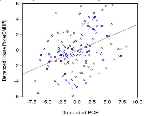
In Figure 2, I examine the direct relationship between house prices and consumption using a scatter-plot of de-trended personal consumption expenditure (PCE) and de-trended house prices (CMHPI). The data is from the Bureau of Economic Analysis (BEA) and Freddie Mac, and covers the 1970 to 2009 period. I use an HP-Filter to de-trend the data. The correlation between house prices and consumption is 0.42. As house prices increase (decrease), households are more (less) likely to consume. Given the positive correlation

3_{These observations are drawn from SIFMA data, which is available at:}

www.sif ma.org/uploadedF iles/Research/Statistics/SIF M AUSBondM arketOutstanding.pdf

between house prices and both consumption and residential investment (housing demand), housing and consumption appear to move as complements.

Figure 2: Scatterplot of Detrended CMHPI against Detrended PCE

-6 -4 -2 0 2 4 6

-7.5 -5.0 -2.5 0.0 2.5 5.0 7.5 10.0

Detrended PCE

Detrended House Price(CMHPI)

Houses are different from other durable goods in several important respects. First, changes in housing stocks incur substantial transaction costs proportional to house values. Second, the average housing depreciation rate (1.6 percent) is very small compared to the depreciation rates of other durable goods (averaging 21 percent). Third, with a required down payment, houses are highly leveraged. Fourth, house values are three times as big as all other durable good stocks. Fifth, houses perform a dual role; they are both an investment asset and a shield against fluctuations in stock prices.5 _{In the section below, I} develop a model that captures these special qualities unique to housing.

3

The Model

un-constrained households are unaffected by their collateral, provide loans to un-constrained households, receive lump sum profits from the ownership of retail firms and accumulate realtor fees. Constrained households are affected by house collateral, receive loans from unconstrained households and they are assumed to be relatively impatient in compari-son to unconstrained households. Since proportional transaction costs come from realtor fees, constrained households and entrepreneurs have to pay transaction costs to uncon-strained households (realtors), whenever there are housing transactions. Entrepreneurs produce intermediate goods using labor, houses and capital as inputs. Retailers, who buy intermediate goods from entrepreneurs and sell final consumption goods to households, are monopolistically competitive and have infrequent opportunities to adjust prices. The central bank takes the nominal interest rate as a policy instrument. Monetary policy is assumed to follow a Taylor rule responding to past inflation and past output.

The model in this paper follows the same structure as Iacoviello (2005). However, it differs in two crucial ways. First, the household utility function is not separable in housing and consumption. Introducing nonseparable preferences is a critical extension to the analysis of housing in macroeconomics. Complementarity in preferences is suggested by both micro and macro data. Second, introducing housing transaction costs leads to important changes given the nonseparable utility function. Transaction costs reduce the effect of house prices on consumption.6

In this paper, housing transaction costs proportional to the sale price of houses are introduced into the budget constraints of households and entrepreneurs. Housing transac-tion costs capture two important facts. First, new house purchases heavily depend on the sale of existing housing. These purchases are associated with realtor fees. Second, realtor fees reduce the effect of changes in house prices on consumption. As a result, transaction costs can dampen movements in house prices. In fact, introducing transaction costs moves the model closer to the data, as will be shown in section 5 and 6.

3.1 Unconstrained Households

Unconstrained households receive utility from consumption and housing services de-rived from the quantity of housing stock they hold. They also provide labor for production. Their preference for consumption and housing services is represented by a time separable

6_{Furthermore, transaction costs are important determinants of durable good consumption (Eberly}

constant elasticity of substitution (CES) utility function. Unconstrained households max-imize the following objective function:

max {b1,tC1,t,H1,t,N1,t}∞_t=0

  E0

∞

X

t=0

β₁t 1

1−ς

"

C

ε−1

ε

1,t +jt(H1,t)

ε−1

ε

ε ε−1#1−ς

−N η1 1,t

η₁

 

, (1)

where E0 denotes the expectation operator.7 C1,t denotes nondurable consumption. H1,t denotes the stock of housing.8 The discount factor β₁ for unconstrained households is assumed to be greater than that of constrained households, or 0 < β₂ < β₁ < 1. The parameterεis the elasticity of intratemporal substitution between housing and nondurable consumption. As long as ε is less than one, housing and consumption are complements. The parameterς is the curvature of the utility function, which can also be interpreted as the households’ coefficient of relative risk aversion. Households allocate their time between labor hours,N1,t and leisure,L1,t. Their endowment of time is one, henceN1,t+L1,t= 1. I also assume that the housing demand shock, jt, follows the stochastic process:

lnjt= 1−ρj

ln ¯j+ρ_jlnjt−1+εj,t, (2)

where ¯j > 0, ρ_j ∈ (−1,1) measures the persistence of the shock, and εj,t is independent and identically distributedi.i.d.∼N0;σ2_jwith mean zero and varianceσ2_j.

Each period, unconstrained households choose a level of nondurable consumption, houses and hours of work, given the period budget constraint. The budget constraint is given by

PtC1,t+ (H1t−H1t−1)Qt+Rt−1B1,t−1+ϕ1QtH1t−1=W1,tN1,t+B1,t+Ft+St.

Households begin with a stock of housing, which has the nominal market value ofH1t−1Qt. They also receive lump sum profits, Ft, from the ownership of retail firms, and nominal realtor fees, St, from constrained households and entrepreneurs. St follows

St=ϕeQtHet−1+ϕ1QtH1t−1+ϕ2QtH2t−1,

7_{Throughout the paper, the subscripts 1, 2, anderefer to unconstrained households, constrained}

house-holds, and entrepreneurs, respectively.

where ϕ₁ is zero because unconstrained households are realtors, while ϕ_e and ϕ₂ denote realtor fees, which are proportional to the sale value of houses. I assume that uncon-strained households lend in nominal terms, -B1,t. In return, they receive nominal amount of Rt−1B1,t−1. Rt−1 is the nominal interest rate. It is assumed that houses do not depre-ciate. Using a numeraire Pt, we can obtain the real budget constraint from the nominal budget constraint above:

C1,t+ (H1t−H1t−1)qt+

Rt−1

πt

b1,t−1+ϕ1qtH1t−1=w1,tN1,t+b1,t+ft+st, (3)

where w1,t is the real wage households earn from their labor supply, qt is the real house price, and πt denotes inflation, or πt = _pP_t−t₁. Since the nonseparable utility function is associated with transaction costs, the curvature, ς, can be greater than, equal to or less than the inverse of the marginal rate of intertemporal elasticity of substitution. I define the curvature of the utility function asς= _σ1.Whenεis equal toσ, the utility function becomes separable. When the limit is taken asεgoes to one, the utility function becomes the Cobb-Douglas specification. The household optimization problem is to chooseb1,t, C1,t, H1,t,and

N1,t to maximize (1), subject to constraints (2) and (3).

The first order conditions lead to the following two optimality conditions are derived:

1 =Et

_U

C1,t+1

UC1,t

β₁Rt

πt+1

, (4)

whereUC1,t=

C

ε−1

ε

1,t +jt(H1,t)

ε−1

ε

σ−ε σ(ε−1)

C

−1

ε

1,t , and

UH1,t

UC1,t

=qt(1 +ϕ1)−

πt+1

Rt

qt+1, (5)

where UH1,t =

C

ε−1

ε

1,t +jt(H1,t)

ε−1

ε

σ−ε σ(ε−1)

(H1,t)

−1

ε j

t.Equation (4) is the standard Euler equation. The intertemporal marginal rate of substitution, weighted by the nominal in-terest rate and discounted by β₁ equals one. Equation (5) determines the marginal rate of substitution between housing and consumption. These two equations can be combined into

C1

H1

= (qt)ε

(1 +ϕ₁)

jt

− πt+1

jtRt

qt+1

qt

ε

Equation (6) gives the optimal ratio of consumption to housing, which is related to house prices, transaction costs, housing demand shocks and the nominal interest rate. The higher the interest rate is, the greater consumption rises relative to housing, because houses are more sensitive to the interest rate. The higher the positive housing demand shock is, the less consumption relative to housing is likely to be, because housing is more valuable.

3.2 Constrained Households

The optimization problem for constrained households is

max {b2,tC2,t,H2,t,N2,t}∞t=0

E0 ∞

X

t=0

(β₂)t 1 1−ς

"

C

ε−1

ε

2,t +jt(H2,t)

ε−1

ε

ε ε−1#1−ς

− N η₂ 2,t

η₂ , (7)

subject to

C2,t+Ih2t+

Rt−1

πt

b2,t−1=w2,tN2,t+b2,t, (8)

where

H2t=qtH2t−1+Ih2t−ϕ2qtH2t−1

and

Rtb2t≤m2Et(qt+1πt+1H2t). (9)

For constrained households, housing transactions incur realtor fees,ϕ₂qtH2t−1. The trans-action costs are proportional to the value of house sales and are paid to unconstrained households. Since it is assumed that constrained households discount the future more heav-ily than unconstrained households, equation (9), which represents the collateral constraint, binds. As in Kiyotaki and Moore (1997), when debtors default on obligations, creditors repossess houses by paying (1−m2)βqt+1πt+1H2,t. Hence, (1−m2) can be interpreted as a down-payment ratio. The loan-to-value ratio is denoted as m2, where 0≤ m2 ≤ 1. Liquidation, however, takes times and bears costs. The collateral constraint implies that mortgages cannot exceed the house value. I assume that the housing demand shock, jt, is common to both unconstrained households and constrained households following the stochastic process.

equa-tion:

UC2,t =Rtλ

m

2,t+UC2,t+1

Rt

πt+1

β₂, (10)

qt=

UH2,t

(1 +ϕ₂)UC2,t

+β2(1−δh2) (1 +ϕ₂)

_U

C2,t+1

UC2,t

qt+1+

λm_2,t UC2,t

m2tEtqt+1πt+1

(1 +ϕ₂) , (11)

whereUC2,t =

C

ε−1

ε

2,t +jt(H2,t)

ε−1

ε

1−σε ε−1

C

−1

ε

2,t, andUH2,t=

C

ε−1

ε

2,t +jt(H2,t)

ε−1

ε

1−εσ ε−1

(H2,t)

−1

ε j_t.

λm_2,t is the Lagrange multiplier associated with the borrowing constraint. House prices de-pend onε,σ, and housing demand preferences. Composition risks, which are ratio fluctu-ations in the share of housing to consumption affect house prices. Consumption risks are also associated with house prices. The realtor fee rate,ϕ₂, affects house prices negatively. Whenε rises relative toσ, households are more willing to substitute housing services and nondurable consumption within a period than they are to substitute overall consumption between the periods. Whenεis equal toσ, house prices purely are related to composition risk and consumption risk. House prices in the steady state satisfy

q= j

(1 +ϕ₂)−β₂−(β₁−β₂)m2

C2 H2 1 ε . (12)

The house price depends on the housing demand shock, transaction costs, loan-to-values, and the ratio of consumption to house. Complementarity9,ε, is also an important element in determining asset prices. The denominator implies the average of discount factors across unconstrained households and constrained households. House prices increase when house loan-to-value m2 increases and when the realtor fee ϕ2 decreases, ceteris paribus. When the transaction costs are equal to zero, house prices are determined by the discount factor, consumption share to houses and ε. From the budget constraint, net worth is used to finance the difference of new debt and the next unit of house. Selling one’s existing house affects their net worth, which is used to purchase new stock of houses. The difference between the price of new house and net worth is the households’s new debt. Hence, houses for constrained households satisfy,

H2,t=

1

Et

qt− m2qt+1π_Rt t+1

qtH2,t−1−

Rtb2,t−1

πt

. (13)

9_{Since in this paper, the elasticity of intratemporal substitution, ε, is estimated at 0.592, it can be}

This equation is consistent with the result of Kiyotaki and Moore (1997). As the loan-to-value, m2, rises, house prices increase. This occurs because a higher loan-to-value results in higher housing demand. As house prices rise from both date t and t+ 1, the current net worth, qtH2,t−1− Rtb2_πt,t−1, and the collateral value, qt+1π_Rtt+1, increase, which induces an increase in housing demand. The extent to which houses can be used as collateral determines how much the conventional law of demand is overturned. In fact, an increase in house prices induces a rise in housing demand through the collateral effect. For the extreme case of no collateral value, or zero loan-to-value, there is a trade-off relationship between house prices and house quantity demanded. As long as the loan-to-value is positive, house prices are positively related to house quantity demanded.

Equation (13) implies the transmission mechanism of house prices to macroeconomic fluctuations. Suppose house prices rise. Overall, a rise in house prices increases borrowing capacity and net worth. Housing and consumption are boosted because of heightened collateral values and net worth. In turn, higher housing demand further increases house prices. The change in housing net worth is associated with a high leverage effect, measured in the loan-to-value, which makes net worth much higher relative to a required down payment. Indeed, leverage plays an amplifying role in net worth.10 _{The converse holds} when there is a decline in house prices. As the leverage ratio rises, it decreases net worth. Households may default due to negative equity. Housing and consumption can shrink because of tighter borrowing constraints, as a fall in collateral values, and net worth, further depresses housing and consumption. Therefore, changes in house prices amplify fluctuations in macroeconomic variables.

3.3 Entrepreneurs

The Entrepreneurs derive utility only from consumption. They produce intermediate goods according to the following constant return to scale (CRS) Cobb-Douglas production function with labor, housing and capital as inputs, which can be written as

Yt=Zt Ktv−1Ht1−−1v

µ

N_1,tαN_2,t(1−α)(1−µ), (14)

10_{“The usual notion that a higher land price,q}

t, reduces the farmers demand is more than offset by the

facts that (i) they can borrow more whenqt+ 1 is higher, and (ii) their net worth increases asqt rises”

whereYtdenotes output andZtrepresents productivity in period t. Kt−1andHt−1 denote capital and housing in period t-1, respectively. Furthermore, Kt−1 and Ht−1 are initial endowments to entrepreneurs. The shock toZt follows the stochastic process:

lnZt= (1−ρz) ln ¯Z+ρzlnZt−1+εZ,t, (15)

where ¯Z >0,ρ_Z ∈(−1,1) measures the persistence of the shock and εZ,t is a white noise process with mean zero and varianceσ2_Z. Capital accumulation follows

Kt= (1−δKe)Kt−1+IKt−

ξ

2

(Kt−Kt−1)2

Kt−1

,

where Ikt denotes investment of capital. The parameter ξ denotes convex adjustment parameter. Capital depreciates at the rateδKe. Housing accumulation follows

Het =qtHet−1+IHet−ϕeqtHet−1,

where IHet denotes investment of houses. Housing transactions are associated with the transaction costs like realtor fees,ϕ_eqtHet−1, which are paid to unconstrained households. The utility function, budget constraint and borrowing constraint of entrepreneurs can be represented by the utility maximization problem as follows:

max

{Cet,bet,It,Kt,Ht,N1,t,N2,t}∞_t=0

E0 ∞

X

t=0

γtlnCet, (16)

subject to

Yt

Xt

+bet =Cet+Rt−1

πt

bet−1+w1,tN1,t+w2,tN2,t+Ikt+IHet+ξKt+ξHet, (17)

where

IKt=Kt−(1−δ)Kt−1 , ξKt = ψK

2δ

IKt

Kt−1 −δ

2

Kt−1, IHet={Het−Het−1}qt,

ξ_Het=ϕ_eqtHet−1,

and

There is a proportional housing transaction costs parameter,ϕ_e, in the budget constraint. Finally, me is the constant parameter of the loan to value ratio to entrepreneurs.

3.4 Retailers

Retailers as in Iacoviello (2005), which follows Bernanke, Gertler and Gilchrist (1999) take the same firms. Retailers produce a continuum of differentiated final goods modeled under monopolistic competition. Since retailers have market power, profits are assumed to be paid to unconstrained households. The retailers’ supply curve implies a Phillips curve, determined by an optimal pricing equation. Retail prices are sticky, and the probability of any retailers being able to adjust its nominal prices is 1−θ. The retailers purchase intermediate goods from entrepreneurs with the price of P_tinter and sell final goods to households with the price,Pg, where the goods are differentiated on a unit interval. Final

goods are Yt(G) =

_R1

0

Yt(g)(ξ−1)/ξdg

ξ ξ−1

with ξ > 1. The solution to the firms’ cost

minimization problem gives a demand function for intermediate goods and a price index,

Pt = R₀1Ptinter(g)1−ξdg

1 1−ξ

. Profit maximization by each retail firm implies that the

optimal price of final goods,P⌢t(g), satisfies ∞

P

i=0

θiEt

β C1,t

C1,t+i

⌢

Pt(g)

Pt+i −

Xt

Xt+i

⌢

Yt+i(g)

= 0,

where Xt is the markup. The aggregate price index is Pt =

θP_tε₋₁+ (1−θ)P⌢1_t−ξ

1 1−ξ

.

From the optimization of retailers, the aggregate supply curve can be derived as ˆπt =

βπˆt+1−kXˆt+ ˆεu,t, wherek= (1−θ)(1_θ−βθ).

3.5 The Central Bank

The central bank is assumed to follow a Taylor Rule taking the nominal interest rate as the instrument for monetary policy:

Rt= (Rt−1)γR

π1+γπ

t−1

Yt−1

Yt

γy

qγq

t−1

1−γR

εR,t (19)

3.6 Equilibrium

borrowing constraints and first order conditions for each economy. For the markets to clear, the bond market forbt, goods market forYt and the house market forHet, H1t and H2t should meet the following conditions:

(a)N1t=N2t

(b)He,t+H1,t+H2,t= 1, (c)Ce,t+C1,t+C2,t+It=Yt, (d)It=IKt+IHet+IH1t+IH2t,

(e)st=ϕeqtHet−1+ϕ1qtH1t−1+ϕ2qtH2t−1, (f)bt+b1t+b2t= 0

Wages are different across households and based on their productivity. In the steady state, unconstrained households receive wage bills ofw1N1 =α(1−µ−v)Y, while constrained households receive a wage bill ofw2N2 = (1−α)) (1−µ−v)Y. 11

3.7 Solution Method

The solution of the dynamic model involves non-linear equations and identity equations. The steady state values of the state variables are recovered from a nonlinear system of equations. This step uses the Broyden method for solving systems of nonlinear equations. After obtaining steady state values, the model is loglinearized. All derivatives of the first order conditions are automatically calculated using the Jacobian command in Matlab. Finally, the Uhlig toolkit is used to solve the linear system of stochastic difference equations.

4

Calibration and Estimation

4.1 Calibration

The steady state value for labor hours for both unconstrained households and con-strained households is 0.33. The housing preference parameter,j, is set to 0.21 in order to match the share of GDP. Following Luengo-Prado and Sorensen (2006), and Li, Liu and Yao (2008), and Stokey (2007), the transaction costs for constrained households is 5 percent. This is consistent with the data from the Department of Justice in 2009. The benchmark model assumes a lower level of 3 percent as the transaction cost of entrepreneurs. In the

sensitivity analysis, 6 percent for entrepreneurs is also applied. Either 3 percent or 6 per-cent can be applied without changing results. Also recall that unconstrained households, as realtors, pay no transaction costs.

The discount factors for unconstrained households, constrained households and en-trepreneurs, the share of housing to consumption, the parameters of production across capital and housing, the probability of the price adjustment and the depreciation rate for housing are the same values as in Iacoviello (2005).

Table 1: Calibration

Parameter Value Data to Match

β ,γ,β₂ 0.99, 0.98, 0.97 subjective discount rate

j 0.21 share of housing to consumption

ϕ₁,ϕ_e,ϕ₂ 0.0, 0.03, 0.05 housing transaction costs

η 1.01 elasticity of labor

δ 0 depreciation of housing

µ,ν 0.3, 0.03 share of capital and housing

X 1.05 markup

θ 0.75 probability of the fixed price

4.2 Estimation

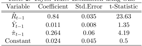
4.2.1 Monetary Policy

For monetary policy, I assume that the nominal interest rate responds to past inflation and past output through the following Taylor Rule, which is a log-linearization of Equation (19):

ˆ

Rt=αRRˆt−1+ (1−αR)

(1 +απ) ˆπt−1+αYYˆt−1

+ ˆεR,t. (20)

I estimate the parameters of the Taylor Rule using the OLS method.

Table 2: Taylor Rule: Estimation using OLS Variable Coefficient Std.Error t-Statistic

ˆ

Rt−1 0.84 0.035 23.63

ˆ

Yt−1 0.011 0.008 1.35

ˆ

πt−1 0.264 0.06 4.19

Monetary policy makers respond to past inflation and output through a lagged interest rate. The coefficients are estimated: Rbt = 0.84

(0.03)Rbt−1 + 0(0.06).26πbt−1+ 0(0.008).011ybt−1.

12 _Hence

Equation (20) can be written as

b

Rt= 0.84

(0.03)Rbt−1+ 0.16

1.5

(0.06)bπt−1+ 0(0.008).069ybt−1

. (21)

4.2.2 Estimation

The crucial parameter for the model is the elasticity of substitution of housing for consumption. Here, I discuss two estimates of this parameter. The first involves a co-integration method. The second uses minimum distance estimation between model and data impulse responses.

Using NIPA data, I estimate this elasticity of intratemporal substitution, ε, to be 0.19 (Song (2009)) using a co-integrating method. I find a significant estimate of this elasticity of substitution, ε, to be 0.19. The key point for this significance is the time period of the data. The sample period is important because different sample periods provide dif-ferent significance of statistical analysis. The sample period of NIPA data is from 1970 through 2009, which is different from the samples from 1947 to 2001 as in Piazzesiet al.

(2007). The relative price is the ratio of the price index of housing services to the price index of nondurable consumption. I use co-integration approach to parameter estimation. The complementarity, or the elasticity of intratemporal substitution between housing and consumption is estimated at 0.19, 0.19 and 0.18 through DOLS, CCR and FMOLS, respec-tively. Piazzesiet al. (2005) also use NIPA data to estimate the parameter of the elasticity of substitution using co-integration method, which, however, is not significant statistically. The data in their paper is used in two different categories: long sample periods (1936-2001) and post-war sample periods (1947-(1936-2001). The results are different based on the the beginning period of 1936 and 1947. However, the periods from 1970 through 2009 as in Song (2009) significantly provide co-integration trends. This finding is consistent with the results of Flavin and Nakagawa (2004) who apply GMM to the PSID. They estimate the EIS at 0.13.

For robustness, instead of using co-integrating method through which I identified com-plementarity, I broadly follow the methodology of Iacoviello (2005) in that I use minimum

12_{Following Equation (2), the coefficients are transformed into (1−α}

R) (1 +απ) = 0.26→α_π= 0.26 (1−αR)

−

distance estimation using macro data from 1970:Q1 to 2008:Q4, such as the Federal Fund Rate (fedfunds), inflation ( GDP deflator), house prices (CMHPI), and real GDP (GDPC1). However, this estimation still differs from Iacoviello (2005) in substantive ways. First, I use a different time period. Second, I add two more structural parameters: 1) the elasticity of intratemporal substitution,ε, and 2) risk aversion,ς.

The EIS, ε, is estimated at 0.592 with a standard error of 0.053, thus providing strong support of preferences over housing and consumption for nonseparability and complemen-tarity. I estimate the empirical impulse responses using the VAR method. The Choleski ordering is the Fed Fund Rate, inflation, house prices and the output gap. The distance function is f(b) = IRFM(b)−IRFD, where IRFM(b) is the impulse responses obtained from the model, IRFD is the data responses from the VAR, and b is the vector of pa-rameters (ε, σ, σu, σj, σa, ru, rj, ra, a, m1, m2). There exist solutions to the minimization of

Jt(b) = M IN b

"

f

(314×1)

(b)T Φ

(314×314)(314f×1) (b)

#

,where Φ = W

314×314 Ω −1

314×314, where Ω

−1 _{is the}

inverse matrix of the sample variance of the IRFs.

Table 3: Estimation

Parameter Value STD.e Parameter Value STD.e

ε=elasticity of substitution 0.592 0.053 φ_π =autoregressiveπ 0.629 0.043

ς =curvature 2.317 0.357 φ_=autoregressivej 0.885 0.017

a=share of wage 0.553 0.046 φ_a=autoregressivea 0.177 0.1

me=loan−to−valuee 0.412 0.066 σA=stdeva 9.195 3.5

m2 =loan−to−value2 0.861 0.02 σj =stdevj 0.021 1.64

σR=stdevR 0.24 0.009 σπ =stdevπ 0.154 0.024

5

Results

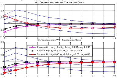
5.1 The Issue of Separable Preferences with housing transaction costs

Panel (B) introduces transaction costs. The triangled, squared, and circled lines are the impulse responses of aggregate consumption to the increase in house prices. The house loan-to-value ratios of those three lines for entrepreneurs and constrained households are set to (0.1 percent, 0.1 percent), (45 percent, 30 percent) and (89 percent, and 55 percent), respectively.

Figure 3: Separability and Proportional Transaction Costs

0 1 2 3 4 5 6 7 8 9 10

-0.4 -0.2 0 0.2 0.4

0.6 (A). Consumption WIithout Transaction Costs

0.24

0 1 2 3 4 5 6 7 8 9 10

-0.4 -0.2 0 0.2 0.4

0.6 (B). Consumption With Transaction Costs

-0.26 -0.17 -0.26 -0.17 -0.26 -0.17 -0.36 -0.17

Separability, adj_e=0, adj₂=0, m_e=0.001, m₂=0.001 Separability, _e=0, ₂=0, m_e=0.45, m₂=0.3 Separability, _e=0.03, ₂=0.05, m_e=0.89, m₂=0.55

Panel (A) is a replication of Iacoviello (2005) with his log utility function. As in his paper, there are no housing transaction costs. With loan-to-value ratios of 89 percent for entrepreneurs and 55 percent of constrained households, aggregate consumption rises by 0.24 percent after an 1 percent increase in house prices. In this consumption response, the loan-to-value ratios are critical factors, which make the model successful, so that the response matches the data within the 90 percent confidence intervals. The other loan-to-value ratios do not induce effective co-movement between housing and consumption. Hence, the co-movement between house prices and consumption depends on the loan-to-value ratio.

con-sumption, I compare the circled line in Panel (A) with that in Panel (B). The circled line in Panel (B) shows the consumption response with the presence of transaction costs of 5 percent and 3 percent for constrained households and entrepreneurs respectively.13

Critically, once we introduce empirically plausible levels of transaction costs, the posi-tive consumption response to a rise in house prices disappears. Transaction costs dominate and dampen the effects of loan-to-value ratios so that aggregate consumption no longer increases following a rise in house prices. The aggregate consumption response is severely affected by transaction costs. In other words, housing transaction costs nullify the effect of loan-to-value ratios on consumption. Hence, separable utility function between housing and consumption in this model, cannot generate a co-movement between house prices and consumption when housing transactions costs are introduced.14

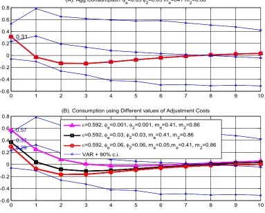
5.2 Complementarity between Housing and Consumption

Figure 4 resolves the problem caused by housing transaction costs in Figure 3. The so-lution relies on the introduction of nonseparable preferences over housing and consumption. Since the extent of non-separability of preferences is jointly determined by the elasticity of intratemporal substitution,ε, and curvature,ς, the parameters are now jointly estimated. The estimates of ε and ς are 0.59 and 2.3, respectively. As before, a rise in house prices is generated by a shock to housing demand, j, common across households. The house loan-to-value ratios, for entrepreneurs and constrained households, are set to 41 percent and 86 percent, respectively.

Panel (A) shows that complementarity induces a positive aggregate consumption re-sponse following a positive house price shock of 1 percent. When housing transaction costs are set to 5 percent and 3 percent for constrained households and entrepreneurs, respec-tively, the consumption response rises to 0.31 percent, which falls within the 90 percent confidence intervals of the data.

Panel (B) examines the sensitivity of my results with respect to housing transaction costs, fixing the loan-to-value ratios for entrepreneurs and constrained households to 41

13_{In the sensitivity, 6 percent is applied.}

14_{Empirical impulse responses come from the estimated VAR using the data of federal fund rate, real}

percent and 86 percent, respectively.

Figure 4: Complementarity with Transaction Costs and Loan-to-Values

0 1 2 3 4 5 6 7 8 9 10

-0.6 -0.4 -0.2 0 0.2 0.4 0.6 0.8

(A). Agg.Consumption: _e=0.03 ₂=0.05 m_e=041 m₂=0.86

0.31

0 1 2 3 4 5 6 7 8 9 10

-0.6 -0.4 -0.2 0 0.2 0.4 0.6

0.8 (B). Consumption using Different values of Adjustment Costs

0.57 0.37 0.29

=0.592, _e=0.001, ₂=0.001, m_e=0.41, m₂=0.86

=0.592, _e=0.03, ₂=0.03, m_e=0.41, m₂=0.86

=0.592, _e=0.06, ₂=0.06, m_e=0.05,m_e=0.41, m₂=0.86 VAR + 90% c.i.

As transaction costs increase to 6 percent for all agents, the aggregate consumption response at the impact date falls to 0.29 percent. Consumption soars when transaction costs are close to zero with the consumption response climbing to 0.57 percent, which causes the response to lie outside the 90 percent confidence intervals. In other words, when there are no transaction costs, the consumption response becomes implausibly large.15

15_{The confidence intervals come from the VAR, estimated from the data for federal fund rate, inflation,}

5.3 Consumption Across Households

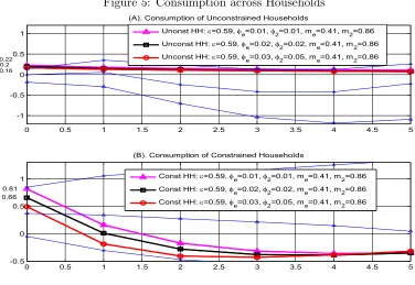
In Figure 5 I investigate how an 1 percent increase in house prices affects consump-tion of different households as transacconsump-tion costs vary. There are two types of households: constrained and unconstrained. Aggregate consumption data on these types of households are taken from Consumer Expenditure Surveys from 1984:Q1 to 2008:Q4. Constrained households are assumed to be young households (below 35 years old) whose housing pur-chase is typically highly leveraged, as in Flavin and Yamashita (2002). On the other hand, unconstrained households are assumed to be relatively old households (over 35 years old). The model’s parameters for complementarity and loan to value ratios for entrepreneurs and constrained households are set to 0.59, 0.41 and 0.86, respectively.

Figure 5: Consumption across Households

0 0.5 1 1.5 2 2.5 3 3.5 4 4.5 5

-1 -0.5 0 0.5 1

(A). Consumption of Unconstrained Households

0.160.2 0.22

0 0.5 1 1.5 2 2.5 3 3.5 4 4.5 5

-0.5 0 0.5 1

(B). Consumption of Constrained Households

0.81 0.66

Unonst HH: =0.59, _e=0.01, ₂=0.01, m_e=0.41, m₂=0.86 Unconst HH: =0.59, 

e=0.02, 2=0.02, me=0.41, m2=0.86 Unconst HH: =0.59, _e=0.03, ₂=0.05, m_e=0.41, m₂=0.86

Const HH: =0.59, _e=0.01, ₂=0.01, m_e=0.41, m₂=0.86 Const HH: =0.59, 

e=0.02, 2=0.02, me=0.41, m2=0.86 Const HH: =0.59, _e=0.03, ₂=0.05, m_e=0.41, m₂=0.86

prices than unconstrained households.

Panel (A) shows the consumption response of unconstrained households. Initially, un-constrained households increase consumption by around 0.2 percent. Moreover, the slope of their consumption response is generally flat. Interestingly, their consumption response does negligibly vary when facing different transaction costs. Therefore, transaction costs do not significantly affect the consumption responses of unconstrained households. The consumption response for constrained households is illustrated in Panel (B). Overall, con-strained households are substantially more responsive to the increase in house prices than unconstrained households. In fact, as transaction costs decrease, the consumption response rises to 0.5 percent, 0.66 percent and 0.81 percent. Contrary to unconstrained households, transaction costs are a significant factor for credit-constrained households.

The implication is as follows. Suppose there is a rise in house prices. The marginal propensity of consumption (MPC) out of gains in house prices for constrained households is larger than that for unconstrained households. This difference in the MPC across house-holds leads to a change in overall aggregate consumption. Constrained househouse-holds are likely to use their increase in housing collateral value to finance an increase in consumption that exceeds the house price increase.

5.4 The Effect of Elasticity of Intertemporal substitution on Consump-tion across Households

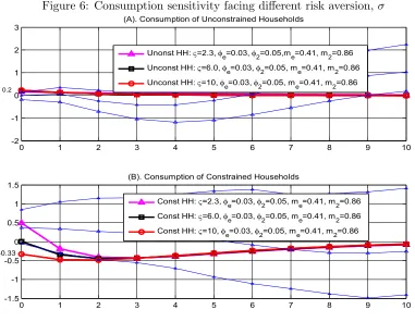
Figure 6 illustrates how an 1 percent increase in house prices affect consumption across heterogeneous households with respect to the elasticity of intertemporal substitution,

σ = 1/ς. The consumption response to an 1 percent increase in house prices is displayed with respect to ς. Transaction costs and loan-to-values for entrepreneurs and constrained households are set to 3 percent, 5 percent, 41 percent and 86 percent, respectively. I applied the parameter values of 2.3, 6 and 10 forς in order to consider the case when risk aversion is normal, high and very high for unconstrained households (Panel A) and for constrained households (Panel B). The EIS is held fixed at 0.59.

Panel (A) displays the effect of risk aversion on consumption of unconstrained house-holds. The consumption responses facing different values of risk aversion are negligibly different. Risk aversion does not significantly affect the consumption decision for uncon-strained households.

Figure 6: Consumption sensitivity facing different risk aversion,σ

0 1 2 3 4 5 6 7 8 9 10

-2 -1 0 1 2

3 (A). Consumption of Unconstrained Households

0.2

0 1 2 3 4 5 6 7 8 9 10

-1.5 -1 -0.5 0 0.5 1

1.5 (B). Consumption of Constrained Households

-0.33

Unonst HH: =2.3, _e=0.03, ₂=0.05,m_e=0.41, m₂=0.86 Unconst HH: =6.0, _e=0.03, ₂=0.05, m_e=0.41, m₂=0.86 Unconst HH: =10, _e=0.03, ₂=0.05, m_e=0.41, m₂=0.86

Const HH: =2.3, _e=0.03, ₂=0.05, m_e=0.41, m₂=0.86 Const HH: =6.0, _e=0.03, ₂=0.05, m_e=0.41, m₂=0.86 Const HH: =10, _e=0.03, ₂=0.05, m_e=0.41, m₂=0.86

Generally, higher risk aversion induces lower initial consumption. Whenς = 10, the initial rise in the consumption of constrained households seen at lower levels of risk aversion is completely overturned. When risk aversion is 2.3, the consumption response to an 1 percent rise in house prices is 0.5 percent.

Overall, risk aversion affects consumption decisions of constrained households. Even a positive house price shock can lead to a fall in consumption when risk aversion is high, that is when households are unwilling to substitute consumption inter-temporally. The effect of a low elasticity of intertemproal substitution offsets the positive effect of house prices.

6

Results for Monetary Policy

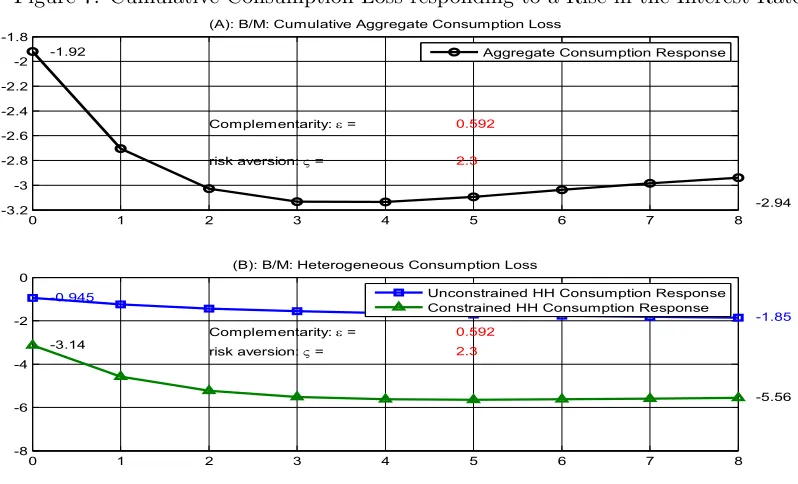
housing and consumption, affects the effective degree of risk aversion across households. This leads to different consumption responses in response to an increase in interest rates. Figure 7 shows a cumulative consumption loss across households after an 1 percent in-crease in interest rates for benchmark. Panel (A) is the aggregate cumulative consumption response to tighter monetary policy. Aggregate consumption falls to 1.92 percent initially. Panel (B) shows that an increase in interest rates decreases consumption for both con-strained and unconcon-strained households. However, this decrease is larger for concon-strained households.

Figure 7: Cumulative Consumption Loss responding to a Rise in the Interest Rate

0 1 2 3 4 5 6 7 8

-3.2 -3 -2.8 -2.6 -2.4 -2.2 -2 -1.8

-2.94 -1.92

(A): B/M: Cumulative Aggregate Consumption Loss

Complementarity:  = 0.592

risk aversion:  = 2.3

Aggregate Consumption Response

0 1 2 3 4 5 6 7 8

-8 -6 -4 -2 0

-1.85

-5.56

-0.945

-3.14

(B): B/M: Heterogeneous Consumption Loss

Complementarity:  = 0.592

risk aversion:  = 2.3

Unconstrained HH Consumption Response Constrained HH Consumption Response

stronger complementarity effect on consumption of unconstrained households is different from that of constrained households. Unconstrained households are not significantly sensi-tive to an increase in interest rates because they are not constrained by housing collateral, and they can initially benefit from more interest amount as lenders. Stronger comple-mentarity magnifies the effect of interest rates, so that the gap between two consumption responses across heterogeneous households widens.

Figure 8: Cumulative Consumption Loss responding to a Rise in the Interest Rate

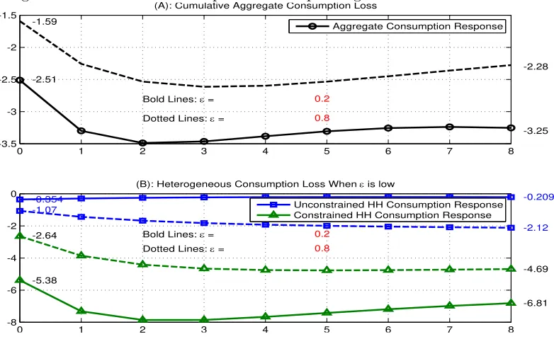
0 1 2 3 4 5 6 7 8

-3.5 -3 -2.5 -2 -1.5

-3.25 -2.51

(A): Cumulative Aggregate Consumption Loss

Bold Lines:  = 0.2

-2.28 -1.59

Dotted Lines:  = 0.8

0 1 2 3 4 5 6 7 8

-8 -6 -4 -2

0 _-0.209

-6.81 -0.354

-5.38

(B): Heterogeneous Consumption Loss When  is low

Bold Lines:  = 0.2 -2.12

-4.69 -1.07

-2.64

Dotted Lines:  = 0.8

Unconstrained HH Consumption Response Constrained HH Consumption Response

Aggregate Consumption Response

In Figure 8, the dotted lines show the case in which the degree of complementarity,

omy to monetary policy. Figure 9 shows the effects of annual one percent increase in the interest rate on aggregate consumption. Panel (A) and Panel (B) are the benchmark based on the estimated or calibrated parameter values: curvature,ς, and complementarity,

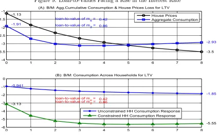
ε, are set to 2.3 and 0.592, respectively. Loan-to-values for entrepreneurs and constrained households are set to 42 percent and 86 percent, respectively. As already seen, a rise in the interest rate serves to significantly decrease house prices and consumption as shown in Panel (A) and Panel (B). The decrease in consumption is larger for constrained households.

Figure 9: Loan-to-Values Facing a Rise in the Interest Rate

0 1 2 3 4 5 6 7 8

-4 -3.5 -3 -2.5 -2 -1.5 -1

-3.5 -2.93 -1.13

-1.91

(A): B/M: Agg.Cumulative Consumption & House Prices Loss for LTV

loan-to-value of m_e = 0.42 loan-to-value of m₂ = 0.86

House Prices

Aggregate Consumption

0 1 2 3 4 5 6 7 8

-6 -5 -4 -3 -2 -1 0

-1.85

-5.55 -0.941

-3.13

(B): B/M: Consumption Across Households for LTV

loan-to-value of m_e = 0.42 loan-to-value of m₂ = 0.86

Unconstrained HH Consumption Response Constrained HH Consumption Response

consumption losses across constrained households and unconstrained households is 4.59 percent and 1.02 percent, respectively. This cumulative loss of consumption to an increase in interest rates is significantly larger for constrained households, and the gap between the two impulse responses widens as loan-to-value ratios increase.

Figure 10: Loan-to-Values Facing a Rise in the Interest Rate

0 1 2 3 4 5 6 7 8

-5 -4 -3 -2 -1

-4.59 -3.77 -1.31

-2.74

(A): B/M: Agg.Cumulative Consumption & House Prices Loss for LTV

loan-to-value of m_e = 0.8 loan-to-value of m₂ = 0.91

House Prices

Aggregate Consumption

0 1 2 3 4 5 6 7 8

-7 -6 -5 -4 -3 -2 -1

-2.24

-6.48 -1.02

-4.59

(B): B/M: Consumption Across Households for LTV

loan-to-value of m_e = 0.8 loan-to-value of m₂ = 0.91

Unconstrained HH Consumption Response Constrained HH Consumption Response

7

Conclusion

between housing and consumption.

My model generates differing elasticities of response across households following aggre-gate shocks. Following changes in both house prices and interest rates, the consumption response of credit-constrained households is greater than that of unconstrained households. I trace this differing responsiveness in consumption to the house loan-to-value ratios char-acterizing credit-constrained households. Loan-to-value ratios amplify the effect of changes in interest rates on consumption especially for credit-constrained households. I also find that the differences widen with the degree of complementarity between housing and con-sumption.

Following a rise in house prices, the net worth of credit-constrained households in-creases, which boosts their access to credit. This, in turn, allows constrained households to raise their spending on consumption and housing. Moreover the resulting rise in hous-ing demand leads to a further increase in house prices. While transaction costs abate this process somewhat, the fundamental co-movement between housing and consumption persists.

REFERENCES

[1] Aoki, Kosuke;Proudman, James and Vlieghe Gertjan,“House prices, Consumption, and Monetary Policy: a Financial Accelerator Approach”,Journal of Financial Intermediation, 2004, 13, pp. 414-35.

[2] Bernanke, Ben S. and Gertler, Mark. “Inside the Black Box: Credit Channel of Mone-tary Policy Transmission”,Journal of Economic Perspectives, Fall 1995, 9 (4), pp. 27-48. [3] Campbell, John Y. and Cocco, Joao F., “How do house prices affect consumption? Evidence from micro data”, Journal of Monetary Economics, 2006,

[4] Christiano, Lawrence J., Eichenbaum, Martin and Charles Evans, “Nominal Rigidities and the Dynamic Effects of a Shock to Monetary Policy”, Journal of Political Economy, 2005, 113(1), pp. 1-46.

[5] Robert B. Couch, “Portfolio Choice with complementarity housing”, Working Paper, 2004.

[6] Eberly, Janice C., ”Adjustment of Consumers’ Durables stocks: Evidence from Autom-bile Purchases”,Journal of Political Economy, June 1994, pp. 403-436.

[7] Iacoviello, Matteo;“House Prices, Borrowing Constraints and Monetary Policy in the Business Cycle”,American Economic Review, June 2005, 95 (3), pp. 739-764.

[8] Flavin,Marjorie and Nakagawa Shinobu;“A Model of Housing in the Presence of Ad-justment costs: A structural interpretation of habit persistnce”,NBER, April 2004. [9] Flavin,Marjorie and Yamashita Takashi;“Owner Occupied Housing and the Composi-tion of the Household Portfolio”,American Economic Review, December 2002.

[10] Grossman,Sanford J. and Laroque, Guy.;“Asset Pricing and Opitmal Protfolio Choice in the Presence of Illiquid Durable Consumption”,Econometrica, January 1990, 58(1),pp.25-51.

[11] Hanushek, Eric A. and John M. Quigley.;“What is the price elasticity of housing de-mand?”, Review of Economics and Statistics, 1980, 62,pp.449-454.

[12] Kato,Ryo;“A User Guide for Matlab Code for an RBC Model Solution and Simula-tion”,FRB of Philadelphia Working paper , March 2009: No. 09-7.

[13] Kiyotaki,Nobuhiro and Moore,J;“Credit Cycles”,Journal of Political Economy, 1997: Vol.105 pp.211-248.

Structural Estimation”, Working paper, ISBN: 0-262-13420-9.

[16] Luengo-Prado,Maria Jose, and Sorensen,Bent E. “Measuring intertemporal substitu-tion: the role of durable goods”. Journal The Review of Economics and Statistics, 2008, Vol 90, 65-80.

[17] Miranda,Mario and Fackler, Paul;“Applied Computational Economics and Financeo”,

MIP Press, ISBN: 0-262-13420-9.

[18] Ogaki, Massao, and Reinhart. “What Can Explain Excess Smoothness and Sensitivity of State-Level Consumption?”. Journal of Political Economy, 1998, 1078-1098.

[19] Piazzesi, Monika, and Schneider, Martin. “Inflation and the Price of Real Assets”.University of Chicago, mimeo, 2006.

[20] Piazzesi, Monika, Schneider, Martin, and Sleale Tuzel. ”Housing, consumption and asset pricing”,Journal of Financial Economics, 83 (2007) 531-569.

[21] Siegel, Stephan ”Consumption-based asset pricing: durable goods, adjustment costs, and aggregation”,Working Paper, Columbia University (2004).

[22] Song,Inho. ”Complementarity in Housing and Monetary Policy”, Working Paper, (2009).