http://dx.doi.org/10.4236/jamp.2016.46118
A Method for the Solution of Educational
Investment
Jun’e Liu
1, Le Yu
2, Xiaolin Liu
21The School of Information, Beijing Wuzi University, Beijing, China 2Graduate Department, Beijing Wuzi University, Beijing, China
Received 17 May 2016; accepted 26 June 2016; published 29 June 2016
Copyright © 2016 by authors and Scientific Research Publishing Inc.
This work is licensed under the Creative Commons Attribution International License (CC BY). http://creativecommons.org/licenses/by/4.0/
Abstract
In order to improve the performance of higher education in the United States, the Goodgrant Foundation intends to donate a total of $100,000,000 (US 100 million) to an appropriate group of schools per year, for five years, starting in July 2016. For this, our team puts forward upon an op-timal investment strategy, which includes the schools to invest, the investment amount of each school, and the return due to investment, to solve this problem. Our main idea is as follows. First of all, we choose suitable investment school universities in the United States. Secondly, we use Analytic Hierarchy Process to get the rate of return on investment and venture capital. Thirdly, we establish a venture capital return model. Finally, solving the mathematical model ensures the in-vestment amount of each school and the return due to inin-vestment. To implement this strategy, first of all, we obtain the candidate school based on students score card. Then, according to the factor analysis, we analyze the factors which mainly affect the choice of school. Secondly, we em-ploy Analytic Hierarchy Process to get the rate of return on investment and capital risk. In the end, we establish a risk return model to get investment amount for each school, amount of risk and re-turn. In order to ensure the minimum risk and the maximum return, we set up a multi objective programming model and solve it by using the constraint method. We get the result that includes the maximum net profit of the investment and risk loss rate. According to statistical analysis, we can get the overall return of net income within five years. Finally, we choose 320 candidate schools and get the investment amount of each school according to the principle of as many schools as possible. We have proved that the foundation will receive a return of more than 295.363 million in the next 5 years. After-verification, our strategy can be directly applied to the investment field and get good results.
Keywords
1. Introduction
In the era of knowledge economy, higher education, as a social intelligence incubator, is more and more impor-tant. Every country develops vigorously its higher education to improve their comprehensive strength and com-petitiveness. Well higher education’s development must have education funds, but the education funds from government drop year by year, and the shortage of education funds has restricted the development of higher education. Therefore, colleges and universities should actively raise funds from the society, use and manage the funds for better development.
The Goodgrant Foundation is a charitable organization that wants to help improve educational performance of undergraduates attending colleges and universities in the United States. It has a important goal that millions of students can get the best education resources across the country. The special fund can help build a bridge for the development of education, especially schools and students in poor areas. At the same time, it also helps the children who have dropped out of school in the poor families and develops more aid activities. Starting in July 2016, the foundation intends to donate a total of $100,000,000 (US 100 million) to an appropriate group of schools per year, for five years.
To provide high quality foundation with an optimal investment decisions, we are using the Analytic Hierarchy Process (AHP) to given weights for many factors influencing the investment returns under the predecessors’ re-search. To establish the risk investment model, through the constraint method, we transform the multi-objective model to a single objective model.
2. Problem Analysis
By analyzing the data and casual working, we can get basic information about 2977 American universities, which include school location, size and nature, degree-granting conditions, undergraduate education enrollment, the students’ proportion of each race, student retention and completion rates, students’ race, family income situ-ations, important subjects scores in school, the cases of scholarships and loan accepted, the average debt, re-payment ability, the income after works and so on. In the big background of American education, we fully ana-lyze the obtained data and establish a suitable model to help Goodgrant Foundation decide an optimal quality investment strategy, which include the school to invest, the money of investment in each school, the investment of time, and repay of investment returns.
3. Analysis Process
First of all, we analyze existing data. We selected 2936 schools from 7804 schools of most recent cohort data and analyze these date to find out the bigger influencing factors. Then by considering some factors, we deter-mine 583 schools of investment in program ways. But in these 583 schools we selected, there are many null date in some schools. In order to avoid risks and reduce the risk of investment, we removed the more uncertainty schools. The end result that we choose is investment of schools.
Secondly, Considering Various factors of effecting return on investment, Determining influence level of these factors, selecting three greatest impact factors and applying for Analytic Hierarchy Process to determine repay of invest. Similarly, using the same method gets risk-free rate.
Next, according to the principle of minimum investment risk and maximum return on investment, Building risk investment return model by assigning to each school investment and total investment constraints.
Besides, by solving the risk return on investment model, obtaining the money of investment in each school and obtain repay on investment within a year. Suppose the return on investment every year is the same in five years, and then get to the expected return within five years.
In the end, Analysis of the results obtained, Evaluation of the model, the model summary and summary of outcome to analysis strength and weakness of model and give Valuable comments and suggestions.
4. Basic Assumptions
We make the following assumptions about all the process of solve the problem in this paper.
1) The influence of professional may be ignored, we only consider the investment of every school. 2) Every school of investment and return for every year are assumed to be the same.
Additional assumptions are made to simplify analysis for individual sections. These assumptions will be dis-cussed at the appropriate locations.
After the text edit has been completed, the paper is ready for the template. Duplicate the template file by using the Save As command, and use the naming convention prescribed by your journal for the name of your paper. In this newly created file, highlight all of the contents and import your prepared text file. You are now ready to style your paper.
5. Model Development
5.1. The Data Processing
Before presenting our models, we describe the preprocessing work that we did with the data. 5.1.1. Screen out the Date of Investment School
1) Comparing the name of institution in Most Recent Cohorts Date (Scorecard Elements), than selecting out 2936 institutions from the currently certified in operating by the C Programming Language.
2) Using factor analysis compare the different criterion to influence The Goodgrant Foundation’s choice of investment of institution by some subjective cognition, and using Statistical Product and Service Solutions to select some institutions from the step 1 through some much important criterion including HCM2, PREDDEG, CONTROL, LOCALE etc. As followers, Figure 1 stands for the correlation of three variables.
Analyzing factors that influence the choice of investing school for the following reasons:
a) HCM2 indicates the school has special scholarship, which proves that the floating capital of the school is more. Hence, these schools don’t need too much investment and this factor has greater impact on school choice.
b) PREDDEG indicates the situations of degree classification. If schools have more classification situations, the teachers of school are much stronger. We can’t invest the school, so this factor has greater impact on school choice.
c) CONTROL indicates the nature of school, which is public school, private school, for-profit or non-profit. If the school is a public school, the government will invest much funding. If the school is a private for-profit school, it has additional income, so we would give more consideration to non-profit school. Therefore these factors have greater impact on school choice.
d) LOCALE indicates the size of city, if the school is located in the large scale city, which representative the cost of education is more. So we should give more investment. Therefore, this factor has much greater impact on school choice.
There are 18 factors like these above. We don’t list one by one. VAR00005 stands for UGDS_NHPI
VAR00006 stands for UGDS_2MOR VAR00007 stands for UGDS_NRA
1) By Statistical Product and Service Solutions analyze 23 criterion to choose the target of selecting institu-tions. We analyze the date by the way of Frequency Analysis, and select 80% date of every criterion. By java programming, the output result that match the optimal integrated indicators are 583 educational institutions. (example, Figure 2, this criterion choose 4 and 5).
2) In order to calculate rate of return on investment return and risk rate and avoid investment risk, so deleting some missing data of criterion.
Figure 2. The percentage of PCTPELL criterion.
By excel and spss, we select 320 institutes to invest, they have enough effective date for us to analyze. Than calculate the rate of return and risk rate on investment for these school by Analytic Hierarchy Process.
5.1.2. Calculation the Rate of Return on Investment in Schools
We find the three factors closely related to the rate of return on investment from the college students’ score card, which are the average debt, the median of 10 years of monthly debt repayment and the median income of stu-dents after 10 years of work. We choose three factors as rate of return on investment, the reasons are as follows: If the average debt is high for students and the repayment ability of students is weaker, the risk of investment will be higher. So the return on investment would be reduced accordingly.
If the Median to repay debt in 10-year monthly payments is higher, the Ability to repay debt will be higher. The return on investment is higher.
If the median to earn money is higher after 10 years of work, their repayment ability is strong and the risk to their investment is much smaller. So the return on investment is higher.
5.1.3. Calculation of Investment Risk Rate in Schools
We find the three factors closely related to the rate of investment risk from the college students’ score card. There are gt_25k_p6 (Share of students earning over $25,000/year (threshold earnings) 6 years after entry), RPY_3YR_RT_SUPP (Repayment rate within 3 years) and C150_4_POOLED_SUPP (150% graduation com-pletion rate). We choose three factors as rate on investment risk, the reasons are as follows:
If the 3-year repayment rate is high in the university, which can prove they have better ability. So the invest-ment risk rate for the school is lower.
If 150% the graduation completion rate is high in the four-year university, the school’s average graduation completion rate will be high. So the investment risk rate for the school is lower.
If share of earning over $25,000/year on student is much higher,the school’s average income will be much higher. So the investment risk rate for the school is lower.
5.2. Building a Model
Model one. On behalf of ROI indicators were weight analysis. Analytic Hierarchy Process (AHP) is a simple and feasible method to make a decision for complicated problems, and it is applied to the problems of quantita-tive analysis which are hard to solve. AHP is proposed by Stay, which is widely used in many fields such as business, industry, healthcare, and education [1].
Evaluation of weight, that is based on the establishment of an orderly hierarchical criterion system, and through the comparison of the same level by the relative importance of each indicator to synthesize calculate the weight of criterion coefficients [2].
The principle and steps of AHP:
1) The hierarchical structure establishment
to make the objectives methodical and construct a hierarchical structure model [3]. Secondly, in this model, complex problem is decomposed into elemental components. It consists of the goal and decision criteria and a group of options. If necessary, we can further break down the criteria into sub-criteria. The number of the hie-rarchies depends on the complexity of the problem [4].
The overall goal is the ranking of ROI and the rate of risk. The criterion includes A1, A2, A3. The last hie-rarchy is the alternatives of the problem. Hierarchical structure of the problem is shown in Figure 3.
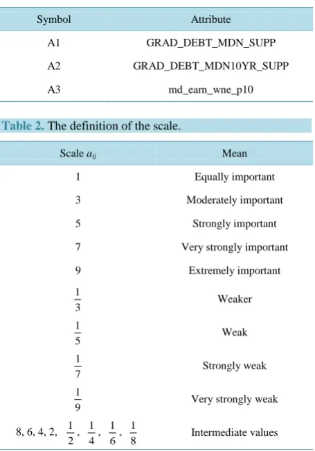
Three criterion include A1, A2 and A3 (Table 1). 2) Judgment Matrix
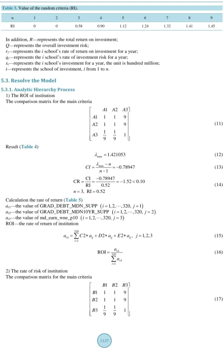
[image:5.595.201.429.216.373.2]Analyzing the same level of the relative importance of n indicators is completed by a number of experts. By 9 quintile ratio scale (Table 2).
[image:5.595.200.428.395.721.2]Figure 3. Hierarchy of criteria and sub-criteria.
Table 1. The full name of attributes and simplified symbols.
Symbol Attribute
A1 GRAD_DEBT_MDN_SUPP
A2 GRAD_DEBT_MDN10YR_SUPP
A3 md_earn_wne_p10
Table 2. The definition of the scale.
Scale aij Mean
1 Equally important
3 Moderately important
5 Strongly important
7 Very strongly important
9 Extremely important
1
3 Weaker
1
5 Weak
1
7 Strongly weak
1
9 Very strongly weak
8, 6, 4, 2, 1
2, 1 4,
1 6,
1
1) Each element (aij) of judgment matrix stands for the value of criterion i row and j column relative
impor-tance of pairwise comparisons. In judgment matrix,
(
)
1
0, 1, , 1, 2, ,
ij ij ij ji
a a a i j n
a
> = = = .
Below, a matrix constructed for 3 criterion is shown.
11 12 13
21 22 23
31 32 33
1 2 3
1 2 3
A A A
A a a a
A a a a
A a a a
(1)
2) Calculate the weight and consistency inspection
The literature contains calculations formulas for the subsequent steps leading to the calculation of the value of a priority criterion [5].
a) Calculations of the multiplication of each row element
1
, 1, 2, ,
n i ij
j
M a i n
=
=
∏
= . (2)b) Calculation of the root of Mi
n i i
W = M . (3) c) Normalized matrix:
T
1, 2, , n
w= W W W
1 i i n i n W w W = =
∑
w stands for weight. (4)d) The maximum characteristic root,
(
)
max 1 1 n i i i AW n w λ ==
∑
. (5)e) value of the consistency criterion:
max CI 1 n n λ − =
− . (6) f) consistency ratio:
CI CR
RI
= (7)
where the CR should reach a value <10%, (n > 2).
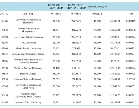
Finding the corresponding average random consistency criterion RI. For n = 1, 2, ∙∙∙, 9, Saaty [5] gives the value of RI. As shown in Table 3.
Model two. According to the maximum return on investment and the smallest investment risk, we want to seek the optimal investment scheme. We set up the following multi-objective risk investment model [6].
The objective function:
1
max
n i i i
R r x
=
=
∑
(8)1
min
n i i i
Q q x
=
=
∑
(9)1 1 . 0 n i i i x s t x = = ≥
Table 3. Value of the random criteria (RI).
n 1 2 3 4 5 6 7 8 9
RI 0 0 0.58 0.90 1.12 1.24 1.32 1.41 1.45
In addition, R—represents the total return on investment;
Q—represents the overall investment risk;
ri—represents the i school’s rate of return on investment for a year;
qi—represents the i school’s rate of investment risk for a year;
xi—represents the i school’s investment for a year, the unit is hundred million;
i—represents the school of investment, i from 1 to n.
5.3. Resolve the Model
5.3.1. Analytic Hierarchy Process 1) The ROI of institution
The comparison matrix for the main criteria
1 2 3
1 1 1 9
2 1 1 9
1 1
3 1
9 9
A A A
A A A (11)
Result (Table 4)
max 1.421053
λ = (12)
max 0.78947 1 n CI n λ − = = −
− (13) CI 0.78947
CR 1.52 0.10
RI 0.52
3, RI 0.52
n
−
= = = − <
= =
(14)
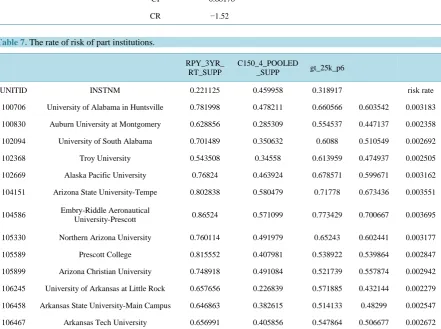
Calculation the rate of return (Table 5)
ai1—the value of GRAD_DEBT_MDN_SUPP
(
i=1, 2,, 320, j=1)
ai2—the value of GRAD_DEBT_MDN10YR_SUPP(
i=1, 2,, 320, j=2)
ai3—the value of md_earn_wne_p10(
i=1, 2,, 320, j=3)
ROI—the rate of return of institution
320
4 1
2 2 2 , 1, 2, 3
i ij ij ij i
a C a D a E a j
=
=
∑
∗ + ∗ + ∗ = (15)4 320 4 1 ROI i i i a a = =
∑
(16)2) The rate of risk of institution
The comparison matrix for the main criteria
1 2 3
1 1 1 9
2 1 1 9
1 1
3 1
9 9
B B B
Table 4. The ROI of institution.
A1 A2 A3 Mi Wi Weight
A1 1 1 9 9 2.080084 0.473684
A2 1 1 9 9 2.080084 0.473684
A3 1/9 1/9 1 0.01234568 0.23112 0.052632
4.391288
Check consistency
λmax 1.421053
CI −0.78947
[image:8.595.92.539.277.622.2]CR −1.52
Table 5. The rate of return of part institutions.
GRAD_DEBT_ MDN_SUPP
GRAD_DEBT_
MDN10YR_SUPP md_earn_wne_p10
UNITID INSTNM 0.473684 0.473684 0.052632 RIO
100706 University of Alabama in
Huntsville 24,738 274.6425 46,600 14,300.74 0.003419
100830 Auburn University at
Montgomery 21,791 241.9248 34,800 12,268.24 0.002938
102094 University of South Alabama 25,000 277.5513 38,300 13,989.38 0.003344
102368 Troy University 26,000 288.6533 36,600 14,378.85 0.003437
102669 Alaska Pacific University 25,125 278.939 47,400 14,528.2 0.003473
104151 Arizona State University-Tempe 20,375 226.2043 45,200 12,137.43 0.002901
104586 Embry-Riddle Aeronautical
University-Prescott 26,000 288.6533 60,900 15,657.8 0.003743
105330 Northern Arizona University 21,450 238.139 38,800 12,315.45 0.002944
105589 Prescott College 25,000 277.5513 35,200 13,826.22 0.003305
105899 Arizona Christian University 22,625 251.1839 31,000 12,467.67 0.00298
106245 University of Arkansas at Little Rock 23,000 255.3472 34,800 12,847.28 0.003071
106458 Arkansas State
University-Main Campus 20,959 232.6879 32,700 11,759.23 0.002811
106467 Arkansas Tech University 17,528 194.5967 35,000 10,237.03 0.002447
B1—stands for GRAD_DEBT_MDN_SUPP
B2—stands for GRAD_DEBT_MDN10YR_SUPP
B3—stands for md_earn_wne_p10 Result (Table 6)
max 1.636434
λ = (18)
max
CI 0.68178
1
n n
λ − = = −
CI 0.68178
CR 1.31 0.10
RI 0.52
3, RI 0.52
n
−
= = = − <
= =
(20)
Calculation the rate of risk (Table 7)
bi1—the value of GRAD_DEBT_MDN_SUPP
(
i=1, 2,, 320, j=1)
bi2—the value of GRAD_DEBT_MDN10YR_SUPP(
i=1, 2,, 320, j=2)
bi3—the value of md_earn_wne_p10(
i=1, 2,, 320, j=3)
I—the rate of risk
320
4 1
2 2 2 , 1, 2, 3
i ij ij ij i
b C b D b E b j
=
[image:9.595.93.535.387.716.2]=
∑
∗ + ∗ + ∗ = (21)Table 6. The rate of risk of institution.
B1 B2 B3 Mi Wi Weight
B1 1 3 1/9 0.33333333 0.693361 0.221125
B2 1/3 1 9 3 1.44225 0.459958
B3 9 1/9 1 1 1 0.318917
3.135611
Check consistency
λmax 1.636434
CI −0.68178
CR −1.52
Table 7. The rate of risk of part institutions.
RPY_3YR_ RT_SUPP
C150_4_POOLED
_SUPP gt_25k_p6
UNITID INSTNM 0.221125 0.459958 0.318917 risk rate
100706 University of Alabama in Huntsville 0.781998 0.478211 0.660566 0.603542 0.003183
100830 Auburn University at Montgomery 0.628856 0.285309 0.554537 0.447137 0.002358
102094 University of South Alabama 0.701489 0.350632 0.6088 0.510549 0.002692
102368 Troy University 0.543508 0.34558 0.613959 0.474937 0.002505
102669 Alaska Pacific University 0.76824 0.463924 0.678571 0.599671 0.003162
104151 Arizona State University-Tempe 0.802838 0.580479 0.71778 0.673436 0.003551
104586 Embry-Riddle Aeronautical
University-Prescott 0.86524 0.571099 0.773429 0.700667 0.003695
105330 Northern Arizona University 0.760114 0.491979 0.65243 0.602441 0.003177
105589 Prescott College 0.815552 0.407981 0.538922 0.539864 0.002847
105899 Arizona Christian University 0.748918 0.491084 0.521739 0.557874 0.002942
106245 University of Arkansas at Little Rock 0.657656 0.226839 0.571885 0.432144 0.002279
106458 Arkansas State University-Main Campus 0.646863 0.382615 0.514133 0.48299 0.002547
4 320 4 1 i i i b I b = =
∑
(22)5.3.2. Multi Objective Programming
Solving multi-objective problem is more difficult, so we need to convert them to more easily problem of a single target. Because of a variety of methods: The main objective method, linear weighted sum method, the weighted sum of squares method, ideal point method, multiplication and division, efficacy coefficient method, stepwise method, constraint method, etc. So, our team decided to use the most simple constraint method to solve it, which convert one of the goals to constraints conditions, while another goal will be goal function. Like this, Solving Multi-objective programming problem with two objectives will be transformed into solving a single [7].
Using the constraint method to following: The objective function:
1 1 1 max min . . 1 0 n i i i n i i i n i i i R Q
R r x
Q q x
s t x x = = = = = = ≥
∑
∑
∑
(23)In addition, R—represents the total return on investment;
Q—represents the overall investment risk;
ri—represents the i school’s rate of return on investment for a year;
qi—represents the i school’s rate of investment risk for a year;
xi—represents the i school’s investment for a year, the unit is hundred million US dollars;
i—represents the school of investment, i from 1 to 320.
According constraint equations listed above, calculated by the Analytic Hierarchy Process risk rate and rate of return, we can get a result. Because amount of data are so big, we use c language to solve. C language imple-mentation process is as follows:
In order to ensure the maximum return and minimum risk, so we consider the recursive iterative algorithm in the end. First, putting the results of the risk rate and rate of return on the txt file and write a program to reads file data. Secondly, putting program into two parts, one is to calculate max and min, another is to calculate the money of investment in every school. According to Iterative Algorithms, until the value from large to small equal value from small to large, the program is end [8].
The following procedure is recursive algorithm processes (Figure 4):
In a recursive algorithm, I advance its recursive algorithm, There are three aspects: First, each call will narrowed in size (usually the size is half);
Second, there is a close link between adjacent repeated twice, once time is prepare for the time after (usually output on a previous post is input);
Third, when a size of the problem is extremely small, you must be given directly to answer rather than a re-cursive call, so each rere-cursive call is conditional, unconditional rere-cursive calls will become died loop and not have a normal end.
By recursive algorithm, we got the investment for 320 schools.
6. Results and Analysis
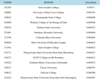
On the basis of solving process, we can get the following results:
Figure 4. Recursive algorithm.
Table 8. Part of the data for every school’s investment (Unit: Hundred Million US Dollars).
UNITID INSTNM Investment
152363 Saint Josephs College 0.00471
160065 Our Lady of Holy Cross College 0.004701
196042 Farmingdale State College 0.004698
392840 Watkins College of Art Design & Film 0.004696
228529 Tarleton State University 0.004672
221661 Southern Adventist University 0.004664
127556 Colorado Mesa University 0.004663
204820 Ohio University-Chillicothe Campus 0.004642
152363 Saint Josephs College 0.004623
214713 Pennsylvania State University-Penn State Harrisburg 0.004613
196237 SUNY College at Old Westbury 0.004612
149222 Southern Illinois University-Carbondale 0.004593
169327 Cleary University 0.004591
184612 Felician College 0.004588
214625 Pennsylvania State University-Penn State New Kensington 0.004567
3) The annual risk loss money on investment is 0.3128 million dollar.
4) The annual net return on investment is 59.3854 − 0.3128 = 59.0726 million dollar. 5) Forecasting total return on investment for the five-year is 295.363 billion dollar.
From the results, we can see that Goodgrant foundation invest 100 million on 320 schools. In the end of year, they can obtain 60% of repay money. The risk loss of investment for these schools will reduce year by year. The repay on investment will be stable in the fifth year, the overall return on investment in five years will reach 60% of the total investment. The most important thing is that schools obtain the investment within five years will im-prove largely comprehensive capabilities and students’ ability in these schools will have greatly imim-proved too.
7. Strengths and Weaknesses
7.1. Strengths
[image:11.595.143.484.266.537.2]2) We developed a theoretical line formation model which agrees without rough data. Our computer model agrees with both despite working on different principles, implying it behaves as we want.
3) This main model allows us to make substantive conclusions.
4) The fundamental strengths of our model are its robustness and flexibility. All of the data is fully paramete-rized, so the model can be applied to solve practical problems.
7.2. Weaknesses
Some special data can’t be found, and it makes that we have to do some proper assumption before the solution of our models. A more abundant data resource can guarantee a better result in our models. Current line length is not taken into account by the line formation model. In real life, it’s not so ideal.
References
[1] Šelih, J., Kne, A., Srdi, A. and Žura, M. (2008) Multiple-Criteria Decision Support System in Highway Infrastructure Management. Transport, 23, 299-305.http://dx.doi.org/10.3846/1648-4142.2008.23.299-305
[2] Cao, M.L. (2012) Analytic Hierarchy Process (AHP) to Determine Evaluation Criteria Weights and Excel Calculation.
Science and Technology Information of Jiangsu, 2, 39-40.
[3] Xiao, F.H. (2014) AHP in the Application of the Construction Project Settlement Audit Tender and Bid Evaluation in Colleges and Universities. China Science and Technology Information, 4, 21-23.
[4] Jing, W., De Yu, Y. and Mei Li, D. (2015) Application of Analytic Hierarchy Process (AHP) in the Student Employ-ment Choice. Horizon of Science and Technology, 6, 141-144.
[5] Yuan, J. (2013) Investment Income Research Institutions of High Education Foundation. Nanjing University of Aero-nautics and AstroAero-nautics.
[6] Lv, X., Xu, S.Y. and Zhang, G. (1999) The Mathematical Model of Portfolio Investment. Journal of Harbin Institute of Technology University, 4, 51-54.
[7] Lin, W. (2015) High Education in the United States Return Questions under the Knowledge Economy. Education Re-search.
[8] Zheng, B.L. (2016) The Recursive and Iterative Algorithm and Its Application in the JAVA Language. Information and Computer (Theory).