Inducing Probabilistic Relational Rules from Probabilistic Examples
∗Luc De Raedt, Anton Dries, Ingo Thon
†, Guy Van den Broeck, Mathias Verbeke
‡KU Leuven, Department of Computer Science
Celestijnenlaan 200A, BE-3001 Heverlee, Belgium
Abstract
We study the problem of inducing logic programs in a probabilistic setting, in which both the example descriptions and their classification can be bilistic. The setting is incorporated in the proba-bilistic rule learner ProbFOIL+, which combines principles of the rule learner FOIL with ProbLog, a probabilistic Prolog. We illustrate the approach by applying it to the knowledge base of NELL, the Never-Ending Language Learner.
1
Introduction
Motivated by the interest in probabilistic logic learning [De Raedtet al., 2008; De Raedt and Kimmig, 2013], and sta-tistical relational learning (SRL) [Getoor and Taskar, 2007], we revisit the classical rule learning problem, but focus on a probabilistic instead of the classical deterministic setting pursued in inductive logic programming (ILP). Compared to inductive logic programming and traditional rule learners, we study an upgraded setting in which Prolog is replaced by a probabilistic Prolog, called ProbLog, and in which the rules, background theory and examples are allprobabilisticrather than deterministic. The upgraded setting has the property that when all probabilities are set to 0 and 1, it corresponds to the standard ILP problem, as addressed by FOIL [Quinlan, 1990] and Progol [Muggleton, 1995].
In probabilistic rule learning, the task is to learn rules from examples that have both a probabilistic description and a probabilistic classification. In terms of ILP, this means that all atoms in the example description and target atom have a probability. The learned rules are used for predicting the probability of the target predicate (the output) given the prob-abilities in the description of the example (the inputs). This prediction task differs from standard rule-learning and ILP in that the hypotheses generated by ILP systems require the inputs to be deterministic and usually the prediction as well (although some rule-learners output the confidence of their prediction). In SRL systems, on the other hand, it is possi-ble to provide probabilistic inputs and make a probabilistic
∗
All authors contributed equally to this work. †
Now at Siemens AG, Otto-Hahn-Ring 6, GE-81739 Munich ‡
Now at Sirris, A. Reyerslaan 80, BE-1030 Brussels
prediction for a specific example. However, SRL systems do not learn rules or structure from probabilistic examples and they also do not upgrade the traditional rule learning or ILP setting, see Section 5 for more details.
The probabilistic rule learning setting is useful in any situ-ation in which both the example descriptions and their classi-fication are probabilistic (or uncertain). This arises naturally when example descriptions are produced through perception. For instance, in vision or autonomous agents, the example description can be the image description or the belief state, which is often produced using components that have been learned themselves to detect certain objects, relationships or measurements and which typically also indicate the reliability of the description. Similarly, when crawling and parsing the web, one obtains descriptions or parses of the involved texts that are uncertain themselves. Yet in all these situations it can be beneficial to learn rules that capture interrelationships between the predicates and that allow to predict in a reliable way particular target predicates. We shall illustrate this in the context of NELL, the Never-Ending Language Learner [Carl-sonet al., 2010]. Probabilistic rule learning applies also nat-urally to probabilistic databases, which consist by definition of probabilistic facts. As two final examples, let us mention the work by [Chenet al., 2008], who argue that probabilistic examples arise naturally when performing scientific experi-ments as the outcome of experiexperi-ments may be uncertain, and a medical scenario in which doctors may describe all they know about a particular patient in terms of (subjective) prob-abilities. As such they might provide, in addition to some de-terministic descriptions, statements about their belief in the outcome of an expensive test on a patient as well as their be-lief that the patient will survive the next five years.
We contribute an integrated approach to learning proba-bilistic relational rules from probaproba-bilistic examples and back-ground knowledge. It is incorporated in the ProbFOIL+ sys-tem and builds on ProbLog [De Raedtet al., 2007], a simple probabilistic Prolog, and FOIL [Quinlan, 1990], and employs well-known principles and heuristics of rule learning [Lavrac et al., 2012]. The key contributions of ProbFOIL+ are 1) that it upgrades a traditional inductive logic programming system towards a probabilistic setting, in which the exam-ple descriptions, targets and learned rules are all probabilis-tic, 2) that the predicted probability for a target instance is the probability with which the instance is true (the degree of
be-lief), 3) that it tightly integrates the rule and weight learning in a one-step process, rather than learning these separately, and 4) that it efficiently computes the probability of candi-date clauses, without resorting to an expensive optimization approach, which is enabled by combining the traditional se-quential covering approach with a local optimization step to compute the weights. ProbFOIL+differs significantly from existing SRL approaches as we shall argue in Section 5.
This paper is organized as follows. We define the prob-abilistic rule learning problem in Section 2. Section 3 de-scribes ProbFOIL+1, our algorithm for learning probabilistic
rules from probabilistic data. In Section 4 our approach is evaluated with a case study on NELL, the Never-Ending Lan-guage Learner [Carlsonet al., 2010]. An overview of related work can be found in Section 5, and conclusions in Section 6.
2
Background and Problem Specification
We first introduce basic concepts of logic programming (Pro-log). Anatomp(t1,· · ·, tn)consists of apredicatep/nof ar-itynandtermst1,· · · , tn. A term is a (lowercase)constant, an (uppercase)variable, or afunctor. Aliteralis an atom or its negation. Aclauseis a conjunction of literals. Adefinite clausecontains exactly one non-negated atom, and is denotedh ← b1,· · ·, bn. The headhand the bodyb1,· · ·, bn con-sists of atomsh, bi. Asubstitutionθ={V1/t1,· · ·, Vm/tm} maps variablesVito termsti. Applyingθto an atoma, de-notedaθ, replaces all occurrences ofViinabyti. A ground-ing substitutionremoves all logical variables.
ProbLog is a probabilistic Prolog that allows one to work with probabilistic facts and background knowledge [De Raedt et al., 2007]. A ProbLog program consists of a set of definite clauses D and a set of probabilistic facts
pi :: ci, which are facts ci labeled with the probability
pi that their ground instances ciθ are true. Given a fi-nite set of grounding substitutions {θj1, . . . θjij} for each probabilistic fact pj :: cj, consider the set of ground factsLT = {c1θ11, . . . , c1θ1i1,· · ·, cnθn1, . . . , cnθnin}. A ProbLog programT ={p1::c1, ..., pn::cn}defines a prob-ability distribution over subsets of factsL⊆LT as
P(L|T) =Y ciθj∈L pi Y ciθj∈LT\L (1−pi). In combination with the clausesD, ProbLog then defines the success probabilityof a queryqto be
Ps(T |=q) =
X
L⊆LT L∪D|=q
P(L|T).
In other words, the probability ofqis the probability thatq
isentailedusing the background knowledge together with a random set of ground probabilistic facts.
Definition 1 (Probabilistic Rule Learning)Given:
1. a set of examplesE, consisting of pairs(xi, pi), where
xi is a ground fact for the unknown target predicatet andpiis a target probability;
1
ProbFOIL+ and the datasets used in this paper in ProbFOIL+ format can be downloaded from https: //dtai.cs.kuleuven.be/software/probfoil/.
2. a background theory B containing information about the examples in the form of a ProbLog program; 3. a loss functionloss(H, B, E), measuring the loss of a
hypothesis (set of clauses)Hw.r.t.BandE;
4. a space of possible clausesLhspecified using a declar-ative bias;
Find: A hypothesis H ⊆ Lh such that H = arg minHloss(H, B, E).
This loss function aims at minimizing the standard error of the predictions, that is,loss(H, B, E) =P
(xi,pi)∈E|Ps(B∪
H|=xi)−pi|. It is a simple choice with the benefit that well-known concepts and notions from rule learning and classifica-tion directly carry over to the probabilistic case. Furthermore, this loss function is also used in Kearns and Schapire’s prob-abilistic concept-learning framework [Kearns and Schapire, 1994], a generalization of Valiant’s probably approximate correct learning framework to predicting the probability of examples rather than their class. The above definition gen-eralizes that framework further by assuming that also the de-scriptions of the examples themselves are probabilistic, not just their classes.
Notice that this problem setting generalizes both traditional rule learning and ILP to a probabilistic setting. To see this, consider that in the original FOIL system, the background theory was specified as a set of ground facts{fj}and each example was a true or false fact for the target predicate xi. In the present setting, the background theory consists of a set of probabilistic facts {pj :: fj} (possibly together with a set of definite clauses) and the examples (xi, pi)are also labelled with their target probability. It should be clear that the original setting is obtained when all probabilitiespjand
pi are 0 or 1. This is in line with the theory of probabilistic logic learning [De Raedt, 2008]. The ILP setting obtained is that of learning from entailment because examples are facts that are entailed by the theory.
This problem setting was proposed initially in De Raedt and Thon [2010], where also a preliminary rule-learner called ProbFOIL was proposed and illustrated at work on two toy examples. Both the setting and the rule learner pre-sented in the current paper extend the work of De Raedt and Thon [2010] as we account for probabilistic rules (of the form
x :: head ← body) instead of the deterministic ones (with
x = 1) in ProbFOIL, we determine the optimal weightsx
(cf. Section 3), and include an experimental evaluation using Bayesian networks and NELL, cf. Section 5.
3
ProbFOIL
+Algorithm Our ProbFOIL+algorithm for learning proba-bilistic clauses is shown as Algorithm 1. It directly general-izes the mFOIL rule learner, and closely resembles the vanilla rule-learning algorithm (cf. Mitchell [1997]) in that it follows the typical sequential covering approach. The outer loop of the algorithm starts from an empty set of clauses and repeat-edly adds clauses to the hypothesis until no more improve-ment is observed with respect to aglobal scoring function. The clause to be added is obtained by the function LEARN
-RULE, which greedily searches for the clause that maximizes alocal scoring function, using the refinement operatorρ.
Algorithm 1The ProbFOIL+learning algorithm. 1: functionPROBFOIL+(target)
2: H:=∅
3: whiletruedo
4: clause :=LEARNRULE(H,target)
5: if GSCORE(H)<GSCORE(H∪ {clause})then
6: H:=H∪ {clause}
7: else returnH
8: functionLEARNRULE(H,target) 9: candidates:={x::target←true}
10: best:= (x::target←true)
11: whilecandidates6=∅do
12: next cand:=∅
13: for allx::target ←body∈candidatesdo
14: for allrefinement∈ρ(target←body)do
15: ifnot REJECT(H,best,x::target←body)then
16: next cand:=next cand∪ {x::target←body∧
17: refinement}
18: ifLSCORE(H,x::target←body∧refinement)>
19: LSCORE(H,best)then
20: best := (x::target←body∧refinement)
21: candidates :=next cand 22: returnbest
While ProbLog and Prolog assume that the rules are def-inite clauses, in ProbFOIL+ we use probabilistic rules of the form x :: target ← body. This is short hand for a ProbLog program with the deterministic rule target ←
body∧prob(id)and probabilistic factx:: prob(id), where
id is an identifier that refers to this particular rule. Notice that all facts for such rules are independent of one another, and also that the probabilityxwill have to be determined by the rule learning algorithm. Each call to LSCOREreturns the best score that can be achieved for any value ofx, and when returning the best found rule in line 22, the value ofxis fixed to the probability that yields the highest local score.
Scoring Functions ProbFOIL+ uses (upgraded versions) of standard scoring functions for rule learning, though oth-ers can easily be adapted as well. As the global scoring function, which determines the stopping criterion of the outer loop, we use accuracyH = TPH+MTNH where M is the size of the dataset. The local scoring function is based on the m-estimate, a variant of precision that is more ro-bust against noise in the training data, which is defined as
m-estimateH =
TPH+mNP+P
TPH+FPH+m,wheremis a parameter of the algorithm, andPandNindicates the number of positive and negative examples in the dataset, respectively.
Both these metrics are based on the number of examples correctly classified as positive (true positives, TP) and the number of examples incorrectly classified as positive (false positives, FP), which form the basis of the contingency ta-bles for classification, and which we now upgrade for use in a probabilistic setting. While in a deterministic setting, each exampleei has a 1/0 target classification, this now be-comes a probability value pi. This means that every
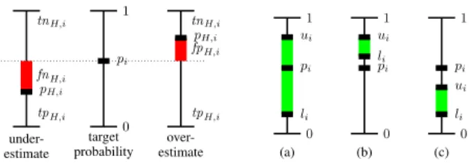
ex-pH,i tnH,i fnH,i tpH,i 1 0 pi pH,i tnH,i fpH,i tpH,i under-estimate target probability over-estimate 1 0 ui pi li 1 0 ui li pi 1 0 pi ui li (a) (b) (c)
Figure 1: True/false and pos./neg. parts of a single example (left). Values forli,uiandpi where (a) it is still possible to perfectly predictpiwith the right value forx, or wherepiwill always be (b) overestimated or (c) underestimated (right).
ample contributes pi to the positive part of the dataset and 1 −pi to the negative part of the dataset, which general-izes the deterministic setting with pi = 1 for positive and
pi = 0for negative examples. In general, we define the pos-itive and negative parts of the dataset asP = PM
i=0pi and
N =PM
i=0(1−pi) =M−P.
The same approach generalizes the predictions of a model to the probabilistic setting where a hypothesis H will pre-dict a valuepH,i ∈ [0,1]for example ei instead of0 or 1. In this way we can define a probabilistic version of the true positive and false positive rates of the predictive model as
TPH = P M
i=0tpH,i, wheretpH,i = min(pi, pH,i) and
FPH =P M
i=0fpH,i, wherefpH,i= max(0, pH,i−pi).For completeness we note thatTNH =N−FPHandFNH =
P−TPH, as was the case in the deterministic setting. Figure 1 illustrates these concepts. If a hypothesisH over-estimates the target value ofei, that is,pH,i > pi then the true positive parttpi will be maximal, that is, equal to pi. The remaining part,pH,i−pi, is part of the false positives. If
Hunderestimates the target value ofeithen the true positive part is onlypH,iand the remaining part,pi−pH,icontributes to the false negative part of the prediction.
Calculatingx Algorithm 1 builds a set of clauses incre-mentally. Given a set of clauses H, it will search for the clausec(x) = (x::c)that maximizes the local scoring func-tion, wherex∈[0,1]is a multiplier indicating the probabil-ity that the body ofcentails its head. The local score of the clausecis obtained by selecting the best possible value forx, that is, we want to findarg maxxM(x)with
M(x) = TPH∪c(x)+m P N+P
TPH∪c(x)+FPH∪c(x)+m Next, we describe how to efficiently compute this value.
To find this optimal value, we need to be able to express the contingency table ofH∪c(x)in function ofx. As before, we usepito indicate the target value of exampleei.
We see thatpH∪c(x),iis a monotone function inx, that is, for each example ei and each value ofx,pH∪c(x),i ≥ pH,i and for each x1 and x2, such that x1 ≤ x2, it holds that
pH∪c(x1),i ≤ pH∪c(x2),i. The minimum and maximum pre-diction ofH∪c(x)for the exampleeiis thus
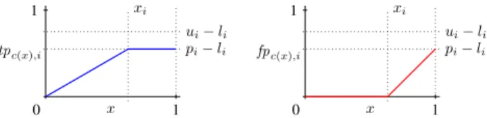
1 x 0 1 tpc(x),i xi ui−li pi−li 1 x 0 1 fpc(x),i xi ui−li pi−li
Figure 2: True and false positive rate for a single example
ei∈E3whereli< pi< ui.
Note thatuiis the prediction that would be made by the orig-inal ProbFOIL algorithm [De Raedt and Thon, 2010], which learns deterministic rules.
For each exampleei, we can decompose tpH∪c(x),i and
fpH∪c(x),iin
tpH∪c(x)=tpH,i+tpc(x),i fpH∪c(x),i=fpH+fpc(x),i,
wheretpc(x),iandfpc(x),iindicate the additional contribution of clausec(x)to the true and false positive rates.
Second, we divide the examples into three categories, as depicted in Figure 1:
E1: pi ≤li, i.e., the clausesoverestimatethe target value for this example, irrespective of the value ofx. For such an exampletpc(x),i= 0andfpc(x),i=x(ui−li).
E2: pi ≥ui, i.e., the clausesunderestimatethe target value for this example, irrespective of the value ofx. For such an exampletpc(x),i=x(ui−li)andfpc(x),i= 0.
E3: li < pi < ui, i.e., there exists a value ofxfor which the clause predicts the target value for this example per-fectly. We call this valuexiand it can be computed as
xi=
pi−li
ui−li
.
Figure 2 shows the values oftpc(x),iandfpc(x),iin func-tion ofx. The formulae for these functions are
tpc(x),i= x(ui−li) ifx≤xi, pi−li ifx > xi and fpc(x),i= 0 ifx≤xi, x(ui−li)−(pi−li) ifx > xi .
We can now determine the contribution to TPc(x) and
FPc(x)of the examples in each of these categories. For the examples inE1, the contributions toTPc(x)andFPc(x)are
TP1(x) = 0andFP1(x) =x E1
X
i
(ui−li) =xU1.
For the examples in E2, the contribution to TPc(x) and
FPc(x)are TP2(x) =x E2 X i (ui−li) =xU2andFP2(x) = 0.
For the examples in E3, the contributions to TPc(x) and
FPc(x)are TP3(x) =x E3 X i:x≤xi (ui−li)+ E3 X i:x>xi (pi−li) =xU3≤xi+P >xi 3 , FP3(x) =x E3 X i:x>xi (ui−li)− E3 X i:x>xi (pi−li) =xU3>xi−P >xi 3 . By using the fact that TPH∪c(x) = TPH +TP1(x) +
TP2(x) +TP3(x) and FPH∪c(x) = FPH +FP1(x) +
FP2(x) +FP3(x)and by reordering terms we can reformu-late the definition of the m-estimate as
M(x) = TPH∪c(x)+m P N+P TPH∪c(x)+FPH∪c(x)+m =(U2+U ≤xi 3 )x+TPH+P3>xi+mNP+P (U1+U2+U3)x+TPH+FPH+m . (1) In the last step we replacedFP3(x)+TP3(x) =xP
E3 i (ui− li) =xU3. By observing thatU≤xi 3 andP >xi
3 are constant on the in-terval between two consecutive values ofxi, we see that this function is a piecewise non-linear function where each seg-ment is of the form
Ax+B Cx+D
whereA, B, CandDare constants. The derivative of such a function is
dM(x)
dx =
AD−BC
(CX+D)2,
which is non-zero everywhere or zero everywhere. This means that the maximum of M(x) will occur at one of the endpoints of the segments, that is, in one of the points
xi. By incrementally computing the values of U3≤xi =
PE3 i:x≤xi(pi−li)andP >xi 3 = PE3 i:x>xi(pi−li)in Equation 1 for thexi in increasing order, we can efficiently find the value ofxthat maximizes the local scoring function. More-over, by computing one probabilityui = pH∪c(1),i for each exampleei, we can obtain all probabilities for differentx, as
pH∪c(x),i=li+x(ui−li).
Significance In order to avoid learning large hypotheses with many clauses that only have limited contributions, we use a significance test. This test was also used in the mFOIL algorithm [Dˇzeroski, 1993]. It is a variant of the likelihood ratio statistic and is defined as
LhR(H, c) = 2(TPH,c+FPH,c)
precH,clog precH,c
prectrue+ (1−precH,c) log
1−precH,c 1−prectrue , where TPH,c=TPH∪c−TPH, FPH,c=FPH∪c−FPH
precH,c =
TPH,c
TPH,c+FPH,c
, prectrue= P
P+N.
This statistic is distributed according toχ2with one degree of freedom. Note that we use a relative likelihood, which is based on the additional prediction made by adding clausec
to hypothesisH. As a result, later clauses will automatically achieve a lower likelihood.
Local stopping criteria When we analyze the algorithm above, we notice that in the outer loop, the number of pos-itive predictions increases. This means that the values in the first row of the contingency table can only increase (and the values in the second row will decrease). More formally:
Property 1 For all hypotheses H1, H2: H1 ⊂ H2 →
TPH1 ≤TPH2andFPH1 ≤FPH2.
Additionally, in the inner loop, we start from the most gen-eral clause (i.e., the one that always predicts1), and we add literals to reduce the coverage of negative examples. As a result, the positive predictions will decrease.
Property 2 For all hypothesesH and clausesh←l1, ..., ln and literalsl:TPH∪{h←l1,...,ln}≤TPH∪{h←l1,...,ln,l}and
FPH∪{h←l1,...,ln}≤FPH∪{h←l1,...,ln,l}
We can use these properties to determine when a refine-ment can be rejected (line 15 of Algorithm 1). In order for a clause to be a viable candidate it has to have a refinement that 1) has a higher local score than the current best rule, 2) has a significance that is high enough (according to a preset threshold), and 3) has a better global score than the current rule set without the additional clause.
Implementation Details As usual in ILP, ProbFOIL+uses a declarative bias based on modes [Muggleton, 1995]. These specify syntactic restrictions on the clauses of interest and are used by the refinement operator during the search process.
The LEARNRULEfunction of the ProbFOIL+algorithm is based on mFOIL [Dˇzeroski, 1993] and uses a beam search strategy in order to escape from local maxima. It uses rela-tional path finding [Onget al., 2005; Richards and Mooney, 1992] to generate clauses by considering the connections be-tween the variables in the example literals, a proven technique to direct the search in first-order rule learning.
ProbFOIL+ computes the probabilities pH,i using the ProbLog2 system [Fierenset al., 2014].2 The ProbLog2
in-ference engine computes the probability of queries in four phases: it grounds out the relevant part of the probabilistic program, converts this to a CNF form, performs knowledge compilation into d-DNNF form and, finally, computes the probability from the obtained d-DNNF structure. This pro-cess is described in detail in [Fierenset al., 2014].
Due to the specific combinations and structure of ProbFOIL+’s queries, we can apply multiple optimizations3: Incremental groundingWhile the standard ProbLog2 would
2http://dtai.cs.kuleuven.be/problog/ 3
The remainder of the section can be skipped by the reader less familiar with probabilistic programming
perform grounding for each query, ProbFOIL+ uses incre-mental grounding techniques and builds on the grounding from the previous iteration instead of starting from scratch. This is possible as the rules are constructed and evaluated one literal at-a-time.
Direct calculation of probabilitiesBecause of the incremental nature of ProbFOIL+’s evaluation, we can often directly com-pute probabilities without having to resort to (costly) knowl-edge compilation, for example when we add a literal whose grounding does not share facts with the grounding of the rest of the theory (for which we computed the probability in a pre-vious iteration). This can also significantly reduce the size of the theories that need to be compiled.
Propositional dataWhen propositional data is used, all ex-amples have the same structural component. This means we can construct a d-DNNF for a single example and reuse it to evaluate all other examples.
Range-restricted rulesSince in a number of cases, it is desired that the result in rules arerange-restricted, i.e., that all vari-ables appearing in the head of a clause also appear in its body, ProbFOIL+ offers an option to output only range-restricted rules.
4
Experiments
We answer two questions experimentally.
Q1: How do ProbFOIL and ProbFOIL+compare to
stan-dard regression learners in the propositional case? This question is motivated by the observation that – in the propo-sitional case – the task can be viewed as that of predicting the probability of the target example from a set of probabilistic at-tributes, which can be solved by applying standard regression tasks. Of course, one then obtains regression models, which do not take the form of a set of logical rules that are easy to interpret. While regression can in principle be applied to the propositional case, it is hard to see which regression systems would apply to the relational case. The reason is that essen-tiallyall predicates are probabilistic (and hence, numeric), a situation that is – to the best of the authors’ knowledge – unprecedented in relational learning. Standard relational re-gression algorithms are able to predict numeric values start-ing from a relational description, a set of true and false ground facts. The goal of this experiment is not to suggest that prob-abilistic rule learning can contribute to regression, it is rather that regression provides a reasonable baseline that allows to evaluate the performance of probabilistic rule-learning.
Dataset We will generate data from Bayesian networks, both for dependent and independent attributes, and partial and full observability. Thetarget variablewill be the variable one wants to predict, this will always be a node that does not have children in the network. The evidence or descriptor variables will be a subset of the other variables.We use BNGenerator4
to randomly generate a Bayesian network structure. The con-ditional probability tables (CPT) and marginal distributions
4
http://www.pmr.poli.usp.br/ltd/Software/ BNGenerator/
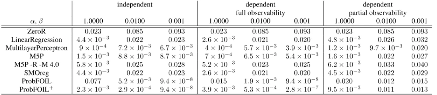
Table 1: Mean absolute error on the Bayesian network with CPTs∼Beta(α, β), averaged over all target attributes.
independent dependent dependent
full observability partial observability
α,β 1.0000 0.0100 0.001 1.0000 0.0100 0.001 1.0000 0.0100 0.001 ZeroR 0.023 0.085 0.093 0.023 0.085 0.093 0.023 0.085 0.093 LinearRegression 4.4×10⁻³ 0.022 0.023 2.6×10⁻³ 0.021 0.020 4.8×10⁻³ 0.026 0.032 MultilayerPerceptron 9×10⁻⁴ 7.2×10⁻³ 6.7×10⁻³ 4×10⁻⁴ 5.7×10⁻³ 3.9×10⁻³ 1.2×10⁻³ 9.7×10⁻³ 0.020 M5P 1.5×10⁻³ 8.8×10⁻³ 8.7×10⁻³ 7×10⁻⁴ 6.5×10⁻³ 5.4×10⁻³ 1.6×10⁻³ 0.022 0.027 M5P -R -M 4.0 5.8×10⁻³ 0.025 0.028 5.2×10⁻³ 0.023 0.025 6.2×10⁻³ 0.033 0.040 SMOreg 4.4×10⁻³ 0.022 0.023 2.6×10⁻³ 0.021 0.020 4.5×10⁻³ 0.022 0.029 ProbFOIL 0.077 5.2×10⁻³ 9.4×10⁻⁸ 0.015 1.9×10⁻³ 9.4×10⁻⁸ 0.020 0.012 0.015 ProbFOIL+ 2.3×10⁻³ 2.9×10⁻⁴ 9.4×10⁻⁸ 3.9×10⁻³ 5.3×10⁻⁴ 2.8×10⁻⁷ 9.5×10⁻³ 0.011 0.013
are left unspecified. The generated network has 45 nodes, 70 edges, a maximal degree of 6 and an induced width of 5.
Subsequently, different instances of the Bayesian network are generated by sampling its CPTs from a beta distribution Beta(α, β). Lower values for αand β make the network more “deterministic” and less “probabilistic”. To generate training and test examples for a single network instance, we uniformly sample marginal probabilities for the root nodes. These values, together with the inferred probability of the target, make up a single example. Each combination of tar-get attribute and beta distribution is a different learning prob-lem. For each of these, we trained ProbFOIL, ProbFOIL+ and standard regression learners from the Weka suite on 500 training examples. The learned models are evaluated on 500 test examples using the mean absolute error, which is 1 mi-nus the accuracy in the rule learning setting. We consider also three settings, whose results are shown in Table 1:
1. Independent Attributes. In this simplest setting, the ob-served attributes are all root nodes of the Bayesian net-work, i.e., a node with no parent nodes in the graph. 2. Dependent Attributes, Full Observability.In this setting,
the observed nodes are no longer the root nodes. Conse-quently, their probabilities are not independent anymore. There is, however, an observed node on every path from a root node to a target node, allowing for full observ-ability and the possibility of rediscovering the model the data was drawn from.
3. Dependent Attributes, Partial Observability. By drop-ping full observability, we can no longer learn the per-fect model.
Answer to Q1: In almost all cases ProbFOIL+performs on par or outperforms the standard regression learners, which demonstrates its advantage for propositional probabilistic rule learning. Furthermore, in all cases, similar or better results are obtained by ProbFOIL+when compared to Prob-FOIL, illustrating the added value of learning probabilistic rules with weights.
Q2: How does ProbFOIL+ perform for relational
prob-abilistic rule learning in the context of a probprob-abilistic knowledge base? The task to extract information from unstructured or semi-structured documents has recently at-tracted an increased amount of attention in the context of
Ma-Table 2: Number of facts per predicate (NELL sports dataset) for predicates used in the learned rules (Table 3).
athleteledsportsteam(athlete,team) 246 athleteplaysforteam(athlete,team) 808 athleteplaysinleague(athlete,league) 1197 athleteplayssport(athlete,sport) 1899 teamalsoknownas(team,team) 273 teamplaysagainstteam(team,team) 2848 teamplayssport(team,sport) 340 teamplaysinleague(team,league) 1229
chine Reading. Here we focus on NELL5, to which several rule learning approaches have already been applied, as dis-cussed in Section 5.
Dataset In order to test probabilistic rule learning for NELL, we extracted the facts for all predicates related to the sports domain from iteration 850 of the NELL knowledge base6. A similar dataset was used in the
con-text of meta-interpretive learning [Muggleton and Lin, 2013]. Our dataset contains 10567 facts. The number of facts per predicate (and their types) are listed in Table 2. Each fact has a probability value attached (e.g., 0.934 ::
athleteplaysf orteam(thurman thomas, buf f alo bills)). Part of the negative examples are the negative contribution of the positive examples (1−probability). The additional neg-ative examples are generated by taking random combinations of constants present in the dataset (while respecting the type information). To reduce the search space during rule learn-ing, we impose the constraint that each literal can introduce at most one new variable as well as range-restrictedness.
To evaluate ProbFOIL+ in the context of NELL, we learned rules for each binary predicate7with more than 500 facts. In order to have a reasonable number of examples per fold, we used 3-fold cross-validation. To create the folds, for each target predicate, the facts were randomly split into 3 parts. Each fold consists of all non-target predicates and a
5
Seehttp://rtw.ml.cmu.edu
6
Fromhttp://rtw.ml.cmu.edu/rtw/resources. It-eration 850 was the last available itIt-eration at the time of experimen-tation.
7
Note that for the presented algorithm, the target predicates are not restricted to binary only. This just happens to be the case in the dataset we use.
Table 3: Learned relational rules for the different predicates (fold 1). 0.9375::athleteplaysforteam(A,B) ← athleteledsportsteam(A,B).
0.9675::athleteplaysforteam(A,B) ← athleteledsportsteam(A,V1), teamplaysagainstteam(B,V1). 0.9375::athleteplaysforteam(A,B) ← athleteplayssport(A,V1), teamplayssport(B,V1).
0.5109::athleteplaysforteam(A,B) ← athleteplaysinleague(A,V1), teamplaysinleague(B,V1).
0.9070::athleteplayssport(A,B) ← athleteledsportsteam(A,V2), teamalsoknownas(V2,V1), teamplayssport(V1,B), teamplayssport(V2,B).
0.9070::athleteplayssport(A,B) ← athleteplaysforteam(A,V2), teamalsoknownas(V2,V1), teamplayssport(V1,B), teamplayssport(V2,B),teamalsoknownas(V1,V2).
0.9070::athleteplayssport(A,B) ← athleteplaysforteam(A,V1), teamplayssport(V1,B). 0.9286::athleteplaysinleague(A,B) ← athleteledsportsteam(A,V1), teamplaysinleague(V1,B).
0.7868::athleteplaysinleague(A,B) ← athleteplaysforteam(A,V2), teamalsoknownas(V2,V1), teamplaysinleague(V1,B). 0.9384::athleteplaysinleague(A,B) ← athleteplayssport(A,V2), athleteplayssport(V1,V2), teamplaysinleague(V1,B). 0.9024::athleteplaysinleague(A,B) ← athleteplaysforteam(A,V1), teamplaysinleague(V1,B).
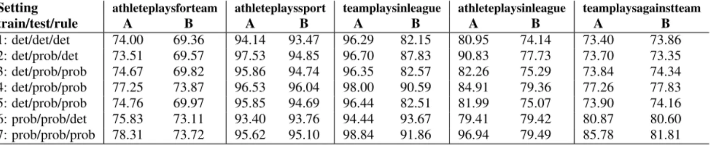
Table 4: Precision for different experimental setups and parameters (A:m= 1, p= 0.99,B:m= 1000, p= 0.90).
Setting athleteplaysforteam athleteplayssport teamplaysinleague athleteplaysinleague teamplaysagainstteam
train/test/rule A B A B A B A B A B 1: det/det/det 74.00 69.36 94.14 93.47 96.29 82.15 80.95 74.14 73.40 73.86 2: det/prob/det 73.51 69.57 97.53 94.85 96.70 87.83 90.83 77.73 73.70 73.35 3: det/prob/prob 74.67 69.82 95.86 94.74 96.35 82.57 82.26 75.29 73.84 74.34 4: det/prob/prob 77.25 73.87 96.53 96.04 98.00 90.59 84.91 79.36 77.26 77.83 5: det/prob/prob 74.76 69.97 95.85 94.69 96.44 82.51 81.99 75.07 73.90 74.16 6: prob/prob/det 75.83 73.11 93.40 93.76 94.44 93.67 79.41 79.42 80.87 80.60 7: prob/prob/prob 78.31 73.72 95.62 95.10 98.84 91.86 96.94 79.49 85.78 81.81
part of the target predicates. Due to space limitations, we only report the rules for three of the predicates that are learned on the first fold. Similar rules were obtained on the other predi-cates and folds.
Experimental set-up. Our experimental set-up is moti-vated as follows. As baselines for probabilistic rule learn-ing, we chose several special cases of ProbFOIL+, possibly combined with other techniques. Each of these special cases closely corresponds to an approach that exists in the litera-ture, and hence, can be used as a baseline. This provides a more controlled experimental setting than a comparison with other ILP or SRL systems. Furthermore, a comparison with other ILP or SRL systems would be problematic as we are not aware of other systems that can cope with both probabilis-tic descriptions and probabilisprobabilis-tic classifications. In addition, when considering, for instance, Markov Logic, it would be unclear how to turn the probabilities of atoms in the example descriptions into weights for use by Markov Logic.
Setting 1 is the fully deterministic case. If ProbFOIL+ uses fully deterministic examples, this directly corresponds to mFOIL and thus is representative of the pure ILP approach. To this end, as usual in NELL, we interpret each example with a probability higher than 0.75 as a positive one, and each ex-ample with a lower probability as a negative one. Setting 2 uses the same learning algorithm and data as in Setting 1 but uses the learned rules with probabilistic inputs to produce a probabilistic classification. Setting 3 is a variant of Setting 1 in which we first learn the rules in a purely deterministic way (as in Settings 1 and 2), and then assign a weight to each
learned rule. The weight is the precision of the rule estimated using the probabilities of the target in the training set. This closely corresponds to what some rule and decision tree learn-ers do, namely estimating the probability of class memblearn-ership in the conclusion part of the rule or in the leaves of the deci-sion tree. These weighted rules can then be used for proba-bilistic class prediction. Note that in this setting only the class probability of the example is taken into account, not the prob-abilities of the descriptors. Setting 4 extends the previous set-ting in that it also takes into account the probabilistic example descriptions for computing the weights. While in Setting 3, when the body of a fully deterministic rule is true, one would always predict a probability of 1, in Setting 4 the predicted probability is the probability with which the body of the rule is true in the example. In Setting 5 we first learn determin-istic rules and then train the weights with LFE using a least-squares approach. LFE is a learning technique for parameter estimation that naturally works with probabilistic inputs and probabilistic outputs, cf. [Gutmannet al., 2008]. This setting closely mimics two step approaches such as those of Schoen-mackerset al.[2010], N-FOIL [Laoet al., 2011], and Ragha-vanet al.[2012] in that one first learns deterministic rules and in a second step learns their weights or probabilities, see also Section 5 for a discussion of these appraoches. Setting 6 uses probabilistic examples in both training and test set, but uses ProbFOIL, the deterministic version of ProbFOIL+. Setting 7 then corresponds to the full ProbFOIL+setting.
Similar to previous related work (e.g., Carlson et al. [2010], Schoenmackers et al. [2010], Raghavan and Mooney [2013]) we used precision as our primary evaluation measure. It measures the fraction of the probabilistic
infer-ences that are deemed correct. Measuring the true recall is impossible in this context, since it would requireallcorrect facts for a given target predicate. For example, it is possible that correct facts are inferred using the obtained rules, which are not (yet) present in the knowledge base, and consequently are not reflected in the recall score.
For all predicates, the m-estimate’smvalue was set to 1 and the beam width to 5. The value ofpfor rule significance was set to 0.99. Furthermore, to avoid a bias towards the majority class, the examples are balanced, i.e., a part of the negative examples is removed.
Discussion As is clear from Table 3, ProbFOIL+learns in-terpretable rules. Some of the rules are less meaningful than others, which can be explained by the small number of con-stants (in this case representing entities related to athletes and teams) in the dataset. In all cases, ProbFOIL+ performs on par or outperforms the baselines that use deterministic train-ing data, and ProbFOIL. In order to avoid overfitttrain-ing because of over-specific rules, we also tested all settings with a high
m-value (1000), and a rule significancepof 0.9 (parameter settingB). This also limits the capability of the algorithm to fit to small variations that are actually improving the pre-dictive power. However, one can observe that ProbFOIL+ is still able to perform similarly or better than the other set-tings. With these settings, ProbFOIL+learns more determin-istic rules. This can also be seen from results obtained with ProbFOIL (Setting 6), which are now more similar to the ones obtained with ProbFOIL+. Furthermore, the obtained rule sets achieve similar results on training and test set, indicating the generalizability of the learned rules.
The evaluation for the machine reading setting is limited by the available data, which should be taken into account when interpreting these results. First of all, the distribution of the probabilities in the NELL dataset is very skewed. Moreover, the dataset also contains a number of predicates for which only a small number of facts are available in knowledge base. Finally, the confidence scores that are currently attached to the facts in NELL are a combination of the probability out-put by the learning algorithm and a manual evaluation. Even under these circumstances, ProbFOIL+performs better than a purely deterministic or two-step approach.
Answer to Q2: ProbFOIL+ obtains promising results for relational probabilistic rule learning. Its use can be valuable for expanding a probabilistic knowledge base, as illustrated in the context of NELL.
5
Related Work
There is a large body of related research, much of which orig-inates from the machine reading domain or from statistical re-lational learning. To the best of the authors’ knowledge, none of these possess the combination of the four features listed at the end of the introduction.
First, there are several works that aim at learning inference rules from automatically extracted data and using the learned rules to expand the knowledge base in NELL. Most of these approaches (like N-FOIL [Laoet al., 2011], the approach to learning Bayesian Logic Programs (BLPs) of Raghavan et
al.[2012], and Schoenmackerset al.[2010]) all proceed in two steps (and hence do not satisfy feature 3). In the first step, a deterministic rule-learner is applied to a deterministic setting, and the weights are then determined in a second step using a variety of techniques, while we jointly optimize the rules and the parameters. The deterministic setting was also a baseline chosen in our experiment on the NELL data.
Secondly, another major difference lies in the underly-ing probabilistic logical framework that ranges from Markov Logic [Schoenmackerset al., 2010] to BLPs [Raghavan et al., 2012] and variations of stochastic logic programs (SLPs) [Lao et al., 2011; Wang et al., 2014; Chen et al., 2008]). Markov Logic and BLPs are based on knowledge based con-struction and hence, correspond to graphical models, which sets it apart from approaches such as ProbLog based on logi-cal deduction. Furthermore, the semantics of the approaches based on stochastic logic programs is quite different in that in Halpern’s [1990] terminology, it is more a type 1 than type 2 probabilistic logic. Type 1 logics are similar to gram-mars, they determine the probability with which a sentence (or atom) would be sampled from the model, rather than a de-gree of belief in the truth-value of that sentence in the world (thus these SLP approaches do not satisfy 2). Another dif-ference with [Chenet al., 2008] is that they use an abductive rather than an inductive approach.
Thirdly, some approaches learn both the global structure and parameters of SRL models, and even do order the search using a form ofθ-subsumption. However, none of these ap-proaches directly upgrades the traditional ILP rule-learning setting. Instead they learn a full SRL model typically from (partial) interpretations instead of from entailment, that is, the examples are sets of ground facts rather than specific facts with an associated target probability (and hence do not satisfy 1). The techniques (and the scoring functions) are quite dif-ferent for this case. Typically, a mixture of EM and a search for possible rules is used (e.g. Bellodi and Riguzzi [2012], Soroweret al.[2011]) (which does not satisfy 4).
Finally, a number of other extensions of FOIL exists. nFOIL [Landwehr et al., 2007] integrates FOIL with the Na¨ıve Bayes learning scheme, such that Na¨ıve Bayes is used to guide the search. kFOIL [Landwehr et al., 2010] is a propositionalization technique that uses a combination of FOIL’s rule-learning algorithm and kernel methods to derive a set of features from a relational representation. To this end, FOIL searches relevant clauses that can be used as features in kernel methods. These approaches do not satisfy 1 and 3.
6
Conclusion
We have introduced a novel setting for probabilistic rule learning, in which probabilistic rules are learned from prob-abilistic examples. The ProbFOIL+algorithm we developed solves this problem by combining the principles of the rule learner FOIL with the probabilistic Prolog called ProbLog. The result is a natural probabilistic extension of ILP and rule learning. We evaluated the approach against regression learn-ers, and showed results on both propositional and relational probabilistic rule learning. Furthermore, we explored its use for knowledge base expansion in the context of NELL.
Acknowledgements
The authors would like to thank Jesse Davis for his invaluable input, the reviewers for their useful suggestions, and the Re-search Foundation - Flanders (FWO) for its financial support.
References
[Bellodi and Riguzzi, 2012] Elena Bellodi and Fabrizio Riguzzi. Learning the structure of probabilistic logic programs. InILP, volume 7207 ofLNCS, pages 61–75. Springer, 2012.
[Carlsonet al., 2010] Andrew Carlson, Justin Betteridge, Bryan Kisiel, Burr Settles, Estevam R. Hruschka, and Tom M. Mitchell. Toward an architecture for never-ending language learning. InAAAI, 2010.
[Chenet al., 2008] Jianzhong Chen, Stephen Muggleton, and Jos´e Santos. Learning probabilistic logic models from probabilistic examples. Machine learning, 73(1):55–85, 2008.
[De Raedt and Kimmig, 2013] Luc De Raedt and Angelika Kimmig. Probabilistic programming concepts. CoRR, abs/1312.4328, 2013.
[De Raedt and Thon, 2010] Luc De Raedt and Ingo Thon. Probabilistic rule learning. InILP, volume 6489 ofLNCS, pages 47–58, 2010.
[De Raedtet al., 2007] L. De Raedt, A. Kimmig, and H. Toivonen. Problog: A probabilistic Prolog and its ap-plication in link discovery. In M. Veloso, editor, IJCAI, pages 2462–2467, 2007.
[De Raedtet al., 2008] L. De Raedt, P. Frasconi, K. Kerst-ing, and S. Muggleton, editors. Probabilistic Inductive Logic Programming — Theory and Applications, volume 4911 ofLNAI. Springer, 2008.
[De Raedt, 2008] L. De Raedt. Logical and Relational Learning. Springer, 2008.
[Dˇzeroski, 1993] S. Dˇzeroski. Handling imperfect data in inductive logic programming. In SCAI, pages 111–125, 1993.
[Fierenset al., 2014] Daan Fierens, Guy Van den Broeck, Joris Renkens, Dimitar Shterionov, Bernd Gutmann, Ingo Thon, Gerda Janssens, and Luc De Raedt. Inference and learning in probabilistic logic programs using weighted Boolean formulas. TPLP, 2014.
[Getoor and Taskar, 2007] L. Getoor and B. Taskar, editors. An Introduction to Statistical Relational Learning. MIT Press, 2007.
[Gutmannet al., 2008] B. Gutmann, A. Kimmig, K. Kerst-ing, and L. De Raedt. Parameter learning in probabilistic databases: A least squares approach. In ECML-PKDD, pages 473–488. Springer, 2008.
[Halpern, 1990] J. Halpern. An analysis of first-order logics of probability.AIJ, 46(3):311–350, 1990.
[Kearns and Schapire, 1994] Michael J. Kearns and Robert E. Schapire. Efficient distribution-free learn-ing of probabilistic concepts. Computer and System Sciences, 48(3):464–497, 1994.
[Landwehret al., 2007] Niels Landwehr, Kristian Kersting, and Luc De Raedt. Integrating Na¨ıve Bayes and FOIL. JMLR, 8:481–507, May 2007.
[Landwehret al., 2010] Niels Landwehr, Andrea Passerini, Luc De Raedt, and Paolo Frasconi. Fast learning of re-lational kernels.Machine Learning, 78(3):305–342, 2010. [Laoet al., 2011] Ni Lao, Tom Mitchell, and William W. Co-hen. Random walk inference and learning in a large scale knowledge base. InEMNLP, pages 529–539, USA, 2011. ACL.
[Lavracet al., 2012] Nada Lavrac, Johannes Furnkranz, and Dragan Gamberger. Foundations of rule learning. Springer Berlin Heidelberg, 2012.
[Mitchell, 1997] T. M. Mitchell. Machine Learning. McGraw-Hill, 1997.
[Muggleton and Lin, 2013] Stephen H. Muggleton and Di-anhuan Lin. Meta-interpretive learning of higher-order dyadic datalog: Predicate invention revisited. In IJCAI, 2013.
[Muggleton, 1995] S. Muggleton. Inverse entailment and Progol. New Generation Computing, 13(3-4):245–286, 1995.
[Onget al., 2005] Irene M. Ong, Inˇes de Castro Dutra, David Page, and V´ıtor Santos Costa. Mode directed path find-ing. In ECML, volume 3720 ofLNCS, pages 673–681. Springer, 2005.
[Quinlan, 1990] J. R. Quinlan. Learning logical definitions from relations.Machine Learning, 5:239–266, 1990. [Raghavan and Mooney, 2013] Sindhu Raghavan and
Ray-mond J. Mooney. Online inference-rule learning from natural-language extractions. InStaRAI, 2013.
[Raghavanet al., 2012] Sindhu Raghavan, Raymond J. Mooney, and Hyeonseo Ku. Learning to “read between the lines” using Bayesian logic programs. InACL, pages 349–358, 2012.
[Richards and Mooney, 1992] Bradley L. Richards and Ray-mond J. Mooney. Learning relations by pathfinding. In AAAI, pages 50–55, July 1992.
[Schoenmackerset al., 2010] Stefan Schoenmackers, Oren Etzioni, Daniel S. Weld, and Jesse Davis. Learning first-order horn clauses from web text. InEMNLP, pages 1088– 1098, Stroudsburg, PA, USA, 2010.
[Soroweret al., 2011] Mohammad S. Sorower, Janardhan R. Doppa, Walker Orr, Prasad Tadepalli, Thomas G Diet-terich, and Xiaoli Z. Fern. Inverting grice’s maxims to learn rules from natural language extractions. In NIPS, pages 1053–1061, 2011.
[Wanget al., 2014] William Y. Wang, Kathryn Mazaitis, and William W. Cohen. Structure learning via parameter learn-ing. InCIKM, 2014.