Efficient estimation of Markov regime switching models: An application to electricity wholesale market prices

Efficient estimation of Markov

regime-switching models: An application

to electricity wholesale market prices

Weron, Rafal and Janczura, Joanna

Institute of Organization and Management, Wrocław University of

Technology

November 2010

Online at

https://mpra.ub.uni-muenchen.de/26628/

regime-switching models: An application to

electricity wholesale market prices

Joanna Janczura and Rafa l Weron

Hugo Steinhaus Center for Stochastic Methods Wroc law University of Technology

Wyb. Wyspia´nskiego 27, 50-370 Wroc law, Poland e-mail:[email protected]

Institute of Organization and Management Wroc law University of Technology

Wyb. Wyspia´nskiego 27, 50-370 Wroc law, Poland e-mail:[email protected]

Abstract: In this paper we discuss the calibration issues of models built on mean-reverting processes combined with Markov switching. Due to the unob-servable switching mechanism, estimation of Markov regime-switching (MRS) models requires inferring not only the model parameters but also the state pro-cess values at the same time. The situation becomes more complicated when the individual regimes are independent from each other and at least one of them exhibits temporal dependence (like mean reversion in electricity spot prices). Then the temporal latency of the dynamics in the regimes has to be taken into account. In this paper we propose a method that greatly reduces the compu-tational burden induced by the introduction of independent regimes in MRS models. We perform a simulation study to test the efficiency of the proposed method and apply it to a sample series of wholesale electricity spot prices from the German EEX market. The proposed 3-regime MRS model fits this data well and also contains unique features that allow for useful interpretations of the price dynamics.

AMS 2000 subject classifications:Primary 62M05; secondary 60J60. Keywords and phrases:Markov regime-switching, heteroskedasticity, EM al-gorithm, independent regimes, electricity spot price.

1. Introduction

During the last two decades the structure of the power industry has changed dra-matically worldwide. The vertically integrated, monopolistic organizations have been replaced by deregulated, competitive markets. The wholesale spot electricity prices – now driven by demand (from utilities serving the households and firms) and supply (from generators) and set on an hourly or half-hourly basis – have recorded unseen earlier levels and extreme volatility. In several cases, severe weather conditions, often in combination with exercise of market power by some players, led to unprecedented

price fluctuations – ranging even two orders of magnitude within a matter of hours or days. Just recall the California crisis of 2000/2001, the early and harsh winter of 2002/2003 following a dry autumn in Scandinavia or the extreme price spikes in January-March 2008 in South Australia in the midst of Australian summer.

Apparently, the deregulation process has created a situation where generators, marketeers and utilities alike are exposed to substantial financial risks. This in turn has propelled research in quantitative modeling for the power markets (for reviews see e.g.Benth et al.,2008;Huisman,2009; Weron,2006). Parsimonious, yet realistic electricity price models have become the focus of the trading and risk management departments in many companies and financial institutions.

However, when building realistic models we cannot forget about the uniqueness of electricity as a commodity. It cannot be stored economically and requires imme-diate delivery. At the same time end-user demand shows high variability and strong weather and business cycle dependence. Effects like power plant outages, transmis-sion grid (un)reliability and strategic bidding add complexity and randomness. The resulting spot prices exhibit strong seasonality on the annual, weekly and daily level, as well as, mean reversion, very high volatility and abrupt, short-lived and generally unanticipated extreme price spikes or drops (De Jong, 2006; Janczura and Weron, 2010; Karakatsani and Bunn, 2008). What classes of models should we then use to efficiently describe electricity spot price dynamics?

Mean-reverting diffusion-type processes, like theVasiˇcek(1977) model and the CIR (or square root) process ofCox et al.(1985), were at the heart of interest rate mod-eling for years. Their parsimony – often referred to as ‘reduced-form’ – together with their ability to represent mean reversion made them models of first choice also in elec-tricity spot price modeling (Barz and Johnson, 1998;Kaminski, 1997). By including a Poisson jump component the mean-reverting jump-diffusion (MRJD) models were able to address the two main characteristics of electricity prices – mean reversion and jumps. However, not adequately. A serious flaw of MRJD models is the slow speed of mean reversion after a jump. When electricity prices spike, they tend to return to their mean reversion levels much faster than when they suffer smaller shocks. However, a high rate of mean reversion, required to force the price back to its normal level after a jump, would lead to a highly overestimated mean reversion rate for prices outside the ‘spike regime’. A number of authors have tried to address this flaw (introducing signed jumps, two rates of mean reversion, etc.), but with moderate success (Weron, 2006). Another weakness of MRJD models is their inability to yield consecutive spikes with the frequency observed in market data, see Figure1where two sample spot price tra-jectories are plotted (for more evidence and discussions seeChristensen et al.,2009; Janczura and Weron, 2010).

Oct 13 2007 Nov 13, 2007 Dec 13, 2007 40

60 80 100 120 140

NEPOOL price [USD/MWh]

Days Price Spike Drop

Jul 16, 2006 Aug 16, 2006 Sep 16, 2006 20

40 60 80 100 120

EEX price [EUR/MWh]

Days

Price Spike Drop

Fig 1_{. Deseasonalized mean daily spot electricity prices in two markets: the New England Power}

Pool in the U.S. (left panel) and the German EEX market (right panel). The changes of dynamics (regime switches) are clearly visible in both cases. The prices classified as spikes or drops are denoted by dots or ’x’ (see Section5for model details).

In threshold type regime-switching models (like TAR, STAR and SETAR; see e.g. Franses and van Dijk,2000) the regimes and the switching mechanism are explicitly defined through the threshold variable and the threshold level. However, an upfront specification of this variable and level is not a trivial task as the ‘regime switches’ in electricity spot prices usually result from a combination of different fundamental drivers (fuel prices, weather, outages, etc.) and strategic bidding practices. On the other hand, in MRS models the switching mechanism between the states is assumed to be governed by an unobserved (latent) random variable. MRS models do not require an upfront specification of the threshold variable and level and, hence, are less prone to modeling risk. This gives them an advantage in terms of parsimony.

Now, in contrast to the popular class of hidden Markov models (HMM; in the strict sense, see Cappe et al., 2005; Fink, 2008), MRS models allow for temporary depen-dence within the regimes, in particular, for mean reversion. As the latter is a charac-teristic feature of electricity prices it is important to have a model that captures this phenomenon. Indeed the base regime is typically modeled by a mean-reverting diffu-sion, sometimes heteroskedastic (Janczura and Weron,2010). For the spike regime(s), on the other hand, a number of specifications have been suggested in the literature, ranging from mean-reverting diffusions to heavy tailed random variables.

Having selected the model class (i.e. MRS), the type of dependence between the regimes has to be defined. Dependent regimes with the same random noise process in all regimes (but different parameters; an approach dating back to the seminal work ofHamilton,1989) lead to computationally simpler models. On the other hand, independent regimes allow for a greater flexibility and admit qualitatively different dynamics in each regime. They seem to be a more natural choice for electricity spot price processes, which can exhibit a moderately volatile behavior in the base regime and a very volatile one in the spike regime, see Figure1.

inferring not only the model parameters but also the state process values at the same time. The situation becomes even more complicated when the individual regimes are independent from each other but at least one of them is mean-reverting. Then the temporal latency of the dynamics in the regimes has to be taken into account. In this paper we propose a method that greatly reduces the computational burden induced by the introduction of independent regimes in MRS models. Since the latter can be considered as generalizations of HMMs (Cappe et al.,2005), this result can have far-reaching implications for many problems where HMMs have been applied (see e.g. Mamon and Elliott,2007;Scharpf et al.,2008;Shirley et al.,2010).

The paper is structured as follows. In Section 2 we define the MRS models used in this paper. Next, in Section3we describe the estimation procedure for parameter-switching models and introduce an approximation to avoid the computational burden in case of independent regimes. In Section4a simulation study to test the performance of the proposed method is summarized. Then, in Section 5 an application of the proposed approach to models of wholesale electricity prices is discussed. Finally, in Section6we conclude.

2. The models

The underlying idea behind Markov regime-switching (MRS; or hidden Markov mod-els – HMM) is to represent the observed stochastic behavior of a specific time series by two (or more) separate states or regimes with different underlying stochastic pro-cesses. The switching mechanism between the states is assumed to be an unobserved (latent) Markov chainRt. It is described by the transition matrix Pcontaining the

probabilities pij = P(Rt+1 = j | Rt = i) of switching from regime i at time t to

regimej at timet+ 1. For instance, fori, j={1,2} we have:

P= (pij) =

p11 p12 p21 p22

=

1−p12 p12 p21 1−p21

. (2.1)

Because of the Markov property the current stateRt at timet depends on the past

only through the most recent valueRt−1.

In this paper we focus on two specifications of MRS models popular in the energy economics literature (see e.g. De Jong,2006;Janczura and Weron,2010;Mount et al., 2006). Both are based on a discretized version of the mean-reverting, heteroskedastic process given by the following SDE:

dXt= (α−βXt)dt+σ|Xt|γdWt. (2.2)

Note, that the absolute value is needed if negative data is analyzed.

In the first specification only the model parameters change depending on the state process values, while in the second the individual regimes are driven by independent processes. More precisely, in the first case the observed processXtis described by a

parameter-switching times series of the form:

Xt=αRt+ (1−βRt)Xt−1+σRt|Xt−1|

γ_Rtǫ

sharing the same set of random innovations in both regimes (ǫt’s are assumed to be

N(0,1)-distributed). In the second one,Xtis defined as:

Xt=

Xt,1 ifRt= 1,

Xt,2 ifRt= 2, (2.4)

where at least one regime is given by:

Xt,i=αi+ (1−βi)Xt−1,i+σi|Xt−1,i|γiǫt,i, i= 1∨i= 2. (2.5)

Note, that here we focus on a 2-regime model, but it is straightforward to generalize all the results of this paper to a model with 3 or more regimes.

3. Model calibration

Calibration of MRS models is not straightforward since the regimes are only la-tent and hence not directly observable. Hamilton (1990) introduced an application of the Expectation-Maximization (EM) algorithm of Dempster et al. (1977), where the whole set of parameters θ is estimated by an iterative two-step procedure. The algorithm was later refined by Kim (1994). In Section 3.1 we briefly describe the general estimation procedure and provide explicit formulas for the model defined by eqn. (2.3). Next, in Section 3.2 we discuss the computational problems induced by the introduction of independent regimes, see eqns. (2.4) and (2.5), and propose an efficient remedy.

3.1. Parameter-switching variant

The algorithm starts with an arbitrarily chosen vector of initial parameters θ(0) = (α(0)_i , β_i(0), σ_i(0), γ_i(0),P(0)), for i = 1,2, see equations (2.1), (2.3) and (2.5). In the first step of the iterative procedure (the E-step) inferences about the state process are derived. Since Rt is latent and not directly observable, only the expected

val-ues of the state process, given the observation vectorE(IRt=i|x1, x2..., xT;θ), can be

calculated. These expectations result in the so called ‘smoothed inferences’, i.e. the conditional probabilitiesP(Rt=j|x1, ..., xT;θ) for the process being in regime j at

timet. Next, in the second step (the M-step) new maximum likelihood (ML) estimates of the parameter vectorθ, based on the smoothed inferences obtained in the E-step, are calculated. Both steps are repeated until the (local) maximum of the likelihood function is reached. A detailed description of the algorithm is given bellow.

3.1.1. The E-step

Assume thatθ(n)is the parameter vector calculated in the M-step during the previous iteration. Let xt = (x1, x2, ...xt). The E-part consists of the following steps (Kim,

i) Filtering: based on the Bayes rule fort= 1,2, ..., T iterate on equations:

P(Rt=i|xt;θ(n)) =

P(Rt=i|xt−1;θ(n))f(xt|Rt=i;xt−1;θ(n)) 2

P

i=1

P(Rt=i|xt−1;θ(n))f(xt|Rt=i;xt−1;θ(n)) ,

wheref(xt|Rt=i;xt−1;θ(n)) is the density of the underlying process at timet conditional that the process was in regimei(i∈1,2),

and

P(Rt+1=i|xt;θ(n)) =

2

X

j=1

p(_jin)P(Rt=j|xt;θ(n)),

untilP(RT =i|xT;θ(n)) is calculated.

ii) Smoothing: fort=T−1, T −2, ...,1 iterate on

P(Rt=i|xT;θ(n)) =

2

X

j=1

P(Rt=i|xt;θ(n))P(Rt+1 =j|xT;θ(n))p

(n)

ij

P(Rt+1 =i|xt;θ(n))

.

The above procedure requires derivation of f(xt|Rt = i;xt−1;θ(n)) used in the filtering part i). Observe, that the model definition (2.3) implies that XtgivenXt−1 has a conditional Gaussian distribution with meanαi+ (1−βi)Xt−1 and standard deviationσi|Xt−1|γi given by the following probability distribution function (pdf):

fxt|Rt=i;xt−1;θ(n)

= _√ 1

2πσ_i(n)|xt−1|γ

(n)

i ·

·exp

  

 

−

xt−

1−β_i(n)xt−1−α(in)

2

2σ_i(n) 2

|xt−1|2γi(n)

  

 

.(3.1)

3.1.2. The M-step

In the second step of the EM algorithm, new and more exact maximum likelihood (ML) estimatesθ(n+1)_{for all model parameters are calculated. Compared to standard} ML estimation, where for a given pdffthe log-likelihood functionPT

t=1logf(xt, θ(n))

is maximized, here each component of this sum has to be weighted with the corre-sponding smoothed inference, since each observation xt belongs to the ith regime

with probabilityP(Rt=i|xT;θ(n)). In particular, for the model defined by eqn. (2.3)

explicit formulas for the estimates are provided in the following lemma.

given by the following formulas:

ˆ αi=

T

P

t=2

h

P(Rt=i|xT;θ(n))|xt−1|−2γi(xt−(1−βˆi)xt−1)

i

T

P

t=2

P(Rt=i|xT;θ(n))|xt−1|−2γi

,

ˆ βi =

T

P

t=2

P(Rt=i|xT;θ(n))xt−1|xt−1|−2γiB1

T

P

t=2

P(Rt=i|xT;θ(n))xt−1|xt−1|−2γiB2 ,

B1=xt−xt−1−

PT

t=2P(Rt=i|xT;θ(n))|xt−1|−2γi(xt−xt−1)

PT

t=2P(Rt=i|xT;θ(n))|xt−1|−2γi ,

B2=

PT

t=2P(Rt=i|xT;θ(n))xt−1|xt−1|−2γi

PT

t=2P(Rt=i|xT;θ(n))|xt−1|−2γi

−xt−1,

ˆ σ2_i =

T

P

t=2

n

P(Rt=i|xT;θ(n))|xt−1|−2γi(xt−αˆi−(1−βˆi)xt−1)

o2

T

P

t=2

P(Rt=i|xT;θ(n))

.

The fourth parameter,γi, requires numerical maximization of the likelihood function.

Finally, in the last part of the M-step the transition probabilities are estimated according to the following formula (Kim,1994):

p(_ijn+1) =

T

P

t=2

P(Rt=j, Rt−1=i|xT;θ(n))

T

P

t=2

P(Rt−1=i|xT;θ(n))

= (3.2)

=

T

P

t=2

P(Rt=j|xT;θ(n))

p(_ijn)P(Rt−1=i|xt−1;θ

(n)₎

P(Rt=j|xt−1);θ

(n)

T

P

t=2

P(Rt−1=i|xT;θ(n))

,

wherep(_ijn)is the transition probability from the previous iteration. All values obtained in the M-step are then used as a new parameter vectorθ(n+1)_{= (ˆα}

i,βˆi,ˆσi,ˆγi,P(n+1)),

i= 1,2, in the next iteration of the E-step.

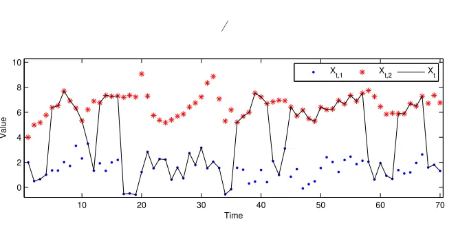
3.2. Independent regimes variant

10 20 30 40 50 60 70 0

2 4 6 8 10

Time

Value

X

t,1 Xt,2 Xt

Fig 2_{. A sample trajectory of the MRS model with independent regimes (black solid line)}

super-imposed on the observable and latent values of the processes in both regimes. The simulation was performed for a model with the following parameters:p11= 0.9,p22= 0.8,α1= 1,β1= 0.7,σ2₁= 1,

γ₁= 0,α₂= 2,β₂= 0.3,σ2

2= 0.01,γ2= 1.

that for the calculation of the conditional pdf (3.1), used in the i) part of the E-step recursions, the information from only one preceding time step is needed. Consequently, the EM algorithm requires storing conditional probabilitiesP(Rt=i|xT) of one time

step only, i.e. 2T values in total.

However, the estimation procedure complicates significantly, if the regimes are independent from each other. Observe, that the values of the mean-reverting regime become latent when the process is in the other state (see Figure2for an illustration). This makes the distribution ofXtdependent on the whole history (x1, x2, ..., xt−1) of the process. As a consequence all possible paths of the state process (R1, R2, ..., Rt)

should be considered in the estimation procedure, implying thatf(xt|Rt=i, Rt−16= i, ..., Rt−j 6= i, Rt−j−1 = i;xt−1;θ(n)) and the whole set of probabilities P(Rt =

it, Rt−1 =it−1, ..., Rt−j = it−j|xt−1;θ(n)) should be used in the E-step. Obviously, this leads to a high computational complexity, as the number of possible state process realizations is equal to 2T _{and increases rapidly with the sample size.}

As a feasible solution to this problemHuisman and de Jong (2002) suggested to use probabilities of the last 10 observations. Apart from the fact that such an ap-proximation still is computationally intensive, it can be used only if the probability of more than 10 consecutive observations from the second regime is negligible.

can be applied with the following approximation of the pdf:

fxt|Rt=i;xt−1;θ(n)

= _√ 1

2πσ_i(n)_|x˜t−1,i|γ

(n)

i · ·exp      −

xt−

1−β_i(n)x˜t−1,i−α(in)

2

2σ_i(n) 2

|x˜t−1,i|2γi(n)

     ,(3.3)

where ˜xt,idenotes the expected value of theith regime at timet, i.e.E Xt,i|xt;θ(n).

Note, that compared to formula (3.1) for the parameter-switching variant, the ob-served value of the processxt−1 is now replaced by the expected value ˜xt−1,i of the

ith regime at timet−1. The following lemma describes how to derive these values.

Lemma 3.2. Expected values E Xt,i|xt;θ(n)

are given by the following recursive formula:

EXt,i|xt;θ(n)

= PRt=i|xt;θ(n)

xt+P

Rt6=i|xt;θ(n)

·

·nα(_in)+1−β(_in)EXt−1,i|xt−1;θ(n)

o

.

It is interesting to note, that

EXt,i|xt;θ(n)

=

t−1

X

k=0 xt−k

1−β(_in)

k

PRt−k=i|xt−k;θ(n)

· · k Y j=1

PRt−j+16=i|xt−j+1;θ(n)

+α(_in)

t−1

X

k=0

1−β(_in)k

k

Y

j=0

PRt−j+16=i|xt−j+1;θ(n)

.

Hence, the expected value E(Xt,i|xt;θ(n)) is a linear combination of the observed

vector x_t and the probabilities P(Rj = i|xj;θ(n)) calculated during the estimation

procedure (see the filtering part of the E-step). This observation shows that using ˜

xt−1,i = E(Xt−1,i|xt−1;θ(n)) in formula (3.3) instead of xt−1, as in formula (3.1) for the parameter-switching variant, the computational complexity of the E-step is greatly reduced.

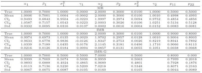
Table 1

Means, 95% confidence intervals (CIl,CIu) and standard deviations (Std) of parameter estimates

obtained from 1000 simulated trajectories of 10000 observations each, for the three studied MRS model types: MR, IMR, and IMR-G.

α1 β1 σ₁2 γ1 α2 β2 σ₂2 γ2 p11 p22 MR

True 1.0000 0.7000 1.0000 0.0000 2.0000 0.3000 0.0100 1.0000 0.5000 0.5000 Mean 1.0006 0.7001 1.0004 -0.0002 2.0000 0.3000 0.0100 1.0010 0.4998 0.4993 CI_l 0.9493 0.6842 0.9504 -0.0223 1.9997 0.2974 0.0094 0.9752 0.4854 0.4856 CIu 1.0587 0.7157 1.0543 0.0223 2.0003 0.3026 0.0106 1.0251 0.5134 0.5128 Std 0.0332 0.0095 0.0316 0.0137 0.0002 0.0016 0.0004 0.0152 0.0083 0.0081

IMR

True 1.0000 0.7000 1.0000 0.0000 2.0000 0.3000 0.0100 1.0000 0.9000 0.8000 Mean 0.9974 0.6973 1.0135 0.0029 1.9702 0.2957 0.0128 1.0010 0.9004 0.8003 CI_l 0.9633 0.6778 0.9836 -0.0126 1.8347 0.2753 0.0026 0.8219 0.8941 0.7892 CIu 1.0339 0.7189 1.0435 0.0176 2.1145 0.3181 0.0496 1.1716 0.9066 0.8113 Std 0.0216 0.0126 0.0184 0.0094 0.0857 0.0131 0.0055 0.1051 0.0038 0.0068

IMR-G

True 1.0000 0.7000 0.5000 0.5000 7.0000 0.5000 0.8000 0.000 Mean 0.9999 0.7009 0.5074 0.5036 6.9959 0.5063 0.7999 0.2018 CI_l 0.9893 0.6888 0.4924 0.4865 6.9689 0.4801 0.7928 0.1876 CIu 1.0113 0.7136 0.5220 0.5209 7.0218 0.5348 0.8071 0.2163 Std 0.0067 0.0075 0.0087 0.0105 0.0160 0.0165 0.0044 0.0089

4. Simulation study

In order to test the performance of the estimation method proposed in Section3.2, we provide a simulation study. For each of the following three MRS model types we generate 1000 sample trajectories:

• MR: with parameter-switching mean-reverting regimes, see (2.3),

• IMR: with independent mean-reverting processes in both regimes, see (2.5), • IMR-G: with a mean-reverting process in the first regime and independent

N(α2, σ22)-distributed random variables in the second regime.

The IMR model is simulated with probabilities of staying in the same regime equal to p11 = 0.9 andp22 = 0.8 for the first and the second regime, respectively. With such a choice of the transition matrix we can expect to see many consecutive observations in each regime. Indeed, the probability of 10 consecutive observations from the first regime is equal to 0.35 and even for 40 consecutive observations that probability is still higher than 0.01. Obviously, such a model cannot be estimated based on the information about only a few prevailing observations.

For each sample trajectory we apply one of the estimation procedures described in Section3. Then, we calculate the means, standard deviations and 95% confidence intervals of the parameter estimates. The values obtained for trajectories consisting of 10000 observations are given in Table 1. All sample means are close to the true parameters with a deviation of no more than 0.03 (in absolute terms). In fact, in most cases the deviation is significantly lower. Moreover, all parameter values are within the obtained 95% confidence intervals. Also the standard deviation of the estimates is quite low and, except forγ2 andα2 in the IMR model, does not exceed 0.04.

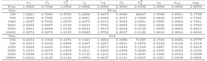
Table 2

Means and standard deviations (Std), over 1000 simulated trajectories, of parameter estimates in the MR model calculated for different sample sizes.

α1 β1 σ2₁ γ1 α2 β2 σ2₂ γ2 p11 p22 True 1.0000 0.7000 1.0000 0.0000 2.0000 0.3000 0.0100 1.0000 0.5000 0.5000

Size Mean

100 0.9904 0.7040 0.8863 0.0455 1.9990 0.3011 0.0088 1.1214 0.4895 0.4962 500 1.0027 0.7000 0.9818 0.0069 2.0000 0.2999 0.0096 1.0201 0.4986 0.4986 1000 1.0034 0.7014 0.9915 0.0021 2.0002 0.3002 0.0097 1.0151 0.4990 0.4989 2000 1.0021 0.7009 0.9966 0.0026 2.0000 0.3000 0.0099 1.0045 0.5002 0.4990 5000 1.0003 0.7003 0.9958 0.0005 2.0000 0.3000 0.0099 1.0035 0.4998 0.5000 10000 1.0006 0.7001 1.0004 -0.0002 2.0000 0.3000 0.0100 1.0010 0.4998 0.4993

Size Std

100 0.3746 0.1111 0.3903 0.2280 0.0279 0.0219 0.0056 0.2797 0.0864 0.0865 500 0.1563 0.0461 0.1535 0.0703 0.0042 0.0077 0.0018 0.0766 0.0350 0.0362 1000 0.1094 0.0311 0.1035 0.0453 0.0020 0.0051 0.0013 0.0518 0.0263 0.0256 2000 0.0719 0.0214 0.0719 0.0298 0.0010 0.0035 0.0008 0.0335 0.0179 0.0180 5000 0.0474 0.0139 0.0455 0.0196 0.0004 0.0023 0.0005 0.0213 0.0115 0.0115 10000 0.0332 0.0095 0.0316 0.0137 0.0002 0.0016 0.0004 0.0152 0.0083 0.0081

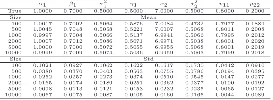
Table 3

Means and standard deviations (Std), over 1000 simulated trajectories, of parameter estimates in the IMR model calculated for different sample sizes.

α1 β1 σ2₁ γ1 α2 β2 σ₂2 γ2 p11 p22 True 1.0000 0.7000 1.0000 0.0000 2.0000 0.3000 0.0100 1.0000 0.9000 0.8000

Size Mean

100 1.0221 0.7280 0.9765 0.0298 2.6473 0.3982 22647 1.0580 0.8951 0.7798 500 1.0002 0.7026 1.0109 0.0061 2.0368 0.3057 0.5569 0.9822 0.8997 0.7956 1000 1.0037 0.7025 1.0070 0.0075 2.0319 0.3052 0.0391 0.9995 0.9004 0.7981 2000 0.9992 0.6987 1.0130 0.0024 1.9781 0.2969 0.0200 1.0046 0.9006 0.7993 5000 1.0001 0.6988 1.0128 0.0044 1.9615 0.2944 0.0139 1.0059 0.9004 0.8001 10000 0.9974 0.6973 1.0135 0.0029 1.9702 0.2957 0.0128 1.0010 0.9004 0.8003

Size Std

100 0.2254 0.1358 0.1975 0.1341 1.3062 0.1986 71587 2.1783 0.0385 0.0779 500 0.0954 0.0558 0.0869 0.0487 0.4207 0.0641 9.0870 0.5930 0.0166 0.0318 1000 0.0668 0.0403 0.0601 0.0312 0.2917 0.0444 0.1958 0.3687 0.0116 0.0218 2000 0.0473 0.0275 0.0408 0.0211 0.2006 0.0306 0.0620 0.2397 0.0083 0.0156 5000 0.0296 0.0176 0.0263 0.0135 0.1213 0.0184 0.0093 0.1606 0.0052 0.0098 10000 0.0216 0.0126 0.0184 0.0094 0.0857 0.0131 0.0055 0.1051 0.0038 0.0068

most cases a sample of 1000 (or even 500 for the MR and IMR-G models) observations yields satisfactory results, as the deviation does not exceed 0.03 (in absolute terms). Especially for the IMR-G model the results are very satisfactory. This is important in view of the fact that a variant of this model is used in Section 5 for modeling electricity spot prices.

5. Application to electricity spot prices

In this study we present how the techniques introduced in Section3can be used to effi-ciently calibrate MRS models to electricity spot prices. We use mean daily (baseload) day-ahead spot prices from the European Energy Exchange (EEX; Germany). The sample totals 1827 daily observations (or 267 full weeks) and covers the 5-year period January 3, 2005 – January 3, 2010.

Table 4

Means and standard deviations (Std), over 1000 simulated trajectories, of parameter estimates in the IMR-G model calculated for different sample sizes.

α1 β1 σ2₁ γ1 α2 σ₂2 p11 p22 True 1.0000 0.7000 0.5000 0.5000 7.0000 0.5000 0.8000 0.2000

Size Mean

100 1.0017 0.7002 0.5064 0.5876 7.0084 0.4732 0.7977 0.1889 500 1.0045 0.7048 0.5058 0.5221 7.0007 0.5068 0.8011 0.2008 1000 0.9997 0.7004 0.5066 0.5137 6.9941 0.5066 0.7995 0.2012 2000 1.0007 0.7012 0.5086 0.5071 6.9971 0.5038 0.8001 0.2020 5000 1.0000 0.7000 0.5072 0.5055 6.9955 0.5068 0.8001 0.2019 10000 0.9999 0.7009 0.5074 0.5036 6.9959 0.5063 0.7999 0.2018

Size Std

100 0.1021 0.0927 0.1062 0.1622 0.1617 0.1730 0.0442 0.0910 500 0.0380 0.0370 0.0403 0.0563 0.0755 0.0786 0.0194 0.0395 1000 0.0252 0.0257 0.0273 0.0374 0.0510 0.0545 0.0147 0.0277 2000 0.0165 0.0174 0.0189 0.0251 0.0362 0.0377 0.0100 0.0192 5000 0.0098 0.0113 0.0121 0.0153 0.0232 0.0235 0.0065 0.0127 10000 0.0067 0.0075 0.0087 0.0105 0.0160 0.0165 0.0044 0.0089

use a single non-parametric long-term seasonal component (LTSC) to represent the long-term non-periodic fuel price levels, the changing climate/consumption conditions throughout the years and strategic bidding practices.

We assume that the electricity spot price,Pt, can be represented by a sum of two

independent parts: a predictable (seasonal) component ft and a stochastic

compo-nent Xt , i.e. Pt = ft+Xt. Further, we let ft be composed of a weekly periodic

part, st, and a LTSC, Tt. The deseasonalization is then conducted in three steps.

First, the long term trendTt is estimated from daily spot pricesPtusing a wavelet

filtering-smoothing technique (for details see Tr¨uck et al.,2007; Weron, 2006). This procedure, also known as low pass filtering, yields a traditional linear smoother. Here we use theS6approximation, which roughly corresponds to bi-monthly (26_{= 64 days)} smoothing.

The price series without the LTSC is obtained by subtracting theS6approximation fromPt. Next, the weekly periodicitystis removed by subtracting the ‘average week’

calculated as the arithmetic mean of prices corresponding to each day of the week (German national holidays are treated as the eight day of the week). Finally, the deseasonalized prices, i.e.Pt−Tt−st, are shifted so that the mean of the new process

is the same as the mean ofPt. The resulting deseasonalized time seriesXt=Pt−Tt−st

can be seen in Figure6.

The second well known feature of electricity prices are the sudden, unexpected price changes, known as spikes or jumps. The ‘spiky’ nature of spot prices is the effect of non-storability of electricity. Electricity to be delivered at a specific hour cannot be substituted for electricity available shortly after or before. Extreme load fluctuations – caused by severe weather conditions often in combination with generation outages or transmission failures – can lead to price spikes. On the other hand, an oversupply – due to a sudden drop in demand and technical limitations of an instant shut-down of a generator – can cause price drops. Further, electricity spot prices are in general regarded to be mean-reverting and exhibit the so called ‘inverse leverage effect’, meaning that the positive shocks increase volatility more than the negative shocks (Knittel and Roberts, 2005).

0 2000 4000 6000 8000 10000 0.5

1 1.5

α1

Sample size

0 2000 4000 6000 8000 10000 0.5

0.6 0.7 0.8 0.9

β1

Sample size

0 2000 4000 6000 8000 10000 0.5

1 1.5

σ

2 1

Sample size

0 2000 4000 6000 8000 10000 −0.2

0 0.2 0.4

γ1

Sample size

0 2000 4000 6000 8000 10000 1.99

2 2.01

α2

Sample size

0 2000 4000 6000 8000 10000 0.28

0.3 0.32 0.34

β2

Sample size

0 2000 4000 6000 8000 10000 0

0.01 0.02

σ

2 2

Sample size

0 2000 4000 6000 8000 10000 0.8

1 1.2 1.4 1.6

γ2

Sample size

0 2000 4000 6000 8000 10000 0.4

0.5 0.6

p11

Sample size

0 2000 4000 6000 8000 10000 0.4

0.5 0.6

p22

Sample size

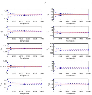
Fig 3_{. 95% confidence intervals of parameter estimates in the MRS model with parameter-switching}

mean-reverting regimes (MR; see Table 1for parameter details). The true parameter values are given by the solid red lines.

three independent states:

Xt=

 



Xt,1 ifRt= 1,

Xt,2 ifRt= 2,

Xt,3 ifRt= 3.

(5.1)

The first (base) regime describes the ‘normal’ price behavior and is given by the mean-reverting, heteroskedastic process of the form:

Xt,1=α1+ (1−β1)Xt−1,1+σ1|Xt−1,1|γ1ǫt, (5.2)

where ǫt is the standard Gaussian noise. The second regime represents the sudden

0 2000 4000 6000 8000 10000 0.8

1 1.2 1.4

α1

Sample size

0 2000 4000 6000 8000 10000 0.4

0.6 0.8 1

β1

Sample size

0 2000 4000 6000 8000 10000 0.8

1 1.2

σ

2 1

Sample size

0 2000 4000 6000 8000 10000 −0.2

0 0.2

γ1

Sample size

0 2000 4000 6000 8000 10000 1

2 3 4 5

α2

Sample size

0 2000 4000 6000 8000 10000 0.2

0.4 0.6 0.8

β2

Sample size

0 2000 4000 6000 8000 10000 0

0.05 0.1 0.15

σ

2 2

Sample size

0 2000 4000 6000 8000 10000 −2

0 2 4

γ2

Sample size

0 2000 4000 6000 8000 10000 0.85

0.9 0.95

p11

Sample size

0 2000 4000 6000 8000 10000 0.7

0.8 0.9

p22

Sample size

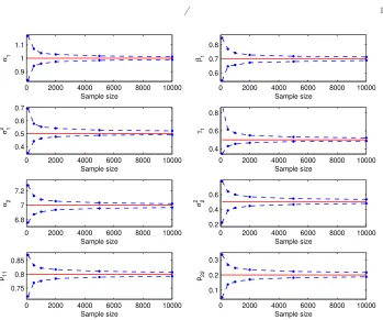
Fig 4_{. 95% confidence intervals of parameter estimates in the MRS model with independent}

mean-reverting regimes (IMR; see Table1for parameter details). The true parameter values are given by the solid red lines.

random variables from the shifted log-normal distribution:

log(Xt,2−X(q2))∼N(α2, σ22), Xt,2> X(q2). (5.3)

Finally, the third regime (responsible for the sudden price drops) is governed by the shifted ‘inverse log-normal’ law:

log(−Xt,3+X(q3))∼N(α3, σ23), Xt,3< X(q3). (5.4)

In the above formulasX(qi) denotes theqi-quantile,qi∈(0,1), of the dataset.

Gener-ally the choice ofqiis arbitrary, however, in this paper we letq2= 0.75 andq3= 0.25,

0 2000 4000 6000 8000 10000 0.9

1 1.1

α1

Sample size

0 2000 4000 6000 8000 10000 0.6

0.7 0.8

β1

Sample size

0 2000 4000 6000 8000 10000 0.4

0.5 0.6 0.7

σ

2 1

Sample size

0 2000 4000 6000 8000 10000 0.4

0.6 0.8

γ1

Sample size

0 2000 4000 6000 8000 10000 6.8

7 7.2

α2

Sample size

0 2000 4000 6000 8000 10000 0.2

0.4 0.6

σ

2 2

Sample size

0 2000 4000 6000 8000 10000 0.75

0.8 0.85

p11

Sample size

0 2000 4000 6000 8000 10000 0.1

0.2 0.3

p22

Sample size

Fig 5_{. 95% confidence intervals of parameter estimates in the MRS model with a mean-reverting}

regime combined with independent Gaussian random variables (IMR-G; see Table1for parameter details). The true parameter values are given by the solid red lines.

dynamics, which implies that the spike (drop) regime distribution should have mass concentrated well above (below) the median.

The deseasonalized prices Xt and the conditional probabilities of being in the

spikeP(Rt= 2|x1, x2, ..., xT) or dropP(Rt= 3|x1, x2, ..., xT) regime for the analyzed

dataset are displayed in Figure6. The prices classified as spikes or drops, i.e. with P(Rt = 2|x1, x2, ..., xT) > 0.5 or P(Rt = 3|x1, x2, ..., xT) > 0.5, are additionally

denoted by dots or ’x’. The estimated model parameters are given in Table5. The obtained base regime parameters are consistent with the well known properties of electricity prices. Positive γ is responsible for the ‘inverse leverage effect’, while β= 0.42 indicates a high speed of mean-reversion. Considering probabilities of staying in the same regime pii we obtain quite high values for each of the regimes, ranging

from 0.65 for the spike regime up to 0.96 for the base regime. As a consequence, on average there are many consecutive observations from the same regime.

-0 200 400 600 800 1000 1200 1400 1600 1800 0

50 100 150 200 250 300

EEX price [EUR/MWh]

Base Spike Drop

0 200 400 600 800 1000 1200 1400 1600 1800 0

0.5 1

P(S)

0 200 400 600 800 1000 1200 1400 1600 1800 0

0.5 1

P(D)

Days [January 3, 2005 − January 3, 2010]

Fig 6_{. Calibration results of the MRS model with three independent regimes fitted to the}

desea-sonalized EEX prices. The lower panels display the conditional probabilities P(S) = P(Rt =

2|x₁, x₂, ..., xT) and P(D) = P(Rt = 3|x₁, x₂, ..., xT) of being in the spike or drop regime,

re-spectively. The prices classified as spikes or drops, i.e. withP(S)>0.5orP(D)>0.5, are denoted by dots or ’x’ in the upper panel.

values of a Kolmogorov-Smirnov (K-S) goodness-of-fit type test for each of the individ-ual regimes, as well as, for the whole model (for test details seeJanczura and Weron, 2010). The goodness-of-fit results are summarized in Table6. Observe that almost all differences between the data and the model-implied statistics are less than 1%, the only exception is the variance, but still the value of 2.38% indicates quite a good fit. Moreover, all K-S test p-values are higher than the commonly used 5% significance level, so we cannot reject the hypothesis that the dataset follows the 3-regime MRS model.

6. Conclusions

In this paper we have proposed a method that greatly reduces the computational burden induced by the introduction of independent regimes in MRS models. Instead of storing conditional probabilities for each of the possible state process paths, i.e. 2T

Table 5

Calibration results of the MRS model with three independent regimes fitted to the deseasonalized EEX prices

Parameters Probabilities

α1 β1 σ2₁ γ1 α2 σ₂2 α3 σ2₃ p11 p22 p33 19.98 0.42 0.15 0.70 2.65 1.03 2.41 0.35 0.9587 0.6500 0.7778

Table 6

Goodness-of-fit statistics for the 3-regime MRS model fitted to the deseasonalized EEX prices. For moments and quantiles the relative differences between the sample and the model implied statistics

are given (the latter are obtained from 1000 simulations).

Moments Quantiles K-S test p-values E(X) Var(X) 0.1 0.25 0.5 0.75 0.9 Base Spike Drop Model -0.05% -2.38% 0.36% 0.05% -0.01% -0.18% -0.40% 0.82 0.08 0.40 0.35

i.e. 2T values. We have performed a limited simulation study to test the efficiency of the new method and applied it to a sample series of electricity spot prices.

The simulation study has shown that all sample means are close to the true pa-rameter values (and all true papa-rameter values are within the obtained 95% confidence intervals). Moreover, the standard deviations, as well as, the width of the confidence intervals decrease with increasing sample size. Looking at the means, in most cases a sample of 1000 (or even 500 for the MR and IMR-G models; for model acronyms and definitions see Section 4) observations yields satisfactory results, as the devia-tion does not exceed 0.03 (in absolute terms). Especially for the IMR-G model the results are very satisfactory. This is important in view of the fact that variants of this model are popular in the energy finance literature. In particular, a model of this type (with shifted log-normal spike and price drop regimes independent from the base mean-reverting regime) is calibrated in Section5to a sample series of deseasonalized wholesale electricity spot prices from the German EEX market.

The proposed MRS model fits market data well and also contains unique features that allow for useful interpretations of the price dynamics. In particular, the parameter γcan be treated as a parameter representing the ‘degree of inverse leverage’. A positive value (e.g. γ1 = 0.70 as in Table 5) indicates ‘inverse leverage’. Recall, that the ‘inverse leverage effect’ reflects the observation that positive electricity price shocks increase volatility more than negative shocks.Knittel and Roberts(2005) attributed this phenomenon to the fact that a positive shock to electricity prices can be treated as an unexpected positive demand shock. Therefore, as a result of convex marginal costs, positive demand shocks have a larger impact on price changes relative to negative shocks.

Appendix

Proof of Lemma3.1. Observe that the joint density f(x1, x2, ..., xT) can be written

as a product of appropriate conditional densities

f(xT|xT−1, xT−2, ..., x1)f(xT−1|xT−2, xT−3, ..., x1). . . f(x2|x1)f(x1). (6.1)

Moreover,Xtconditional onxt−1, xt−2, ..., x1 has a Gaussian distribution with mean (1−βi)xt−1+αi and standard deviationσi2|xt−1|γi. Thus, theith regime weighted log-likelihood function is given by the following formula:

ln[L(αi, βi, σi, γi)] = − T

X

t=2

P(Rt=i|xT;θ(n))·

·

"

ln√2πσi|xt−1|γi

+(xt−(1−βi)xt−1−αi) 2

2σ2_i|xt−1|2γi

#

. (6.2)

Note, that the parameter vectorθ(n)is omitted in what follows to simplify the nota-tion. In order to find the maximum likelihood (ML) estimates, the partial derivatives of ln(L) are set to zero. This leads to the following system of equations:

T

X

t=2

P(Rt=i|xT)|xt−1|−2γi(xt−(1−βi)xt−1−αi) = 0,

T

X

t=2

P(Rt=i|xT)xt−1|xt−1|2γi(xt−(1−βi)xt−1−αi) = 0,

T

X

t=2

P(Rt=i|xT)|xt−1|−2γi(xt−(1−βi)xt−1−αi)2=

=σ2_i

T

X

t=2

P(Rt=i|xT),

T

X

t=2

P(Rt=i|xT)|xt−1|−2γiln|xt−1|(xt−(1−βi)xt−1−αi)2=

=σ2_i

T

X

t=2

Now, the ML estimates forαi,βi, and σi2can be explicitly derived:

ˆ αi =

T

P

t=2

P(Rt=i|xT)|xt−1|−2γi(xt−(1−βˆi)xt−1)

T

P

t=2

P(Rt=i|xT)|xt−1|−2γi

,

ˆ βi =

T

P

t=2

P(Rt=i|xT)xt−1|xt−1|−2γiB1

T

P

t=2

P(Rt=i|xT)xt−1|xt−1|−2γiB2 ,

B1=xt−xt−1−

PT

t=2P(Rt=i|xT)|xt−1|−2γi(xt−xt−1)

PT

t=2P(Rt=i|xT)|xt−1|−2γi ,

B2=

PT

t=2P(Rt=i|xT;θ(n))xt−1|xt−1|−2γi

PT

t=2P(Rt=i|xT)|xt−1|−2γi − xt−1,

ˆ σ2 i = T P t=2

P(Rt=i|xT)|xt−1|−2γi(xt−αˆi−(1−βˆi)xt−1)2

T

P

t=2

P(Rt=i|xT)

,

while the estimate forγi has to be approximated numerically (due to the entangled

form of the derivatives of the log-likelihood function (6.2)).

Proof of Lemma3.2. LetX_t= (X1, X2, ..., Xt). Observe that

Xt,i=IRt=iXt+IRt6=i[αi+ (1−βi)Xt−1,i+σi|Xt−1,i|

γi_ǫ

t], (6.3)

whereIxis the indicator function. Taking the expected value conditional onXtyields:

EXt,i|Xt;θ(n)

= PRt=i|Xt;θ(n)

Xt+P

Rt6=i|Xt;θ(n)

h

α(_in)+

+1−β(_in)EXt−1,i|Xt, Rt6=i;θ(n)

+

+σ_i(n)E_|Xt−1,i|γ

(n)

i ǫ

t|Xt, Rt6=i;θ(n)

i

.

SinceXt−1,i and ǫt are independent of theσ-algebra generated by{Xt, Rt 6=i} we

have

E|Xt−1,i|γ

(n)

i _ǫ

t|Xt, Rt6=i;θ(n)

=E|Xt−1,i|γ

(n)

i _ǫ

t|Xt−1;θ(n)

,

and

EXt−1,i|Xt, Rt6=i;θ(n)

=EXt−1,i|Xt−1;θ(n)

.

expected values:

E_|Xt−1,i|γ

(n)

i ǫ

t|Xt−1;θ(n)

=

=EhE_|Xt−1,i|γ

(n)

i ǫ

t|Xt−1, Xt−1,i;θ(n)

|X_t−1;θ(n)

i

=

=Eh_|Xt−1,i|γ

(n)

i E

ǫt|Xt−1, Xt−1,i;θ(n)

|X_t−1;θ(n)

i

=

=Eh|Xt−1,i|γ

(n)

i E(ǫ

t)|Xt−1;θ(n)

i

= 0,

which implies

EXt,i|Xt;θ(n)

= P(Rt=i|Xt;θ(n))Xt+P(Rt6=i|Xt;θ(n))·

·hα(_in)+ (1−β_i(n))EXt−1,j|Xt−1;θ(n)

i

.

Finally, substituting the variablesX_twith their observationsx_tcompletes the proof.

References

Barz, G., Johnson, B. (1998). Modeling the prices of commodities that are costly to store: The case of electricity. Proceedings of the Chicago Risk Management Conference.

Benth, F.E., Benth, J.S., Koekebakker, S. (2008). Stochastic Modeling of Electricity and Related Markets. World Scientific, Singapore.

Cappe, O., Moulines E., Ryden T. (2005). Inference in Hidden Markov Models. Springer.

Christensen, T., Hurn, S., Lindsay, K. (2009). It never rains but it pours: modeling the persistence of spikes in electricity prices. The Energy Journal 30(1), 25-48. Cox, J.C., Ingersoll, J.E., Ross, S.A. (1985). A theory of the term structure of interest

rates. Econometrica 53, 385-407.

De Jong, C. (2006). The nature of power spikes: A regime-switch approach. Studies in Nonlinear Dynamics & Econometrics 10(3), Article 3.

Dempster, A., Laird, N., Rubin, D.B. (1977). Maximum likelihood from incomplete data via the EM algorithm. Journal of the Royal Statistical Society 39, 1-38. Deng, S.-J. (1998). Stochastic models of energy commodity prices and their

applica-tions: Mean-reversion with jumps and spikes. PSerc Working Paper 98-28.

Ethier, R., Mount, T., (1998). Estimating the volatility of spot prices in restructured electricity markets and the implications for option values. PSerc Working Paper 98-31.

Fink, G.A. (2008). Markov Models for Pattern Recognition: From Theory to Appli-cations. Springer.

Franses, P.H., van Dijk, D. (2000). Nonlinear Time Series Models in Empirical Fi-nance. Cambridge University Press.

Hamilton, J. (1989). A new approach to the economic analysis of nonstationary time series and the business cycle. Econometrica 57, 357-384.

Hamilton, J. (1990). Analysis of time series subject to changes in regime. Journal of Econometrics 45, 39-70.

Huisman, R. (2009). An Introduction to Models for the Energy Markets. Risk Books. Huisman, R., de Jong, C. (2002). Option formulas for mean-reverting power prices

with spikes. ERIM Report Series Reference No. ERS-2002-96-F&A.

Janczura, J., Weron, R. (2010). An empirical comparison of alternate regime-switching models for electricity spot prices. Energy Economics 32, 1059-1073.

Janczura, J., Weron, R. (2010). Goodness-of-fit testing for regime-switching models. Working paper. Available at MPRA: http://mpra.ub.uni-muenchen.de/22871. Kaminski, V. (1997). The challenge of pricing and risk managing electricity

deriva-tives. In: The US Power Market. Risk Books.

Karakatsani, N.V., Bunn, D.W. (2008). Intra-day and regime-switching dynamics in electricity price formation. Energy Economics 30, 1776-1797.

Kim, C.-J. (1994). Dynamic linear models with Markov-switching. J. Econometrics 60, 1-22.

Knittel, C.R., Roberts, M.R. (2005). An empirical examination of restructured elec-tricity prices. Energy Economics 27, 791-817.

Mamon, R.S., Elliott, R.J., eds. (2007). Hidden Markov Models in Finance. Interna-tional Series in Operations Research & Management Science, Vol. 104, Springer. Mount, T.D., Ning, Y., Cai, X. (2006). Predicting price spikes in electricity markets

using a regime-switching model with time-varying parameters. Energy Economics 28: 62-80.

Scharpf, R.B., Parmigiani, G., Pevsner, J., Ruczinski, I. (2008) Hidden Markov models for the assessment of chromosomal alterations using high-throughput SNP arrays. The Annals of Applied Statistics 2(2), 687-713.

Shirley, K.E., Small, D.S., Lynch, K.G., Maisto, S.A., Oslin, D.W. (2010). Hidden Markov models for alcoholism treatment trial data. The Annals of Applied Statistics 4(1), 366-395.

Tr¨uck, S., Weron, R., Wolff, R. (2007). Outlier treatment and robust approaches for modeling electricity spot prices. Proceedings of the 56th Session of the ISI. Available at MPRA: http://mpra.ub.uni-muenchen.de/4711/.

Vasicek, O. (1977). An equilibrium characterization of the term structure. Journal of Financial Economics 5, 177-188.

Weron, R. (2006). Modeling and forecasting electricity loads and prices: A statistical approach. Wiley, Chichester.