Application of Scheffe's Theory to Develop Mathematical Prediction Model to Predict UCS for Hybrid Containing Organic Soil and POFA OPC Additives

Application of Scheffe's Theory to Develop

Mathematical Prediction Model to Predict UCS for

Hybrid Containing Organic Soil and

POFA-OPC Additives

Yaser Gamil

*

_{, Kemas Ahmed Zamahri, Ismail Bakar}

Faculty of Civil and Environmental Engineering, Tun Hussein Onn University of Malaysia, Malaysia

Copyright©2018 by authors, all rights reserved. Authors agree that this article remains permanently open access under the terms of the Creative Commons Attribution License 4.0 International License

Abstract

Unconfined compressive strength (UCS) is very significant parameters to evaluate the strength property of soil. In laboratory, it requires machinery and effort to determine UCS. Therefore, to predict UCS of organic soil stabilized by Palm Oil Fuel Ash-Ordinary Portland Cement (POFA-OPC) at less time and less cost for additive selection percentage the prediction model can simplify the selection of additives percentage by reducing the random selection of additives percentage and its disadvantageous results. As a result of that, the use of the prediction model eliminates the arbitrary selection of design mixes and its associated disadvantages. This paper is a continuous to previous publication by authors on the application of Scheffe’s theory to predict resilient modulus however, this paper focused on the implementation of Scheffe’s regression theory to develop mathematical model to predict UCS based on proposed mix proportions. The mixes were developed analytically from previous adopted rations of additives. The materials were characterized and investigated for the primary properties then the samples of POFA –OPC additives were prepared for the size of 70mm diameter and 140 height. 25 samples were designed and characterized for each mix proportion based on the UCS in 28 days curing. The Results of observed values from laboratory analysis are used to develop the mathematical model. In addition to that, the model was statistically scrutinized and confirmed for the adequacy and validity using f-test. The results showed that, the model is verified and adequate to predict UCS for any random POFA-OPC additives percentage.

Keyword

s

Palm Oil Fuel Ash, Unconfined Compressive Strength, Mathematical Prediction Model

1. Introduction

Mathematical prediction models are very crucial in the area of civil engineering especially in laboratory works because they help minimize time and cost to find the properties of mixes and determine the optimum amount of additives. In the area of soil modification with by-products, it is necessary to decide the percentage of additives that could provide better soil properties. [1]. Unconfined Compressive strength (UCS) is significant parameter to judge the strength and resistance of soil to lateral and vertical loads. In order to obtain the UCS for any hybrid it requires enormous effort and machinery. Several prediction and optimization mathematical polynomials have emerged in the applications of concrete and soil stabilizations to do away with these issues. Of these polynomial regression models, Scheffe [2] has developed a polynomial equation to be used for optimization to find the optimum content of any factor or materials in additives for experiments with different mixes based on regression theory.

Scheff’s [2] equation has been implemented in the prediction of UCS for concrete but not in soil property modification. According to study by Mbadike and Osadeb [3], the equation was used to determine the optimum value of UCS in concrete. In addition to that Onwuka et al. [4], has used Scheffe’s theory to predict the mix ratios for most economical and durable concrete. In another study by Okere et al. [5], it was implemented to determine the optimum concrete cost. Gamil & Bakar [6] have implemented Scheffe’s theory to predict Resilient Modulus for mixes used in road construction.

expansion. One of these results is the huge amount of waste generated from palm oil mills. Palm Oil Fuel Ash (POFA) is considered one of the major effluents which are normally discharged to particular landfills. POFA has been to show significant chemicals and is a major pollutant to soil.

In Term of statistics, palm oil accounts for 20% and 46% of the global oil and fats production trade respectively [7]. Malaysia is considered as the second largest producer and trading exporter of palm oil with approximate amount of 50% of the world share production and 61% of exports [8]. The expansion of oil palm plantings in Malaysia during the past 41 years has been phenomenal and remarkable [7]. From a mere 55000 hectares in 1960, the oil palm planted area had expanded to 3.5 million hectares by 2001, occupying 60% of the agricultural land in the country. The rapid expansion in oil palm cultivation resulted in a corresponding increase in palm oil production from less than 100,000 tons in 1960 to 11.8 million tons in 2001. In 2005, the total area of palm cultivation was 4 million hectares [7]. According to the European report of palm oil statistics [9], the oil palm plantation area in Malaysia reached 5 million hectares an increase of 3.0% from 4.85 million hectares in 2011.

In spite of all the advantages of palm oil, there are many disadvantages resulted from palm oil industries which include the huge amount of waste generated from the process of oil production. The waste generated from oil production can have several forms and types based on the level of temperature implied and POFA is an ash generated in the mill in the form of dust or ash. This waste can be used as stabilization additives and fills for soil [10].

In many studies POFA is considered as by-product materials generated from palm oil mills and may have negative impact to the environment if disposed in landfills [11]. The process of its production is initially from the burning of oil shells in the boiler of factories [12]. It is approximated that, 5% of the waste is considered for POFA [13]. It was stated that, in every 100 tons of fresh oil fruit, approximately 7 tons of fiber are produced and 20 tons of nut shells are generated. In Malaysia 60 million of tons the total solid wastes were generated annually [14]. This large quantity creates huge problem of disposal [15]. In many countries POFA is dumped into landfills without any profitable returns [16]. The environment has been affected due to the expansion of landfills to accommodate the tremendous amount of POFA disposal [17]. Therefore, it attracted researchers to study its properties and positive

returns toward using in concrete and soil stabilizations to replace raw materials such as OPC and fillers [18].

POFA has been used in many applications in construction and soil stabilization. It was proven that, POFA exhibit as Pozzolanic materials in which it can be used as binder or filler in concrete [13, 19, 20].Likewise, POFA contains high percentage of silica oxide which can react with calcium hydroxide (Ca(OH)2) generated from

the hydration process; and the pozzolanic reactions produce more calcium silicate hydrate (C-S-H) gel compound as well as reducing the amount of calcium hydroxide [21, 22]. It was demonstrated by Phani Kumar et al. [23], POFA can reduce plasticity of expansive soil and the free swelling index has been reduced by the addition of POFA. In addition to that, POFA was used to stabilize sot soil such as clayey soil and reduced the plasticity index of clay, decreased the moisture content, increased the dry density of clay and also increased the UCS [24].

Organic soil is a type of soil that contains organic matters and mostly exists in nature due to the decomposition of plants and animals overtime [25].Farnham et al.[26], described organic soil as fibrous or amorphous according. It is an acidic and usually has pH value less than 5 in addition to that, it possesses low bulk density, low bearing capacity of strength and higher water contents [27]. It is also prescribed as expansive soil [28]. Organic soils accommodate large areas around the world and replacing it with other type of soil can cost higher and yield to negative impact to the environment. Therefore, it requires more treatments to modify its initial properties to be used as construction materials. This study is focused on the stabilization of organic planation soil stabilized with POFA and OPC. In addition to that, the mathematical prediction model will be used to predict the UCS and the percentage of additives required to achieve certain strength of stabilized soil. The developed mix is aimed to be used in road construction.

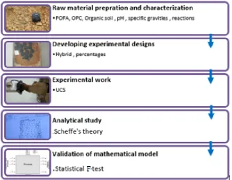
2. Study Methodology

Figure 1. Methodological Study Process Materials used in this study are collected from different

sites in Malaysia. POFA was collected from Kluang in the state of Johor. Laterite gravel was collected from Bukit Nanning quarry in Muar. The organic soil was collected from Ulu Tiram, Johor Bahru where the site is nearby newly constructed road in the form of disturbed samples’ in this study has been treated by heating it for an hour under 500o_{C to remove the access carbon which may}

results negatively in the reactivity analysis.

The experimental work was carried out in accordance to standards and term of references. The samples were prepared in the laboratory and cured for 28 days and examined for UCS. The standard procedures are based on ASTM D2166 / D2166M - 13 Standard Test Method for Unconfined Compressive Strength [29]. The sample size is 70mm diameter and height of 140mm. The total number of sample was 25 in which prepared using similar compaction energy.

3. Experimental and Analytical Design

Experimental design is used to develop hybrid of different parameters. In this study, the main materials are POFA, organic soil, laterite gravel and water. The percentages of each material are described in this section. However, analytical design is used to imply Scheffe's techniques to develop the proportions of experimental mixes.

Prior to that, to embrace the utilization of Scheffe's techniques in enhancement display. A simplex grid is produced to be as basic portrayal of lines joining the

particles of blend which is compelled with the hypothetical findings which implies the qualities must be inside the variable space for a trial and outside the component space for confirmations of the created indication. Consequently, the particles are constituent segments of the blend. The constituent components of this model are POFA, Soil, Laterite rock and OPC. In any case, it gives a simplex of a blend of four segments. However, the simplex cross section of these four parts blend is three-dimensional strong equilateral tetrahedron. In a condition of Scheffe’s method [2], the components are subjected to the constraint that the sum of all the components must be equal to “one” which means:

𝑥𝑥1+𝑥𝑥2+ 𝑥𝑥3+ 𝑥𝑥4+⋯… … . .𝑥𝑥𝑞𝑞 (1) ∑ 𝑥𝑥𝑞𝑞𝑖𝑖 𝑖𝑖= 1 (2)

Where:

“q” is the number of components of mixture

“Xi” is the proportion of the ith _{components in the}

mixture which elaborates the weights in this context. It is important to do a change from real to pseudo segments real blend to build up the model since the total of the blend part should be one. Hence, the actual components represent the proportion of the ingredients based in the theoretical constraints while the pseudo components represent the proportion of the components of the ith _{components in the mixture i.e. X}

1, X2, X3, X4. In

any case, it must consider the four-part blend tetrahedron simplex cross section, let the vertices of this tetrahedron (foremost arranges) be depicted by A1, A2, A3, A4.

[image:3.595.133.468.83.343.2]

previous practicing manual and literatures which are arranged for the vertices of the tetrahedron in Fig. 2. The developed mixes are a 4*4 matrix which can be developed to experimentally design the mixes.

Ai :( POFA: Soil: Laterite Gravel: Cement); {A1 :( 0.04:

1: 0.1: 0.04)}, {A2 :( 0.024: 1: 0.15: 0.036)}, {A3 :( 0.012:

1: 0.2: 0.028)}, {A4 :( 0.004: 1: 0.3: 0.016)}

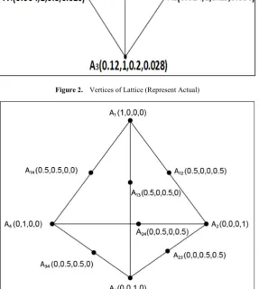
Figure 2 shows a vertices that represents the actual proportions of mix design which was developed based on previous literatures but if the mix is summed up the results will be more than 1 which doesn’t satisfy Scheffe’s condition therefore to make a pseudo representation figure 3 is developed to represent the actual mixes in which the summation is equals one then Scheffe’s theory condition is fulfilled.

To precede the analytical procedure let X denotes the pseudo components and Z denotes actual components then,

for the processes of converting pseudo to actual use the following equations by Scheffe’s:

[𝒁𝒁] = [𝑨𝑨𝑨𝑨] (3) Where, A is a matrix whose components are of arbitrary mix proportions. Then to find “A” Z and X must be known then “A” is the inverse of the matrix.

“X” is selected from the pseudo representations in Figure 3, “Z” represent the matrix in Figure 2.

Then, by expanding equations (3) the actual components of Z will be determined respectively. Table 1 shows the corresponding values of pseudo and actual. Where Yi represents the developed matrices from the

pseudo and actual lattices however Ci represents the

Control Points Calculated within the factor space and Cij

represents Control points calculated outside the factor space.

[image:4.595.155.442.299.482.2]

Figure 2. Vertices of Lattice (Represent Actual)

[image:4.595.156.444.397.718.2]

Table 1. Pseudo Component with Corresponding Actual Component Values Where: Actual (Zi) and Pseudo (Xi) components

No of mix X1 X2 X3 X4 Response Z1 Z2 Z3 Z4

1 1 0 0 0 Y1 0.04 1 0.1 0.04

2 0 1 0 0 Y2 0.024 1 0.15 0.036

3 0 0 1 0 Y3 0.012 1 0.2 0.028

4 0 0 0 1 Y4 0.004 1 0.3 0.016

5 0.5 0.5 0 0 Y12 0.032 1 0.125 0.038

6 0.5 0 0.5 0 Y13 0.026 1 0.15 0.034

7 0.5 0 0 0.5 Y14 0.022 1 0.2 0.028

8 0 0.5 0.5 0 Y23 0.018 1 0.175 0.032

9 0 0.5 0 0.5 Y24 0.014 1 0.225 0.026

10 0 0 0.5 0.5 Y34 0.008 1 0.25 0.022

Control Points Calculated within the factor space

11 0.5 0.25 0.25 0 C1 0.029 1 0.1375 0.036

12 0.25 0.25 0.25 0.25 C2 0.02 1 0.1875 0.03

13 0 0.25 0.25 0.5 C3 0.011 1 0.2375 0.024

14 0 0.25 0 0.75 C4 0.009 1 0.2625 0.021

15 0.75 0 0.25 0 C5 0.033 1 0.125 0.037

16 0 0.5 0.25 0.25 C6 0.016 1 0.2 0.029

17 0.25 0 0.5 0.25 C7 0.017 1 0.2 0.028

18 0.75 0.25 0 0 C8 0.036 1 0.1125 0.039

19 0 0.75 0.25 0 C9 0.021 1 0.1625 0.034

20 0 0.4 0.4 0.2 C10 0.0152 1 0.2 0.03

Control points Calculated outside the factor space

21 0.5 0.5 0.5 0.5 C11 0.016 1 0.2 0.027

22 0.25 0 0.25 0.5 C12 0.015 1 0.225 0.025

23 0.5 0 0.5 0 C13 0.026 1 0.15 0.034

24 0.25 0.25 0.25 0 C14 0.019 0.75 0.1125 0.026

25 0 0.5 0.5 0.25 C15 0.019 1.25 0.25 0.036

4. Results and Analysis

This section introduces the results of developing prediction model to predict UCS of the hybrid.

4.1. Materials Characterization

In order to determine the effect of POFA which is used in this study on the soil reactivity, the chemical compositions are determined in figure 4.

Figure 4. Chemical Compositions for Treated, Untreated POFA and OPC

Figure 4 illustrates the chemical composition of POFA

in both forms treated and untreated. It is shown that POFA exhibit high percentage of Cao and SiO2 which is

considered pozzolan materials and possess high potential to be partial cement replacement. The large amount of silica contributes to the cementation process when mixing with binder such as cement. It shows the possibility of modifying the property of POFA by removing the excessive amount of carbons and unwanted constituents. By referring to ASTM C-618 standard[31], it shows the used POFA is classified as class C because the amount of SiO2 content is between 50%-70% hence it is also

described in the relevant standard that Class C most useful in “performance” mixes, pre-stressed applications, and other situations where higher early strengths are important. Moreover, it is useful in soil stabilization.

4.2. Effect of POFA to Soil Density

[image:5.595.56.540.90.462.2]

Series of density tests were conducted to determine the initial percentage of POFA content in the proposed mix.

[image:5.595.60.295.588.711.2]

15% however it started to drop if the percentage more than 15%. The increment of POFA after the density reached its optimum causes drop of density because the mass decreased and the bulk density decreased too.

Figure 5. POFA Content vs. Dry density

4.3. Sieve Analysis for the Soil

In this part both wet and dry sieving were carried out to determine the gradation of soil in order to check its average particle size.

Table 2. Wet sieving Results

Opening size (mm) Mass retained (g)

0.425 329.9

0.075 213.6

Lost in washing over 0.075mm 156.5

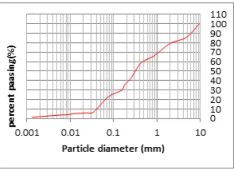
[image:6.595.54.545.115.279.2]

However, using particle less than 0.075 to conduct the hydrometer test based on the sedimentation process with the reference of ASTM (C136-96a) Standard Test Method for Particle-Size Analysis of Soils. The results are shown in figure 6 which was basically calculated based on sieve 200 passing which is taken from sieve analysis data.

Figure 6. Combined Sieve Analysis and Hydrometer Analysis Curves for Soil

4.4. Summary of Soil Properties

Table 3. Summary of Property Indexes for Natural Soil

Properties Results

Atterberg limit LL =30.21%., Pl=23.15%, PI=7.06%

Grain size distribution

Aperture size (mm) Percentage finer (%)

≥9.50 100

4.75 85.73

0.075 23

Particle Density 2.648

pH 6.8 pH

Average moisture content 16%

OMC 9.47%

Maximum dry density 18.55 KN/m3

Table 3 presents the primary properties indexes for the soil, it is shown that the soil pH scale is nearly to be neutral but less than 7 in the scale of acid hence it is not considered acidic. Based on the past technical report developed by US army [32], it is shown that for the soil to be reactive pH scale has to be about 12.4 however to increase the pH of natural soil then lime or cement has to be added to make the soil react with the additives in order to be microstructural reacting to improve its property in term of strength and stiffness. The soil contains organics because it was collected from plantation area of palm oil. In term of Atterberg limit, the soil has small plasticity index which refers lower water absorbent capacity, and thus the quantity and quality of clay minerals can be characterized indirectly and the soil is considered less cohesive. The average moisture content was recorded after the soil was excavated from the site and the OMC with dry density were conducted in the laboratory.

4.5. Development of Mathematical Model

Scheffe (1985) has developed polynomial equation to be used for laboratory optimization models. In this study, it is used to develop prediction model for UCS. The following is the polynomial equation developed by Scheffe (1985):

𝑌𝑌=𝛼𝛼1𝑧𝑧1+𝛼𝛼2𝑧𝑧2+𝛼𝛼3𝑧𝑧3+𝛼𝛼4𝑧𝑧4+𝛼𝛼12𝑧𝑧1𝑧𝑧2+𝛼𝛼13𝑧𝑧1𝑧𝑧3+ 𝛼𝛼14𝑧𝑧1𝑧𝑧4+𝛼𝛼23𝑧𝑧2𝑧𝑧3+𝛼𝛼24𝑧𝑧2𝑧𝑧4+𝛼𝛼34𝑧𝑧3𝑧𝑧4 (4)

In which: 𝛼𝛼𝑖𝑖 and 𝛼𝛼𝑖𝑖𝑗𝑗 are coefficients and Z𝑖𝑖 are the

pseudo components of blend. The Y function is the response function at any point of observation, Zi is the predictor and αi is the coefficient of the prediction model

equations.

[image:6.595.54.295.392.453.2] [image:6.595.58.295.535.706.2]

4.6. Determination of Prediction Model Coefficients

To determine the standard coefficient of the model in equation 4, the responses has to be observed for the first ten mixes where Y(n) _{correspond to Zi}(n) _{equation 4 can be}

written in the following form:

𝑌𝑌(𝑛𝑛)_{=∑ 𝛼𝛼}

𝑖𝑖𝑧𝑧𝑖𝑖(𝑛𝑛)+∑ 𝛼𝛼𝑖𝑖𝑖𝑖𝑧𝑧𝑖𝑖(𝑛𝑛) 𝑧𝑧𝑖𝑖(𝑛𝑛) (5)

Where 1 ≤ I ≤ j ≤ 4 and n = 1, 2, 3, …….,10. Equation (5) can be altered in the form of matrix

�𝑌𝑌(𝑛𝑛)_{�=�𝑍𝑍}(𝑛𝑛)_{�{𝛼𝛼} (6)}

By restructuring equation (6) then results the following equation:

{𝛼𝛼} =�𝑍𝑍(𝑛𝑛)_�−1_�𝑌𝑌(𝑛𝑛)_{� (8)}

Then, allowing the actual mixes in table 1 be represented by Zi(n) _{and the corresponding fractional}

portions, Zif(n) _{are presented in Table 4.}

Table 4 demonstrates the actual mixes which were developed based on Scheffe simplex lattice and the corresponding fractional values which is used to continue the mathematical calculations to determine the coefficients in the mathematical prediction model these values of the fractional portions Z(n) _{were used to develop}

Z(n) _{matrix and the inverse of Z}(n) _{matrix. The values of}

Y(n) _{matrix are determined from laboratory tests from}

resilient modulus and unconfined compressive strength. With the values of the matrices Y(n) _{and Z}(n) _{known, it is}

easy to determine the values of the constant coefficients of equation (5).

Table 4. Actual Mix Proportions and Their Corresponding Fractional values

Mix No Z1 Z2 Z3 Z4 Total of Si Response Z1f Z2f Z3f Z4f

1 0.04 1 0.1 0.04 1.18 Y1 3.390 84.746 8.475 3.390

2 0.024 1 0.15 0.036 1.21 Y2 1.983 82.645 12.397 2.975

3 0.012 1 0.2 0.028 1.24 Y3 0.968 80.645 16.129 2.258

4 0.004 1 0.3 0.016 1.32 Y4 0.303 75.758 22.727 1.212

5 0.032 1 0.125 0.038 1.195 Y12 2.678 83.682 10.460 3.180

6 0.026 1 0.15 0.034 1.21 Y13 2.149 82.645 12.397 2.810

7 0.022 1 0.2 0.028 1.250 Y14 1.760 80.00 16.00 2.240

8 0.018 1 0.175 0.032 1.225 Y23 1.469 81.633 14.286 2.612

9 0.014 1 0.225 0.026 1.265 Y24 1.107 79.051 17.787 2.055

10 0.008 1 0.25 0.022 1.280 Y34 0.625 78.125 19.531 1.719

11 0.029 1 0.1373 0.036 1.202 C1 2.413 83.195 11.423 2.995

12 0.02 1 0.1875 0.03 1.238 C2 1.616 80.775 15.145 2.423

13 0.011 1 0.2375 0.024 1.273 C3 0.864 78.555 18.657 1.885

14 0.009 1 0.2625 0.021 1.293 C4 0.696 77.340 20.302 1.624

15 0.033 1 0.125 0.037 1.195 C5 2.762 83.682 10.460 3.096

16 0.016 1 0.2 0.029 1.245 C6 1.285 80.321 16.064 2.329

17 0.017 1 0.2 0.028 1.245 C7 1.364 80.257 16.051 2.247

18 0.036 1 0.1125 0.039 1.188 C8 3.030 84.175 9.470 3.283

19 0.021 1 0.1625 0.034 1.218 C9 1.724 82.102 13.342 2.791

20 0.0152 1 0.2 0.0288 1.244 C10 1.222 80.386 16.077 2.315

21 0.016 1 0.2 0.027 1.24 C11 1.20 80.41 16.10 2.28

22 0.015 1 0.225 0.025 1.265 C12 1.186 79.051 17.787 1.976

23 0.026 1 0.15 0.034 1.210 C13 2.149 82.645 12.397 2.810

24 0.019 0.75 0.1125 0.026 0.908 C14 2.093 82.599 12.390 2.863

[image:7.595.59.541.296.610.2]

Table 5. The determination of Z n _{matrix values based on table 2}

No Z1 Z2 Z3 Z4 Z1Z2 Z1Z3 Z1Z4 Z2Z3 Z2Z4 Z3Z4 UCS response _kPa

1 3.4 84.70 8.50 3.40 288.0 28.9 11.60 720.0 288.0 28.90 1394.3

2 2.0 82.60 12.40 3.00 165.2 24.8 6.00 1024.2 247.8 37.20 1373

3 1.0 80.60 16.10 2.30 80.60 16.1 2.30 1297.7 185.4 37.00 1361.1

4 0.3 75.80 22.70 1.20 22.70 6.8 0.40 1720.7 91.0 27.20 1338.6

5 2.7 83.70 10.50 3.20 226.0 28.4 8.60 878.9 267.8 33.60 1371.8

6 2.1 82.60 12.40 2.80 173.5 26.0 5.90 1024.2 231.3 34.70 1381.2

7 1.8 80.00 16.00 2.20 144.0 28.8 4.00 1280.0 176.0 35.20 1363.7

8 1.5 81.60 14.30 2.60 122.4 21.5 3.90 1166.9 212.2 37.20 1331.8

9 1.1 79.10 17.80 2.10 87.00 19.6 2.30 1408.0 166.1 37.40 1328.7

10 0.6 78.10 19.50 1.70 46.90 11.7 1.00 1523.0 132.8 33.20 1321.7

11 2.4 83.20 11.40 3.00 199.7 27.4 7.20 948.5 249.6 34.20 1316.4

12 1.7 80.80 15.10 2.40 137.4 25.7 4.08 1220.1 193.9 36.24 1322.6

13 0.86 78.56 18.66 1.89 67.56 16.1 1.63 1465.9 148.5 35.27 1312.9

14 0.8 77.30 20.30 1.60 61.84 16.2 1.28 1569.2 123. 32.48 1343.2

15 2.8 83.70 10.50 3.10 234.4 29.4 8.68 878.85 259.5 32.55 1335.7

16 1.3 80.30 16.10 2.30 104.4 20.9 2.99 1292.8 184.7 37.03 1354.7

17 1.4 80.30 16.10 2.20 112.4 22.5 3.08 1292.8 176.7 35.42 1361.2

18 3.0 84.20 9.50 3.30 252.6 28.5 9.90 799.90 277.9 31.35 1326.1

19 1.7 82.10 13.30 2.80 139.6 22.6 4.76 1091.9 229.9 37.24 1312.6

20 1.2 80.40 16.10 2.30 96.48 19.3 2.76 1294.4 184.9 37.03 1361.2

21 1.2 80.41 16.10 2.28 96.49 19.3 2.74 1294.6 183.3 36.71 1302.3

22 1.2 79.10 17.80 2.00 94.92 21.36 2.40 1407.98 158.20 35.60 1309.4

23 2.1 82.60 12.40 2.80 173.5 26.0 5.88 1024.2 231.3 34.72 1318.7

24 2.10 82.60 12.40 2.90 173.46 26.04 6.09 1024.24 239.54 35.96 1313.9

25 1.20 80.40 16.10 2.30 96.48 19.32 2.76 1294.44 184.92 37.03 1330.2

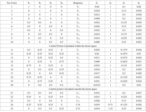
Table 6. The Determination of First 10 Mixes [Z n_]-1 _{Matrix Inverse Values Based On table 5}

Z1 Z2 Z3 Z4 Z1Z2 Z1Z3 Z1Z4 Z2Z3 Z2Z4 Z3Z4

95.90 100.80 283.60 79.90 -196.20 -39.30 87.70 -136.70 -18.40 -257.30

1.20 0.30 -5.80 -0.60 -2.30 -2.30 0.10 8.10 -1.50 2.90

11.80 0.90 -46.10 -0.90 -24.90 -12.30 -2.60 66.30 -3.80 11.70

-141.40 96.10 266.50 -40.70 172.90 339.70 -62.10 -786.00 103.90 51.30

-1.30 -1.30 -1.60 -0.70 2.60 1.40 -1.10 -0.70 0.80 2.00

-0.20 -0.30 -4.80 -0.90 0.60 -1.50 -0.20 5.10 -1.10 3.30

5.80 1.70 -33.20 -4.60 -7.80 -21.00 3.00 48.50 -11.80 19.50

-0.20 0.00 0.90 0.00 0.40 0.30 0.00 -1.20 0.10 -0.30

1.30 -1.00 -1.50 0.60 -1.40 -3.10 0.60 6.60 -0.80 -1.30

2.00 -0.90 -6.30 -0.30 -2.90 -4.20 0.30 11.90 -1.20 1.60

The UCS responses concedes for each blend proportion henceforth to create expectation as shown for 10 blends which satisfy the condition in equation (4) The UCS responses are:

�𝑌𝑌(𝑛𝑛)_�=

⎣ ⎢ ⎢ ⎢ ⎢ ⎢ ⎢ ⎢ ⎢ ⎡1394.3₁₃₇₃

1361.1 1338.6 1371.8 1381.2 1363.7 1331.8 1328.7 1321.7⎦⎥

⎥ ⎥ ⎥ ⎥ ⎥ ⎥ ⎥ ⎤

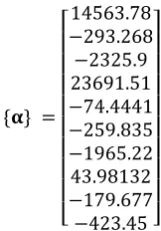
[image:8.595.57.541.89.404.2] [image:8.595.59.544.425.587.2]

{𝛂𝛂} =

⎣ ⎢ ⎢ ⎢ ⎢ ⎢ ⎢ ⎢ ⎢

⎡₋14563.78_293.268 −2325.9 23691.51

−74.4441

−259.835

−1965.22 43.98132

−179.677

−423.45⎦⎥

⎥ ⎥ ⎥ ⎥ ⎥ ⎥ ⎥ ⎤

By substituting the values of α into equation 4 then the prediction model at the response of UCS is:

𝑌𝑌= 14563.78𝑧𝑧1−293.268𝑧𝑧2−2325.9𝑧𝑧3+ 23691.51𝑧𝑧4−

74.4441𝑧𝑧1𝑧𝑧2−259.835𝑧𝑧1𝑧𝑧3−1965.22𝑧𝑧1𝑧𝑧4+

43.98132𝑧𝑧2𝑧𝑧3−179.677𝑧𝑧2𝑧𝑧4−423.45𝑧𝑧3 (8)

4.7. Statistical Verification for Model Adequacy

To verify whether the mathematical model in equation 8 is adequate to be used to predict UCS, it is necessary to run statistical test and compare the results from the prediction model with experimental results. F-test is common method to verify the adequacy of the model. The following hypotheses are prescribed as follows:

H0 denotes the statistical Null Hypothesis.

H1 represents the alternative Hypothesis.

The hypothetical condition is that H0 there are no

significance differences between the observed data and the data calculated from mathematical model however H1

signifies that there is statistical difference between the experimental data and data calculated from mathematical model.

To pursue that, the samples are yet called Y(observed) from

experimental data and Y(predict) from mathematical model.

Variance is calculated by the following equation:

𝑣𝑣2_{= �} 1

𝑛𝑛−1�[∑(𝑌𝑌 − 𝑦𝑦)2] (9) 𝑦𝑦=∑ 𝑌𝑌_𝑛𝑛 (10) In which, n is the number of responses of the analysis. According to table 7 the variances are calculated as follows:

𝑣𝑣𝑝𝑝𝑝𝑝𝑝𝑝𝑝𝑝2 =367₁₄.925= 26.28

𝑣𝑣𝑜𝑜𝑜𝑜2 =363₁₄.67=25.98

The fisher test is given by:

𝐹𝐹=𝑣𝑣12

𝑣𝑣22 (11)

𝐹𝐹=26₂₅._.28₉₈= 1.01

Referring to the F-distribution tables F0.95(14,14) = 2.48

which is higher than 1.01 therefore the null hypothesis (H0)

is not rejected and the mathematical model is considered adequate and verified to predict UCS for mix contains POFA-OPC additives.

Table 7. F-Test Analysis Prediction Model

Sample No Y observed

(kPa) Y(kPa) predicted Y(ob)(kPa) -y(ob) Y(pred)(kPa) -y(pred) (Y(obs) -y (obs) )

2

(kPa) (Y(pred) -y(pre) )

2

(kPa)

C1 1316.40 1374.85 -11.67 12.32 136.19 151.81

C2 1322.60 1359.14 -5.47 -3.39 29.92 11.48

C3 1312.90 1329.17 -15.17 -33.36 230.13 1112.82

C4 1343.20 1372.12 15.13 9.59 228.92 92.05

C5 1335.70 1358.75 7.63 -3.78 58.22 14.27

C6 1354.70 1336.87 26.63 -25.66 709.16 658.64

C7 1361.20 1355.66 33.13 -6.87 1097.60 47.18

C8 1326.10 1399.07 -1.97 36.54 3.88 1334.95

C9 1312.60 1414.52 -15.47 51.99 239.32 2702.68

C10 1361.20 1339.83 33.13 -22.70 1097.60 515.20

C11 1302.30 1337.60 -25.77 -24.93 664.09 621.69

C12 1309.40 1353.27 -18.67 -9.26 348.57 85.66

C13 1318.70 1409.97 -9.37 47.44 87.80 2250.79

C14 1313.90 1357.22 -14.17 -5.31 200.79 28.19

C15 1330.20 1339.83 2.13 -22.70 4.54 515.20

Total 19921.10 20437.88 5136.71 10142.60

[image:9.595.133.214.78.194.2]

5. Conclusions

This study has developed mathematical model to predict UCS for mixes containing organic soil stabilized by POFA POFA-OPC additives. The model was verified statistically and has shown adequate to be used for further investigation. This model was aimed to save time and cost in optimizing the contents of additives and can avoid arbitrary selection of percentages. Yet, it is suggested that this technique can be used in many materials optimization applications.

Acknowledgements

Authors acknowledge the assistance and financial support provided the ministry of higher education Yemen. It also goes to the University Tun Hussein Onn Malaysia for the laboratory facilities and assistance.

REFERENCES

[1] Tasnimi, A. A. (2004). Mathematical model for complete stress–strain curve prediction of normal, light-weight and high-strength concretes. Magazine of concrete research, 56(1), 23-34.

[2] Scheffe, H. (1958). Experiments with Mixtures. Journal of the Royal Statistical Society, Series. B., 20, 344 – 360. [3] Mbadike & Osadebe (2013). “Application of Scheffe’s

model in optimization of compressive strength of lateritic concrete”. Journal of Civil Engineering and Construction Technology, 4(9).

[4] D.O. Onwukaa, Okerea, Arimanwaa and S.U. Onwukab (2011) “Prediction of concrete mix ratios using modified regression theory “Comp. Meth. Civil Eng., Vol. 2 No. 1, pp. 95-107.

[5] C.E. Okere, D.O. Onwuka, S.U. Onwuka, J.I. Arimanwa, (2013) "Optimisation of concrete mix cost using Scheffe’s simplex lattice theory" Journal of Innovative Research in Engineering and Sciences 4(1), February, 2013. ISSN: 2141-8225 (Print); ISSN: 2251-0524 (Online)

[6] Gamil, Y. M. R., & Bakar, I. H. (2016, July). The Development of Mathematical Prediction Model to Predict Resilient Modulus for Natural Soil Stabilized by Pofa-Opc Additive for the Use in Unpaved Road Design. In IOP Conference Series: Materials Science and Engineering (Vol. 136, No. 1, p. 012007). IOP Publishing.

[7] Ming, K. K., & Chandramohan, D. (2002). "Malaysian palm oil industry at crossroads and its future direction". Oil Palm Industry Economic Journal, 2(2), 10-15.

[8] Shuit, S. H., Tan, K. T., Lee, K. T., & Kamaruddin, A. H. (2009). Oil palm biomass as a sustainable energy source: A Malaysian case study. Energy, 34(9), 1225-1235.

[9] European Union Report. (2012). “The Malaysian Palm Oil

Sector –Overview.” report (June): 1–53.

[10]Yaser Gamil, Ismail & Kemas (2015)” Optimization of the use of POFA to improve palm oil plantation road” Master dissertation, University Tun Hussein Onn Malaysia.

[11]Tangchirapat, W., Saeting, T., Jaturapitakkul, C., Kiattikomol, K., & Siripanichgorn, A. (2007). "Use of waste ash from palm oil industry in concrete". Waste Management, 27 (1), 81-88. Available at: http://www.ncbi.nlm.nih.gov/pubmed/16497498 [Accessed March 20, 2013].

[12]Ma, A. N., & Ong, A. S. (1985). Pollution control in palm oil mills in Malaysia. Journal of the American Oil Chemists’ Society, 62(2), 261-266.

[13]Sata, V., Jaturapitakkul, C. & Kiattikomol, K., (2004). "Utilization of Palm Oil Fuel Ash in High-Strength Concrete"., (December), pp.623–628.

[14]Altwair, N.M., Johari, Megat A Megat & Hashim, Syed F Saiyid, (2011). "Influence of Calcination Temperature on Characteristics and Pozzolanic Activity of School of Materials and Mineral Resources Engineering”, Engineering Campus., 5(11), pp.1010–1018.

[15]Tay, J., (1990). "Ash from Oil Palm Waste as a Concrete Material". Journal of Materials in Civil Engineering, 2(2), pp.94–105. Available at:

http://ascelibrary.org/doi/abs/10.1061/%28ASCE%290899-1561%281990%292%3A2%2894%29.

[16]Hussin, Mohd Warid, Muthusamy, K. & Zakaria, F., (2010). "Effect of Mixing Constituent toward Engineering Properties of POFA Cement-Based Aerated Concrete". , (April), pp.287–295.

[17]K.Abdullah, M.W.H., (2006). "POFA: A Potential Partial Cement Replacement Material In Aerated Concrete.”, (September), pp.5–6.

[18]Tay, J. H., & Show, K. Y. (1995). "Use of ash derived from oil-palm waste incineration as a cement replacement material, Resources, conservation and recycling", 13(1), 27-36.

[19]Awal, A. A., & Hussin, M. W. (1997). The effectiveness of palm oil fuel ash in preventing expansion due to alkali-silica reaction. Cement and Concrete Composites, 19(4), 367-372.

[20]Radin Sumadi, S., Chan, P. C., & Jasmin, L. S. (2006). "Blended cement for waterproofing applications".

[21]Eldagal, A., & Elmukhtar, O. (2008). Study on the behaviour of high strength palm oil fuel ash (POFA) concrete (Doctoral dissertation, University Technology Malaysia, Faculty of Civil Engineering).

[22]Tangchirapat, W., Jaturapitakkul, C., & Chindaprasirt, P. (2009). Use of palm oil fuel ash as a supplementary cementitious material for producing high-strength concrete. Construction and Building Materials, 23(7), 2641-2646. [23]Phani Kumar, B. R., & Sharma, R. S. (2004). "Effect of fly

ash on engineering properties of expansive soils".Journal of Geotechnical and Geoenvironmental Engineering, 130(7), 764-767.

H. (2015). Stabilization of clayey soil using ultrafine palm oil fuel ash (POFA) and cement. Transportation Geotechnics, 3, 24-35.

[25]Oades, J. M. (1984). Soil organic matter and structural stability: mechanisms and implications for management. In Biological Processes and Soil Fertility (pp. 319-337). Springer Netherlands.

[26]Farnham, R. S., & Finney, H. R. (1965). Classification and properties of organic soils. Advances in Agronomy, 17, 115-162.

[27]Sollins, P., Homann, P., & Caldwell, B. A. (1996). Stabilization and destabilization of soil organic matter: mechanisms and controls. Geoderma, 74(1-2), 65-105. [28]Tastan, E. O., Edil, T. B., Benson, C. H., & Aydilek, A. H.

(2011). Stabilization of organic soils with fly ash. Journal

of geotechnical and Geoenvironmental Engineering, 137(9), 819-833.

[29]ASTM D2166-06. 2003, “Standard Test Method of Unconfined Compressive Strength of Cohesive Soil”. Astm Int'L.

[30]ASTM C136-96a, Standard Test Method for Sieve Analysis of Fine and Coarse Aggregates, ASTM International, West Conshohocken, PA, 2001, www.astm.org

[31]ASTM C618. Standard specification for coal fly ash and raw or calcined natural pozzolan for use as a mineral admixture in concrete. Annual book of ASTM standards, vol. 04.02; 2001. p. 310–3.