Approximate Analysis of Transient Heat Conduction in
the Stator of an Induction Motor during
Auto-transformer Starting
D. Sarkar1,*, N.K. Bhattacharya2, A.K. Naskar3
1
Department of Electrical Engineering, Indian Institute of Engineering Science and Technology (IIEST), India
2
Department of Physics, Faculty Council of Science, Jadavpur University (JU), India
3
Department of Electrical Engineering, Techno India-Batanagar (TI-B), India
Copyright©2017 by authors, all rights reserved. Authors agree that this article remains permanently open access under the terms of the Creative Commons Attribution License 4.0 International License
Abstract
For the development of electric machines, particularly induction machines, temperature limit is a key factor affecting the efficiency of the overall design during transient state. Since conventional loading of induction motors is often expensive, the estimation of temperature rise by tools of mathematical modeling becomes increasingly important and as a result of which computational methods are widely used for estimation of temperature rise in electrical machines. This paper describes the problem of two dimensional transient state heat flow in the stator of induction motor during auto-transformer starting. The stator being static is prone to high temperature and the study of thermal behavior in the stator is useful to identify the causes of failure in induction machines. The temperature distribution is obtained using finite element formulation and employing arch shaped elements in the r-θ plane of the cylindrical co-ordinate system. This model is applied to one 3-phase squirrel cage induction motor of 7.5 kW rating.Keywords
Induction Motor, FEM, Temperature Rise, Insulation, Thermal Analysis, Transient, Design Performance1. Introduction
Considering the extended use of squirrel cage induction machine in industrial or domestic applications both as motor and generator, the improvement of the energy efficiency of this electromechanical energy converter represents a continuous challenge for the design engineers. Any achievements in this area mean important energy savings for the world economy. Thus, to design a reliable and economical motor, accurate prediction of temperature distribution within the motor and effective use of the coolant
for carrying away the heat generated in the iron and copper are important to designers [1]. Traditionally, thermal studies of electrical machines have been carried out by analytical techniques, or by thermal network method [2, 3]. These techniques are useful when approximations to thermal circuit parameters and geometry are accepted. Numerical techniques based on either finite difference method [4, 5] or finite element method [6-8, 9-13] are more suitable for analysis of complex system. Rajagopal et al. [14, 15] carried out two-dimensional steady state and transient thermal analysis of TEFC machines using FEM. Compared to the finite difference method, finite element method can easily handle complicated boundary configurations and discontinuities in material properties. The finite element method is first introduced for the steady state thermal analysis of the stator cores of large turbine-generators by Armor and Chari [16]. However, their works are restricted to core packages far from the ends and they do not consider the influence of the stator coil heat. Armor [17] employed arch-shaped finite elements to solve the transient heat flow in the rotor of large turbine-generators. Sarkar [18] also described a method based on arch-shaped finite elements with explicitly derived solution matrices for determining the thermal field of induction motors.
Use of finite elements has seldom been attempted due to the complexity and high cost of computation and detailed 2-dimensional transient thermal analysis is not known to be reported for auto-transformer starting of induction motors.
at mid-slot, mid-tooth divided into 24 arch shaped elements and thus provides a new approach of multi-time interval solution to a transient stator heating problem and this defines the scope of this technique. The requirements of computer storage for a large number of elements have been reduced by the use of half band- width of the symmetric matrix.
The method is directly applicable to the study of temperature rise during auto-transformer starting that may arise following some intentional starting actions. The procedure is particularly suited to the study of transient heating of the stator coils due to I2R losses in the coil slots during auto-transformer starting.
2. Finite Element Formulation
The general form of the heat conduction equation can be described by the following relations
(1) Where, T is the potential function (temperature), V is the medium permeability (thermal conductivity), q is the flux (heat flux), Q is the forcing function (heat source), Pm and Cm are material density and specific heat respectively.
In cylindrical polar co-ordinates, equation (2) can be expanded as
(2) Where, Vr, Vθ are thermal conductivities in the radial and
circumferential directions respectively.
2.1. Finite Element Analysis (Galerkin’s Method)
The Galerkin’s criterion is used for obtaining approximate solutions to linear and non-linear partial differential equations. When only the governing differential equations and their boundary conditions are available, Galerkin’s method is convenient in a way that this approach surpasses the variational method in generality and further broadens the range of applicability of the finite element method. Though the element equations derived for those problems were explicitly evaluated only for the simplest type in each case, the equations are general and be applied for many element shapes and displacement models. The popularity of the method stems mainly from the case with which irregular geometries and implicit natural boundary conditions can be handled. Another important advantage is that the method allows development of general computer program that can solve variety of thermal problems simply by accepting different input data. The computer program illustrates how a real problem is actually solved by finite element method. It is envisaged that such programs would be useful for future studies of more complicated problems.
The solution of equation (3) can be obtained by assuming
the general functional behavior of the dependent field variable in some way so as to approximately satisfy the given differential equation and boundary conditions. Substitution of this approximation into the original differential equation and boundary condition then results in errors called a residual. This residual is required to vanish in some average sense over the entire solution domain.
The approximate behavior of the potential function within each element is prescribed in terms of their nodal values and some weighting functions N1, N2 ... such that
i=1, 2… m (3) The weighting functions are strict functions of the geometry and are termed interpolation functions. These interpolation functions determine the order of the approximating polynomials for the heat conduction problem.
The method of weighted residuals determine the ’m’ unknowns Ti in such a way that the error over the entire solution domain is small. This is accomplished by forming a weighted average of the error and specifying that this weighted average vanishes over the solution domain.
The required equations governing the behavior of an element is given by the expression
(4) Where, T0 is the temperature at the previous point in time and ∆t is the time interval
Equation (4) expresses the desired averaging to the error or residual within the element boundaries, but it does not admit the influence of the boundary. Since we have made no attempt to choose the Ni so as to satisfy the boundary conditions, we must use integration by parts to introduce the influence of the natural boundary conditions.
2.2. Arch Element Shape Functions
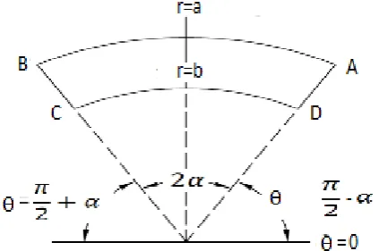
Consider the arch-shaped element of Figure 1 formed by circle arcs radii a, b, radii inclined at an angle 2α.
Figure 1. 2-D Arched shaped element suitable for discretization of induction motor stator
2
m m
T
V T P C Q
t
δ
δ
∇ = − 2 2 2 1 0r m m
V
T T T
V r Q P C
r r r r t
θ
δ δ δ δ
δ δ δθ δ
+ + − =
i i
T = ΣN T
( ) ( )
( )
( ) (e) 0 2 2 2 0 2 e
e e e
i r m m
D
V T T
T T
N V Q P C rdrd
r r r t
θ
δ δ δ δ θ
δ δ δθ δθ
+ + − − =
∆
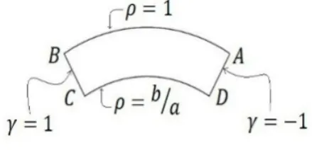
[image:2.595.329.541.584.724.2]The shape functions can now be defined in terms of a set of non-dimensional coordinates with the help of cylindrical polar coordinates r, θ using the formula given below
ρ =ra , γ =θ − π 2α �
[image:3.595.67.287.190.296.2]The arch element with non-dimensional co-ordinates is shown in Figure 2.
Figure 2. The non-dimensional arch shaped element
The temperature at any point within the element be given in terms of its nodal temperatures by
T = TANA+ TBNB+ TCNC+ TDND (5) Where the N’s are shape functions chosen as follows:
; ) 1 ( 2 ) 1 )( ( a b a b A N − − − − = γ ρ ; ) 1 ( 2 ) 1 )( 1 ( a b C N − − + −
= ρ γ
; ) 1 ( 2 ) 1 )( ( a b a b B N − + − = γ ρ ) 1 ( 2 ) 1 )( 1 ( a b D N − − −
= ρ γ
(6)
It is seen that the shape functions satisfy the following conditions:
(i) That at any given vertex ’A’, the corresponding shape function NA has a value of unity and other shape functions NB,NC have a zero value at this vertex. Thus, at node j, Nj = l but Ni =0, i≠j.
(ii) The value of the potential varies linearly between any two adjacent nodes on the element edges.
(iii) The value of the potential function in each element is determined by the order of the finite element. The order of the element is the order of polynomial of the spatial co-ordinates which describes the potential within the element. The potential varies as a quadratic function of the spatial co-ordinates on the faces and within the element.
2.3. Boundary Conditions
The temperature distribution is assumed symmetrical across two planes, with the heat flux normal to the two surfaces being zero. From the other two boundary surfaces, heat is transferred by convection to the surrounding gas. It is converted to the air gap gas from the teeth, to the back of core gas from the yoke iron. The boundary conditions may be written in terms of
δ
T/δ
n, the temperature gradient normal to the surface.Mid-slot surface 0 = s n T δ δ
Mid- tooth surface
0 = t n T δ δ
Air gap surface
AG δn δT -V ) h (T-T r AG =
Back-of-core surface, BC r nBC
T V T
T
h( − ) = − δδ
Where, T=Surface temperature, TAG= Air gap gas
temperature and TBC = Back of core gas temperature
2.4. Approximate Numeric Form
(7)
Where nr is the r component of the unit normal to the boundary, and d∑ is a differential arc length along the boundary. Equation (6) takes the form
(8)
There are four such equations as (7) for the four vertices of the element. These equations, when evaluated, lead to the matrix equation
(9)
Where, [SR], [Sθ] are symmetric coefficient matrices (thermal stiffness matrices),[SH] is the heat convection matrix, [ST] is the heat capacity matrix, [T] is the column vector of unknown temperatures, [T0] is the column vector of unknown (previous point in time) temperatures, [R] is the forcing function (heat source vector), and [SC] is the column vector of heat convection.
3. Discretized Model for FEM
Application
The stator of an induction motor being static is prone to high temperature and the temperature distribution of the stator only is computed here .The hottest spot is generally in the copper coils. Thermal conductivity of copper and insulation in the slot are taken together for calculation. As the temperature is the maximum at the central plane, the temperature distribution in the plane can be determined approximately by taking this as a two-dimensional r-θ problem with the following assumptions:
(a) The temperature in the strip of unit thickness on the central axis is assumed to be fixed axially i.e. no axial flow of heat is assumed in the central plane. This assumption is permissible because in the central plane where the temperature distribution is the maximum, while the temperature gradient in the axial direction is zero.
(b) The convection is taken care of only at the cylindrical surfaces neglecting the convection at the end surfaces. Because of this assumption, the temperatures calculated in the central plane will be slightly higher than the actual.
In the case of transient stator heating caused by auto transformer starting, the transient analysis procedure is able to provide an estimate of the temperatures throughout the
volume of the stator at an interval of time required to bring the motor from rest to rated speed by providing reduced voltage when auto transformer is connected in the circuit and rated voltage when auto transformer is disconnected from the circuit during starting action,
Assuming that the machine is at rest with its stator winding at normal ambient temperature, respective voltage and current are injected to the stator winding of the machine. The temperatures within the volume of the stator are calculated at the nodal points for a period of the time required for starting action.
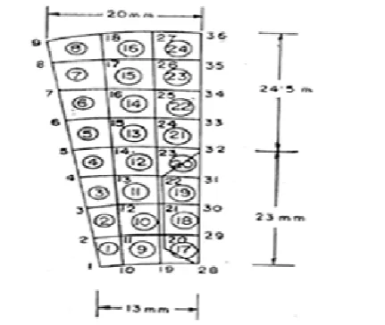
Figure 3. Slice of armature iron and winding bounded by planes at mid-slot and mid-tooth divided into arch-shaped finite elements.
In this analysis because of symmetry, the two-dimensional domain in cylindrical polar co-ordinates of core iron and winding, chosen for modeling the problem and the geometry is bounded by planes passing through the mid-tooth and the mid-slot, which are divided into finite elements as shown in
[ ] [ ] [ ] [ ] [ ] [ ][ ] [ ] [ ]
S
RS
θS
TS
HT
S
TT
0R
S
C
+
+
+
=
+
+
[image:4.595.324.540.469.651.2]Figure 3. Arch-shaped elements are used throughout the solution region.
4. Calculation of Heat Losses [19]
Heat losses in the stator tooth and core are determined on calculated magnetic flux densities (0.97wb/m2 and 1.293wb/m2 respectively) in these regions, tooth flux lines are predominantly radial and yoke flux lines predominantly circumferential. The gain orientation of the core punching varies in these two directions and therefore influences the heating for a given flux density. Copper losses in the winding are determined from the length as well as the area required for the conductors in the slot.
Iron loss of stator core per unit volume = 3.88708×10⁻⁵W/mm3.
Iron loss of stator teeth per unit volume=3.92352×10⁻⁵W/mm3.
4.1. Stator Copper Loss
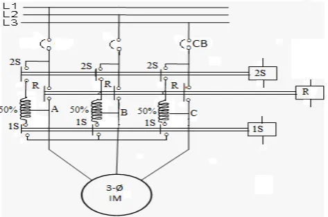
These types of starters use an auto-transformer between the motor and the supply lines to reduce starting current of the motor. The auto-transformer may be single three phase type or three single phase type, for our case we will consider a single three phase type auto-transformer as shown in figure 4. Taps are provided on the auto-transformer to select 50%, 65%, and 80% of the line voltage of starting.
For the purpose of the auto–transformer starting contactors, 1S, and 2S are closed, as a result the transformer is energized from the supply. Reduced voltage from taping A, B and C is available at the motor terminals. After the motor picks up sufficient speed contactor 1S is first de-energized. Auto-transformer’s neutral connection gets open circuited. The motor remains connected to supply through contacts of contactor 2S and the transformer acts as an impedance in the motor circuit. Next, the run contactor R is energized which bypasses the impedance and connects the motor directly to the supply.
[image:5.595.315.552.227.384.2]We are interested in auto-transformer starting of the induction motor, the equivalent circuit of which is shown in figure 5 to calculate the temperature distribution in the stator during the starting period. For the purpose of starting, we will take the starting voltage at 50% of full voltage to start with and calculations will be done on that voltage till the auto-transformer acts as impedance in the motor circuit. Finally, the temperature distribution within the stator due to reduced voltage auto-transformer starting are calculated by splitting the entire slip range (i.e. from s=1 to full load slip s=0.04) into small intervals.
[image:5.595.312.553.411.517.2]Figure 4. Power circuit for a line auto-transformer reduced voltage starter
Figure 5. Equivalent Circuit of Induction Motor
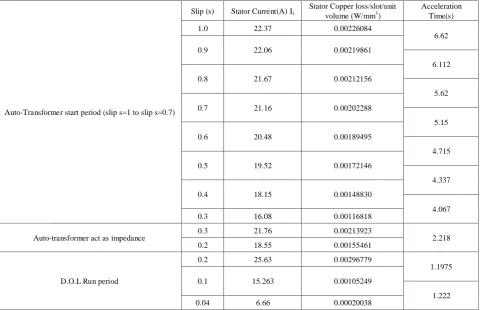
Table 1. The different values of stator current, stator copper loss/slot/unit volume and time required for starting action at different slips in auto-transformer starting
Auto-Transformer start period (slip s=1 to slip s=0.7)
Slip (s) Stator Current(A) I1
Stator Copper loss/slot/unit volume (W/mm3)
Acceleration Time(s) 1.0 22.37 0.00226084
6.62 0.9 22.06 0.00219861
6.112 0.8 21.67 0.00212156
5.62 0.7 21.16 0.00202288
5.15 0.6 20.48 0.00189495
4.715 0.5 19.52 0.00172146
4.337 0.4 18.15 0.00148830
4.067 0.3 16.08 0.00116818
Auto-transformer act as impedance 0.3 21.76 0.00213923 2.218 0.2 18.55 0.00155461
D.O.L Run period
0.2 25.63 0.00296779
1.1975 0.1 15.263 0.00105249
1.222 0.04 6.66 0.00020038
4.2. Convective Heat Transfer Co-efficient [1, 2]
Two separate values of convective heat transfer co-efficient have been taken for the cylindrical curved surface over the stator frame and the cylindrical air gap surface. The natural convection heat transfer co-efficient on cylindrical curved surface over the stator frame is taken as h=5.25W/m2°C.The heat transfer co-efficient on forced convection for turbulent flow in cylindrical air gap surface is taken as h=60.16W/m2°C.
4.3. Thermal Constants [1]
For the transient problem in two dimensions, the following properties are taken for each different element material.
Table 2. Typical Set of Material Properties for Induction Motor stator
Magnetic Steel Wedge Copper &Insulation
Vr 33.070 2.007
Vθ 0.8260 1.062
Pm 7.86120 8.9684
Cm 523.589 385.361
5. Results and Discussions
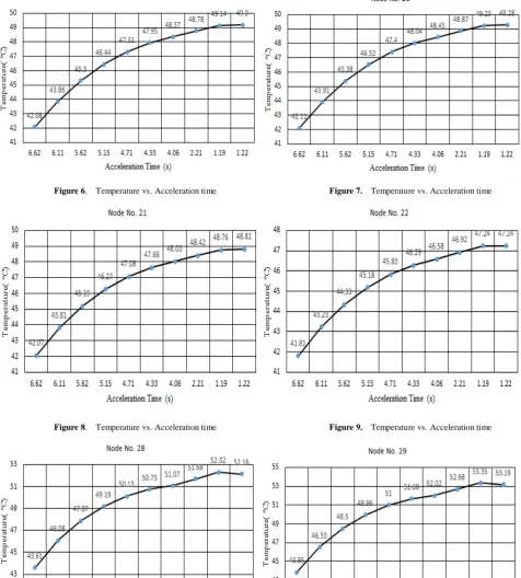
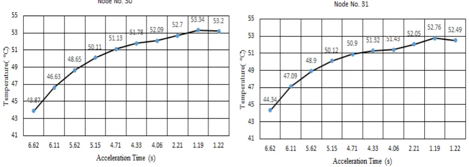
Since the hottest spots are found to be in the stator copper as envisaged from the calculated temperatures for the two-dimensional structure during the auto-transformer starting period, the temperature variation with time in each node of copper is taken as an index to understand the temperature profile during the transient. It is to be noted that the temperature is found to be the maximum at the nodes pertaining to copper in the axis of symmetry. The temperature rise is steady at different stator currents under the auto-transformer starting region at different slips from s = 1 to s = 0.2. It is also to be noted that under DOL run the motor has reached a steady speed under full load condition and as such there is a slight decrease of hot spot temperatures persisting across the axis of symmetry after the motor is directly connected across the supply.
[image:6.595.59.298.652.725.2]Figure 6. Temperature vs. Acceleration time Figure 7. Temperature vs. Acceleration time
Figure 8. Temperature vs. Acceleration time Figure 9. Temperature vs. Acceleration time
[image:7.595.72.540.491.664.2]Figure 12. Temperature vs. Acceleration time Figure 13. Temperature vs. Acceleration time
6. Conclusions
The two-dimensional transient finite element procedure for the thermal analysis of large induction-motor stator provides the opportunity for the in-depth studies of stator heating problems. By virtue of the new, explicitly derived arch shaped element, together with an efficient bandwidth and Gauss routine, extremely large problems can be efficiently solved.
A new two-dimensional finite element procedure in cylindrical polar co-ordinates, with explicitly derived solution matrices, has been applied to the solution of the transient heat conduction equation during auto-transformer starting. Though the results are approximate, the method is fast, inexpensive and leads itself to immediate visual pictures of the temperature pattern in a two-dimensional slice of core and winding in the stator of an induction motor.
REFERENCES
[1] Griffith, J.W., R.M. Mc. Coy and D.K.Sharma (1986). Induction motor squirrel cage rotor winding thermal analysis.
IEEE Trans. on EC, EC-1, 22-25.
[2] Okoro, O.I. (2005).Steady and transient states Thermal Analysis of a 7.5 KW Squirrel cage Induction Machine at Rated Load Operation. IEEE Trans. Engg Convers, vol.20, 730-736.
[3] Rosenberry Jr., G.M. (1955).The transient stalled temperature rise of cast aluminum squirrel-cage rotors for induction motors.
AIEE Trans., PAS-74, 819-824.
[4] Reichert, K. (1969).The calculation of the temperature distribution in electrical machines with the aid of the finite difference method. Elektro Tech Z-A, Bd 90, H6.
[5] Tindall, C.E. and S. Brankin. (1988). Loss-at-source thermal modeling in salient pole alternators using 3- dimensional finite difference techniques. IEEE Trans. Magnetics, 24, 279-281.
[6] Naskar, A.K and Sarkar, D.(2015) Computational Analysis Of Three Dimensional Steady State Heat Conduction In The Rotor Of An Induction Motor By Finite Element Method.
Latin American Applied Research 45 (4), 245-253.
[7] Sarkar, D and Naskar, A.K. (2014) .Computation of thermal condition in an induction motor during plugging. International Journal of Power and Energy Conversion 5 (2), 172-196.
[8] Demoulias, C., D.P. Labridis, P. Dokopoulos and K. Gouramanis (2008). Influence of metallic trays on the ac resistance and ampacity oflow voltage cables under non sinusoidal currents. Electric Power Systems Research, vol. 78, 883-896.
[9] Holman, J.P. (1997). Heat Transfer, McGraw-Hil, New York
[10] Huebner, K.H., E.A. Thorton and T.G. Byrom. (1995). The Finite Element Method for Engineers, John Wiley & Sons, 3rd ed.
[11] Hwang, C.C. and C.T. Pan. (1988). Comparison of finite element methods for the diffusion problem. Int. J. Systems Sci., 119, 1165–1179.
[12] Lin, R. and A. Arkkio. (2008).3-D finite element analysis of magnetic forces on stator end-windings of an induction machine. IEEE Transactions on Magnetics, 44, 4045–4048.
[13] Sarkar, D and Naskar, A.K. (2014). Computation of Thermal Condition in an Induction Motor during Direct-On-line Starting. Journal of Electrical Engineering 12 (4), 1-12.
[14] Rjagopal, M.S., D.B. Kulkarni, K.N. Seetharamu and P.A. Ashwathnarayana. (1994). Axisymmetric steady state thermal analysis of totally enclosed fan cooled induction motors using FEM. 2nd Nat. Conf. on CAD/CAM.
[15] Rajagopal, M.S., K.N. Seetharamu and P.A. Ashwathnarayana. (1998). Transient thermal analysis of induction Motors. IEEE Trans. Energy conversion, vol. 13, pp. 62- 69.
[17]Armor, A.F. (1980). Transient, three-dimensional, finite element analysis of heat flow in turbine-generator rotors. IEEE Trans., PAS-99, 934–946.
[18]Sarkar, D. (1997).Approximate analysis of temperature rise in
an induction motor during dynamic Braking. Electric Machine and Power Systems, vol. 25, 57-71.