Quantitative Reasoning Process in Mathematics
Problem Solving: A Case on Covariation Problems
Reviewed from APOS Theory
Syarifuddin1,2,*, Toto Nusantara3, Abd. Qohar3, Makbul Muksar3
1State University of Malang, Indonesia
2Department of Mathematics Education, STKIP Bima, Indonesia
3Faculty of Mathematics and Natural Science, State University of Malang, Indonesia
Received July 25, 2019; Revised September 9, 2019; Accepted September 26, 2019
Copyright©2019 by authors, all rights reserved. Authors agree that this article remains permanently open access under the terms of the Creative Commons Attribution License 4.0 International License
Abstract The focus of this study was to describe the
students' quantitative reasoning process in solving covariate problems using APOS theory. This research was a case study conducted on 9th grade students of junior high schools in five different schools in Bima Regency, Indonesia. The data collection in this study was initially done by providing Covariation Problem Task (CPT) for students in a 60-minute task. Afterwards, it was followed up by holding task-based interviews with students who performed different processes. These interviews were intended to confirm the existing mental process. The data obtained were analyzed by combining retrospective and continuous analysis, namely by analyzing work results and student interviews simultaneously, then thinking structures were described based on APOS theory. The results of this study showed two different students’ quantitative reasoning processes for covariation problems. First, the inductive quantitative reasoning process (IQRP) was conducted by linking the quantity involved in covariation problems and substituting it into the formula directly, without making any modeling. Second, the deductive quantitative reasoning process (DQRP) was conducted by connecting quantity through the process of mathematical modeling by producing formula equations. This study indicated that the students comprehended the situation caused by covariate quantity relationships and the process (reasoning) of how quantity values change together.Keywords Quantitative Reasoning, Mathematics
Problem Solving, Covariation Problems, APOS Theory1. Introduction
One of the objects of reasoning in mathematics concerns
the understanding of quantitative relationships [1]. The reasoning on quantitative relations deals with how students perceive quantity and connect quantities. An important aspect of mathematical ability is to look at problem situations as quantity networks and internal quantities, and then form a series of quantitative operations in determining a solution [2]. Further, it is explained that a quantitative operation refers to a mental operation that combines two or more conditions to produce a new quantity. According to Weber et al. [3], quantitative reasoning is a way to describe a student's mental actions in understanding mathematical situations, constructing quantities in certain situations, and then connecting, manipulating, and using quantity to create a coherent problem situation.
Quantitative reasoning in general and for assessment purposes is focused on problem solving. According to Dwyer et al [4], quantitative reasoning requires the use of mathematical content for the purpose of assessment and problem solving more generally. Furthermore, it is explained that there are six capabilities that mark quantitative reasoning in the problem solving process; they are: 1) reading and understanding the information provided in various forms, such as in the form of graphs, tables, geometric images, mathematical formulas or texts; 2) making boundaries from mathematical or statistical methods; 3) problem solving using arithmetic, algebra,
geometry, or statistical methods; 4)
interpretingquantitative information and drawing conclusions; 5) communicating quantitative information verbally, numerically, algebraically or graphically; and 6) estimating and checking the feasibility of answers.
operations and objects [5]. Similarly, it happens in interpreting and using quantity in understanding covariation problems. Several studies on covariate problems reveal some of the difficulties students encounter in understanding problems and drawing graphics. Carlson, Madison, & West [6] in their research on the readiness of students to learn calculus found that students were weak in their basic abilities and reasoning abilities. Only a few students with higher grades had readiness and were successful in calculus. Stalvey & Vidakovic [7] in their research on the relation of quantity by drawing cartesius graphs explained that not many students could describe the two-quantity relationship in interpreting dynamic events. Moreover, Yemen, Ulusoy, & Işıksa [8] discovered that
high-achieving students had difficulty in modeling dynamic functional situations including covariate quantities.
To support the readiness of students to face difficulties in college calculus, several studies have also been conducted on the problem of covariation to student studying in high school grade. In Johnson [9] research reveals that students can do reasoning numerically and non-numerically about variations in covariate quantities. Then in Johnson [10] study of student reasoning in interpreting graphs as they can make comparisons on the number of changes in quantity.
From some of the studies above, it shows the difficulties faced by students in producing and interpreting graphs of covariate quantities. Not many students are able to produce solutions or graphics properly if they only rely on non-numerical reasoning. While in numerical reasoning [9], students are not really involved in producing their own numbers used in building their reasoning. In this study the problem of covariation was seen as the quantities identified by students and then connected in the form of quantitative reasoning. In developing students' reasoning, it involves problem solving to determine conclusions from covariate quantities.
The mental construction of students' quantitative reasoning on these covariation problems was investigated using the APOS theory. As explained by Dubinsky [11] that the APOS theory is a constructivist framework based on reflective abstraction that emphasizes the construction of mental structures. In the mental structure of this theory, it consists of mental constructions (Action, Processes, Objects and Schemes) and mental mechanisms (interiorization, encapsulation, de-encapsulation, coordination, and reversa) [12]. This is applied in several studies, for example about concepts understanding and derivative graphs [13-15], principles of mathematical induction [16], as well as graph functions (calculus knowledge) [17]. Similarly, in this study, APOS was used to investigate mental structures in student reasoning on the problem of covariation and to graph the relationship between the quantities involved in it.
2. Materials and Methods
The type of research used is qualitative research with a descriptive explorative approach. Miles, Huberman, & Saldana [18] explained that qualitative research is done by dealing directly with participants (humans) in naturalistic settings to investigate extraordinary phenomena from individuals or groups. This study reveals the thinking process of students in developing quantitative reasoning in solving covariation problems. The process of developing quantitative reasoning is seen from the way students complete Covariation Problem Task (CPT).
2.1. Participants
The subjects involved in this study were 9th grade junior high school students from five different schools in Bima Regency, Indonesia. At each school, one class was taken and selected according to the recommendations of the mathematics subject teachers. The distribution of these subjects can be seen in Table 1.
Table 1. Distribution of subjects from five schools
No. School The number of students
1. Junior High School 1 25
2. Junior High School 2 23
3. Junior High School 3 28
4. Junior High School 4 26
5. Junior High School 5 30
Total 132
From each school, Subjects were then selected who could provide answers that indicated a different quantitative reasoning process to be explained in the results of the study. Subjects were selected based on several criteria, namely they were willing to be involved as the subjects and they had good verbal ability. The intention was that they can be the respondents in task-based interviews well.
2.2. Instrument
Figure1. The Covariation Problem Task (CPT)
2.3. Data Collection
CPT was used as a tool to obtain data on students' quantitative reasoning processes on covariation problems. The procedure of the study was carried out with the following stages: before the subject worked on the CPT, they were first explained the general purpose of the study that they will be used as the research subject, without explaining that they would be re-elected for the next stage based on their answers. The subject worked and completed the CPT independently for sixty minutes. The subjects’ answer sheets were corrected by referring to the indicators of the quantitative reasoning process that have been compiled as in table 2. The correction results are then categorized based on the process which shows different quantitative reasoning processes.
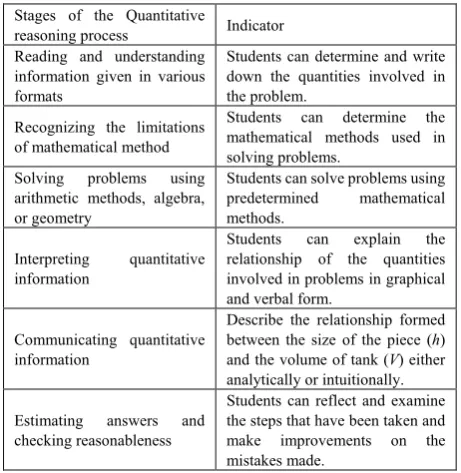
Table 2. Indicators of quantitative reasoning processes in solving covariation problem
Stages of the Quantitative
reasoning process Indicator
Reading and understanding information given in various formats
Students can determine and write down the quantities involved in the problem.
Recognizing the limitations of mathematical method
Students can determine the mathematical methods used in solving problems.
Solving problems using arithmetic methods, algebra, or geometry
Students can solve problems using predetermined mathematical methods.
Interpreting quantitative information
Students can explain the relationship of the quantities involved in problems in graphical and verbal form.
Communicating quantitative information
Describe the relationship formed between the size of the piece (h) and the volume of tank (V) either analytically or intuitionally.
Estimating answers and checking reasonableness
Students can reflect and examine the steps that have been taken and make improvements on the mistakes made.
To find out more about the quantitative reasoning
process, task based interviews were held. Interviews are conducted to confirm the mental processes carried out by the subjects. The interview process was carried out by means of the researchers dealing directly with the selected subject by confirming the steps to complete the CPT while showing the results of the subject's work. The data from interviews were collected by recording conversations using the help of a voice recorder and video recorder.
2.4. Data Analysis
The data obtained from the data collection process were in the form of answer sheets and results of task-based interview records. Both types of data were analyzed by combining retrospective and continuous analysis, and then thinking structures are described based on APOS theory. Retrospective analysis is used to review the process that has been done by the subject on the answer sheet. The initial stage uses coding to identify data when the subject forms and interprets covariate quantity relationships. The second stage uses comparative analysis [20], to compare each work result about the relationship between the quantities involved and make a difference between the ways the subject shapes and interprets the relationship between the quantities involved in the problem of covariation.
Continuous analysis includes reflective notes which are arranged after each interview. Continuous analysis informs task-based interviews which were carried out later with different subjects and the next iteration of the same task-based interviews with different subjects.
3. Results
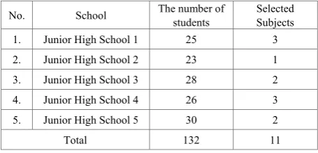
[image:3.595.132.468.85.173.2] [image:3.595.59.290.498.735.2]Table 3. Distribution of subjects from five schools and selected subject
No. School The number of students Selected Subjects
1. Junior High School 1 25 3
2. Junior High School 2 23 1
3. Junior High School 3 28 2
4. Junior High School 4 26 3
5. Junior High School 5 30 2
Total 132 11
In general, of the 132 students working on CPT, there were two different categories produced by students: the inductive quantitative reasoning process (IQRP) and the deductive quantitative reasoning process (DQRP). Of the 132 students, only 11 showed the correct reasoning process. Then out of 11 students, there were 7 students showing the quantitative reasoning process correctly and 4 people revealing the less precise results. The distribution of these subjects can be seen in Table 4.
Table 4. Subject distribution in the quantitative reasoning process
The Overall
Subject Inappropriate process
Quantitative Reasoning Process Inductive Deductive
11 4 3 4
Percentage
(100 %) 36,36 % 27,27 % 36,36 %
Out of three subjects (hereinafter referred to as: S1, S2, and S3) who showed an IQRP, it was only described the process of one subject namely S1. On the other hand, the other four subjects (hereinafter referred to as: S4, S5, S6, and S7) who showed DQRP, it was only explained the process of one subject namely S4. Each Subject was taken from the two processes because the subject revealed the same process from the subject representing IQRP and DQRP.
3.1. Inductive Quantitative Reasoning Process (IQRP) At the action stage, S1 understood physical transformation from square (metal sheet) to beam shape (tank of water) by identifying the quantities involved in the problem. S1 wrote the quantities involved, namely the length, width, height, and volume of water that is written in the form of a volume formula for a beam, as shown in Figure 2. Then S1 interpreted the quantitative information of the problem by recording changes in the value of the size of the sheet metal corner pieces and the changes that occur in the related quantity. For example, the size of the pieces of the four angles is 0.1 (which is the height of the beam), so that the beam length is the length of the sheet metal reduced by the size of the pieces from both angles (for example: l = 2 – 2(0.1) = 2 – 0.2 = 1.8). Likewise, the next cut size can be seen from the work of S1 in Figure 3. In addition, S1 believed that the quantity of length is equal to the width (l = w). This can be seen from the S1 statement on the following script:
Int.: try to pay attention to the value of the length and width you wrote, what can you conclude from that?
S1: the value of length and width is always the same for each piece because the basic shape is square.
Note: Volume formula V = l × w × h p = length (l); l = width (w); t = height (h)
Figure 2. S1 wrote the volume formula of the beam which contains the volume, length, width, and height quantity.
Text translations: There are four corner pieces from
square metal sheets → which show the value of h, which is 0.1 meters, 0.2 meters, 0.3 meters, 0.4 meters, which is the same amount of angle pieces. ↓
[image:4.595.60.288.92.202.2] [image:4.595.97.505.557.691.2]At the process stage, S1 internalizes the action by solving problems using mathematical methods. The method is to calculate the quantity value in the next change of pieces. The values of the quantities that have been obtained are then substituted directly by the volume. This can be seen in Figure 4.
Figure 4. S1 substituted the quantity value (l, w, and h) to the volume formula
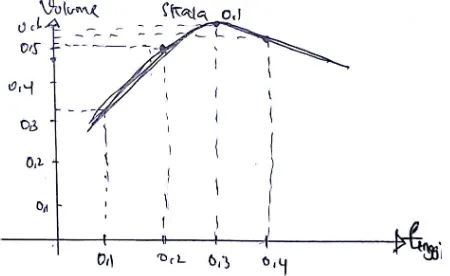
At the object stage, S1 encapsulates the process that has been done by coordinating the quantities that have been obtained into a graphic image, which shows the relationship of these quantities. The detail can be seen in Figure 5.
Figure 5. S1 coordinated the quantity between the size of the piece (h) and the volume of the tank (V)
In the scheme stage, S1 re-checked what had been done starting from the stages of action, process, and object. When he was asked about the image produced, the subject showed some doubt with the resulting graph. This was based on the results of interviews conducted with S1.
Int.: Are you sure of the image produced?
S1: Hmmm [while thinking and seeing the image it produces]
Int.: What is the volume of the tank if the cut size is 0 (zero) and the size of the pieces is 1 meter?
S1: ... [calculate the volume value], for the discount 0 the volume is equal to 0 pack and for the 1 meters volume the 0 is also pack [see Figure 6].
S1: Ooowwh ... it means the graph starts from zero point zero [0,0] and ends at one point zero [1,0].
[image:5.595.64.274.163.341.2]Besides, S1 completed the coordinate point (cut size) that had not been predetermined to perfect the previous image. The sizes of the pieces included 0.5 meters, 0.6 meters, 0.7 meters, 0.8 meters and 0.9 meters. Following are excerpts submitted by S1:
[image:6.595.64.289.179.353.2]S1: to complete the graph coordinates, I add the volume count at 0.5 meters, 0.6 meters, 0.7 meters, 0.8 meters and 0.9 meters [these coordinates can be seen on Figure 7].
Figure 7. S1 redrew the t and V coordination chart
[image:6.595.352.495.197.401.2]3.2. Deductive Quantitative Reasoning Process (DQRP) At the action stage, S4 understood the problem as carried out by S1 above, which was to understand the physical transformation from a square (metal sheet) to a beam (water tank) by identifying the quantities involved in the problem and writing down the quantities involved namely length, width, height, and volume. The quantity of length, width, and height was not used to calculate the volume directly, but was used to make the volume equation. The volume equation was built by S4 by specifying the piece size as a variable, in this case S4 specified it as a variable. Next S4 formed a long equation and the width equation formed from a, and S4 realizes that a is high. From the length equation, the width equation and the high equation were substituted to the volume formula so that the volume equation was formed as shown in Figure 8.
Figure 8. S4 forms a volume equation.
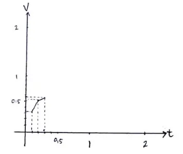
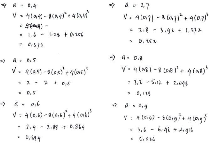
In the process stage, S4 internalized the action by determining the size of the piece by specifying the piece
[image:6.595.333.511.426.576.2]value as a, as in Figure 9. S4 specified the value of a from 0.1 meters, 0.2 meters and 0.3 meters, then substituted it into the equation volume (V = 4a – 8a2 + 4a3). From the coordinates of the values a and the resulting volume, S4 passed through the object stage by encapsulating the process that had been done by coordinating the quantities that had been obtained into a graphic image, which showed the relationship between the size of the piece (a) and the volume of the tank (V) as shown in Figure 10.
Figure 9. S4 substituted the value of the piece to the volume equation
Figure 10. S4 connected h and V quantities with the graph
Text translations: Each piece has the same size, namely
a × a meters. Then the length of each side after being cut is reduced by 2a. Water tank volume = beam volume. V = l ×
w × h = (2 – 2a) (2 – 2a) a. ↓
From the process that had been done, S4 concluded that the larger the size of the piece (a) the greater the volume produced. That S4 summarized it from the graph he produced. This can be seen from the researcher interview transcript with S4 by showing the answer sheet again.
Int.: What can you conclude from the process or image that you produced?
[image:6.595.63.284.597.712.2]0.512, when the value of a is equal to 0.3, the volume is 0.588. I conclude that the greater the value of a, the greater the volume too. This is also seen from this graph [pointing to Figure 10].
Int.: Are you sure about that? What about the other values of a?
S4: hmmm ... [recalculating another a value]
In the next stage, S4 de-encapsulated to determine the value of a which had not been previously assumed, namely 0.4 meters, 0.5 meters, 0.6 meters, 0.7 meters, 0.8 meters, and 0.9 meters. So the value of each tank volume produced based on the size of the piece (a) can be seen in Figure 11. From this result, S4 returned to the object stage which was to reproduce the new graph as shown on Figure 12.
Figure 11. S4 de-encapsulated by substituting other a values
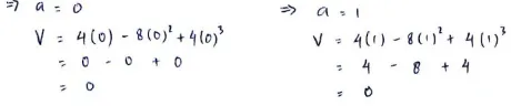
[image:7.595.134.471.177.718.2] [image:7.595.132.467.182.410.2]In the scheme stage, S4 did the same thing as what had been done by S1, which was to re-examine the stages that had been carried out starting from the stages of action, process, and object. On this occasion, S4 was also asked about the volume of the tank before being cut (a = 0 meters) and after being cut to a size of one-meter pieces. After producing a volume with a = 0 meters and a = 1 meters, S4 refined the graph as shown in Figure 12. The following are excerpts of the interview.
Int.: If for example it hasn't been cut, why is the volume like that?
S4: Before being cut, the a is the same as zero, sir. Then the volume is zero [after counting in Figure 13].
Int.: Then if you cut each one in the middle of a sheet of metal, how much is the volume?
S4: He coincides, sir, if it is squeezed, the volume is zero because there is no space. The cut in the middle means that the number of pieces is one, meaning that a is equal to 1 [while subsidizing a = 1 into the volume equation, as shown in Figure 13].
Int.: Oh what can you conclude from the graph?
S4: Oooh, it turns out that even though the pieces are large, it does not necessarily have a large volume, sir.
Figure 13. S4 determined the volume for sizes a = 0 meters and a = 1 meters
4. Discussion
From the results of the study in the form of work results and citation of task-based interviews with the subjects, the researcher described and interpreted the results of the analysis that had been done to show the process of quantitative inductive reasoning and the process of quantitative deductive reasoning. The stages of quantitative reasoning process shown by both subjects (S1 and S4) in solving the problem of covariation are in accordance to the abilities that must be possessed by the subjects in solving problems in quantitative reasoning [4]. When reading and understanding the information of the problem given, S1 and S4 really understood the problem and field shape transformation by writing their interpretations. The subject interpreted quantitative information by identifying the quantities involved in the problem, for example writing the quantity of length, width, height, and volume from the transformation of a flat shape to a beam and believing that the length of the side of the tank is equal to its width because it comes from a square plane. After writing down the quantities involved, the subject planed problem solving using arithmetic and algebra methods. S1 chose to solve the problem with
arithmetic methods using the applicable formula or formula, while S4 used the algebraic method by creating a new symbol in the form of a mathematical model. After the process had been carried out, S1 and S4 both used geometry methods to estimate and check the feasibility of the process, so that it could be the basis for communicating quantitative information verbally and making decisions about the methods they use in solving problems.
The ability of those two subjects in the quantitative reasoning process to solve the problem of covariation shows a different process of thinking. This thinking process was elaborated and reviewed from the stages of the APOS (actions, processes, objects, and schemes). In the
action stage, S1 began by determining the quantity changes that occured by registering or writing down the possibilities of the appropriate value quantities. This value was the basis for determining the quantity of the side of the beam. In this case S1 distinguished it from the long and wide sides (The subject realized that the length was the same as the width, only the length and width to distinguish the two sides of the beam). In determining the value of a long quantity, S1 continuously used the same scale for each change value. Then for a value of wide quantity, he produced a value that was equal to the length quantity because basically the field is square. Changes in long quantities had a direct effect on wide quantities simultaneously. This was reinforced from the results of his research Johnson [9] who said that changing one quantity causes one to simultaneously pay attention to variations in changes in the quantity of another. The stages of this action are S1 subject solves the problem of covariation with direct processes, without making involved quantities into other mathematical forms or equations. In his Johnson [9] study, students compared the quantity of covariations by paying close attention to the numerical values that exist.
In contrast to the thinking process shown by S1, at the action stage, S4 thought by specifying the quantities
involved as variable. This was in accordance to Zeljić [21] statement stating that the iconic model of an object can be seen as a model by understanding variables as objects concretely. In this case S4 used variable a to form a model or equation of the existing quantity (for example, l = 2 – 2a;
w = 2 – 2a; and V = 4a – 8a2 + 4a3). The process carried out by S4 was in accordance to the statement of Moore & Carlson [22] in their research stating that students create formulas to model the relationship between quantity values before performing numerical calculations.
[image:8.595.58.288.370.418.2]predictions about the type of graph, conception of attributes shown by the graph, and differences in language to variations in change and interpretation of the graph [24]. To determine good quantity coordination in drawing graphs covariation problems required many coordination points, but not all students can necessarily interpret them well. These obstacles were stated by Carlson et al. [25] who say that individuals seem to have difficulty forming images (graphs) with a continuous level of change and cannot definitively interpret turning points for dynamic function situations.
5. Conclusions
The quantitative reasoning process on problem solving covariations consists of an inductive quantitative reasoning process (IQRP) and a deductive quantitative reasoning process (DQRP). The IQRP occurs at the action stage, where the process of connecting quantities is carried out directly. The quantities that have been identified are then substituted directly into the applicable formula without making a model or mathematical equation. While the DQRP occurs at the action stage, where the process of connecting quantity is done by making mathematical modeling or equations. The modeling or equation is based on the example performed by specifying the quantities involved in the problem of covariation as a variable. Furthermore, the stages of the process, object, and scheme of IQRP and DQRP are carried out in almost the same way namely to determine the relationship of quantity of covariation. It is done by substituting values into mathematical formulas or equations and then illustrated in a graph of coordination of quantities.
This study shows that students understand situations that occur from covariate quantity relationships and then understand the process (reasoning) about how the values of quantity change together. This study also provides information about student reasoning when understanding problems that change together and is useful for curriculum design and learning to pay attention to the nature of the problem context and encourage students to think about the quantity relationship in solving problems. Learning must also support students in reflecting on the context of the problem as a way for them to re-examine the problem solving that has been produced and correct the wrong solution.
REFERENCES
NCTM., 2000. Principle and Standards for Schools [1]
Mathematics. Resto, VA.
P. W. Thompson. Quantitative reasoning, complexity, and [2]
additive structures. Educational studies in Mathematics,
25(3), 165-208, 1993.
E. Weber, A. Ellis, T. Kulow, & Z. Ozgur. Six principles for [3]
quantitative reasoning and modeling. Mathematics Teacher, 108(1), 24-30, 2014.
C. A. Dwyer, A. Gallagher, J. Levin, & M. E. Morley. What [4]
is quantitative reasoning? Defining the construct for assessment purposes. ETS Research Report Series, 2003(2), 2003.
National Governors Association (NGA) Center for Best [5]
Practices & Council of Chief State School Officers. (2010). Common Core State Standards for Mathematics. Washington D.C.
M. P. Carlson, B. Madison, & R. D. West. A study of [6]
students’ readiness to learn calculus. International Journal of Research in Undergraduate Mathematics Education, 1(2), 209-233, 2015.
H. E. Stalvey, & D. Vidakovic. Students’ reasoning about [7]
relationships between variables in a real-world problem. The Journal of Mathematical Behavior, 40, 192-210, 2015. S. Yemen-Karpuzcu, F. Ulusoy, & M. Işıksal-Bostan. [8]
Prospective Middle School Mathematics Teachers’ Covariational Reasoning for Interpreting Dynamic Events during Peer Interactions. International Journal of Science and Mathematics Education, 15(1), 89-108, 2017. H. L. Johnson. Reasoning about variation in the intensity of [9]
change in covarying quantities involved in rate of change. The Journal of Mathematical Behavior, 31(3), 313-330, 2012.
H. L. Johnson. Secondary students’ quantification of ratio [10]
and rate: A framework for reasoning about change in covarying quantities. Mathematical Thinking and Learning, 17(1), 64-90, 2015.
E. Dubinsky. Reflective Abstraction in Advanced [11]
Mathematical Thinking. Advanced Mathematical Thinking, 95–126, 2002.
I. Arnon, J. Cottrill, E. Dubinksy, A. Oktaҫ, S. R. Fuentes, M. [12]
Trigueros, & K. Weller. APOS theory: A framework for research and curriculum development in mathematics education. Berlin. Springer, 2014.
A. Maharaj. An APOS analysis of natural science students’ [13]
understanding of integration. Journal of Research in Mathematics Education, 3(1), 54-73, 2014.
A. Burns-Childers, & D. Vidakovic. Calculus students’ [14]
understanding of the vertex of the quadratic function in relation to the concept of derivative. International Journal of Mathematical Education in Science and Technology, 49(5), 660-679, 2017.
V. Borji, H. Alamolhodaei, & F. Radmehr. Application of [15]
the APOS-ACE Theory to improve Students’ Graphical Understanding of Derivative. Eurasia Journal of Mathematics, Science and Technology Education, 14(7), 2947-2967, 2018.
L. García-Martínez, & M. Parraguez. The basis step in the [16]
E. Tokgoz. Analysis of STEM Majors’ Calculus Knowledge [17]
by Using APOS Theory on a Quotient Function Graphing Problem. In ASEE Annual Conference Proceedings, paper ID (Vol. 12664), 2015.
M. B. Miles, A. M. Huberman, & J. Saldana. Qualitative [18]
Data Analysis: A Methods Sourcebook (Third edition). Sage, London, 2014.
Shell Centre for Mathematical Education (University of [19]
Nottingham). The language of functions and graphs: An examination module for secondary schools: Nottingham, UK: JMB/Shell Centre for Mathematical Education, 1985. J. Corbin, & A. Strauss. Basics of qualitative research: [20]
Techniques and procedures for developing grounded theory (3rd ed.). London: Sage Publications, 2008.
M. Zeljić. Modelling the Relationships between Quantities: [21]
Meaning in Literal Expressions. Eurasia Journal of Mathematics, Science & Technology Education, 11(2), 431-442, 2015.
K. C. Moore, & M. P. Carlson. Students’ images of problem [22]
contexts when solving applied problems. The Journal of Mathematical Behavior, 31(1), 48-59, 2012.
H. L. Johnson, & E. McClintock. A link between students’ [23]
discernment of variation in unidirectional change and their use of quantitative variational reasoning. Educational Studies in Mathematics, 1-18, 2018.
K. C. Moore, & P. W. Thompson. Shape thinking and [24]
students’ graphing activity. In T. FukawaConnelly (Ed.), Proceedings of the 18th Meeting of the MAA Special Interest Group on Research in Undergraduate Mathematics Education (pp. 782–789). Pittsburgh, PA: RUME, 2015. M. P. Carlson, S. Jacobs, E. Coe, S. Larsen, & E. Hsu. [25]