Graph kernels and applications in protein classification

Journal of Chemical and Pharmaceutical Research, 2014, 6(2):563-569

Research Article

_{CODEN(USA) : JCPRC5}

ISSN : 0975-7384

Graph kernels and applications in protein classification

Jiang Qiangrong*, Xiong Zhikang and Zhai Can

Beijing University of Technology, Department of Computer Science, Beijing, China

_____________________________________________________________________________________________

ABSTRACT

Protein classification is a well established research field concerned with the discovery of molecule’s properties through informational techniques. Graph-based kernels provide a nice framework combining machine learning techniques with graph theory. In this paper we introduce a novel graph kernel method for annotating functional residues in protein structures. A structure¬ is first modeled as a protein contact graph, where nodes correspond to residues and edges connect spatially neighboring residues. In experiments on classification of graph models of pro-teins, the method based on Weisfeiler Lehman shortest path kernel with complement graphs outperformed other state-of-art methods.

Keywords: Protein classification, Machine learning, Graph kernels, Shortest path, Weisfeiler-Lehman.

_____________________________________________________________________________________________

INTRODUCTION

Kernel methods are an important method which is widely used in statistical learning theory[1]. Kernels help to adapt classification regardless how classification performs. That is to say, kernels act like an interface between clas-sification tools and data sets via Support Vector Machines[2]. Early studies on kernel methods dealt almost exclu-sively with vector-based descriptions of input data. This procedure, though convenient, does not always effectively capture topological relationships inherent to the data; therefore, the power of the learning process may be insuffi-cient. Haussler[3] was the first to define a principled way of designing kernels on structured objects, the so-called R-convolution kernel. Over recent years, kernels on structured objects such as strings and trees[4], on nodes in graphs and on graphs have been defined. Graphs are natural data structures to model such structures, with nodes representing objects and edges the relations between them[5]. In this context, one often encounters two questions: “How similar are two nodes or edges in a given graph?” and “How similar are two graphs to each other?”

[image:2.595.95.522.72.192.2]

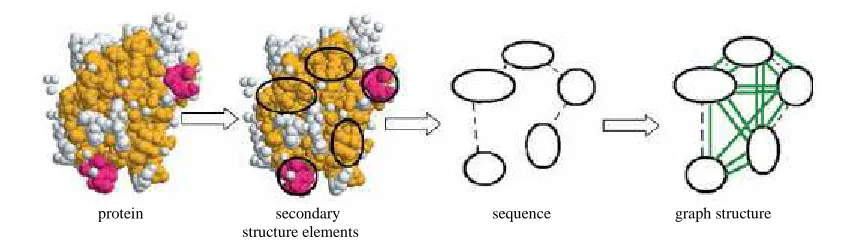
protein secondary sequence graph structure structure elements

Fig. 1: Illustration of graph generation from PDB protein file

EXPERIMENTAL SECTION

2.1 Some Definitions on Graph Theory

We define a graph G as a triplet

(

V

,

E

,

l

)

, where

V

is the set of vertices,

E

is the set of undirected edges, and

∑

→

V

l :

_{is a function that assigns labels from an alphabet}

∑

to nodes in the graph. The neighborhood

Ν

(v

)

of

a node

v

is the set of nodes to which

v

is connected by an edge, that is

Ν

(

v

)

=

{

v

'

(

v

,

v

'

)

∈

E

}

. We assume that

every graph has

n

nodes,

m

_{edges, and a maximum degree of}

d

.

The adjacency matrix

A

of

G

is defined as follows:

[ ]

,

0

,

)

,

(

1







_∈

=

otherwise

E

v

v

if

A

_ij i j

where

v

_i and

v

_j are nodes in

G

. Labels can be added on nodes or edges, these labels are referred as attributes.

A walk

w

of length

k

−

1

in a graph is a sequence of nodes

v

₁

,

v

₂

,

⋅

⋅⋅

,

v

_k where

(

v

_i−1

,

v

_i

)

∈

E

for

1

<

i

≤

k

.

A path

p

is a walk without same nodes in the sequence.

A cycle is a walk with

v

1

=

v

_k,a simple cycle does not have any repeated nodes except for

v

1.

Suppose

G

(

V

,

E

)

is a graph with vertex set

V

and edge set

E

. Then, its complement

G

(

V

,

E

)

is a graph with the

same vertex set

V

, but with a different edge set

E

=

V

×

V

\

E

. In other words, the complement graph is made up of all the edges missing from the original graph.

2.2 Graph Isomorphism

Graph similarity or isomorphism[13] is the most essential problem for learning tasks like clustering and classifica-tion on graphs. In graph theory, an isomorphism of graphs

G

and

H

is a bijection between the vertex sets of

G

and

H

:

f

:

V

(

G

)

→

V

(

H

)

, such that any two vertices

u

and

v

of

G

are adjacent in

G

if and only if

f

(u

)

and

f

(v

)

are adjacent in

H

. Graph isomorphism problem is neither known to be polynomial-computable, nor NP-hard[14].

2.3 The Weisfeiler-Lehman Test of Isomorphism

Our method uses concepts from the Weisfeiler-Lehman test of isomorphism[15][16], more specifically its 1-dimensional variant. Assume we are given two graphs

G

and

H

and we would like to test whether they are iso-morphic. The 1-dim Weisfeiler-Lehman test proceeds in iterations, which we index by

i

and which comprise the steps given in Algorithm 1.

The key idea of the algorithm is to augment the node labels by the sorted set of node labels of neighboring nodes, and compress these augmented labels into new, short labels. These steps are then repeated until the node label sets of

G

and

H

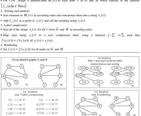
are isomorphic, or the algorithm has not been able to determine that they are not isomorphic. See Fig 2, for an illustration of these steps.

Algorithm 1. One iteration of the 1-dim. Weisfeiler-Lehman test of graph isomorphism(1968)

1. Multiset-label determination

For

i

=

0

,set

M

_i

(

v

)

=

l

₀

(

v

)

.

For

i

>

0

, assign a multiset-label

M

_i

(v

)

to each node

v

in

G

and

H

which consists of the multiset

{

l

_i−1

(

u

)

u

∈

Ν

(

u

)

}

. 2. Sorting each multiset

Sort elements in

M

i

(v

)

in ascending order and concatenate them into a string

s

i

(v

)

.

Add

l

i−1

(

v

)

as a prefix to

s

i

(v

)

and call the resulting string

s

i

(v

)

.

3. Label compression

Sort all of the strings

s

_i

(v

)

for all

v

from

G

and

H

in ascending order.

Map each string

s

i

(v

)

to a new compressed label, using a function

∑

→

∑

*

:

f

such that

))

(

(

))

(

(

s

v

f

s

w

f

i

=

i iff

s

i

(

v

)

=

s

i

(

w

)

.

4. Relabeling

Set

l

i

(

v

)

=

f

(

s

i

(

v

))

for all nodes in

G

and

H

.

[image:3.595.70.545.161.550.2]

Fig. 2: Illustration of the 4 steps of one iteration of the computation of the Weisfeiler-Lehman test of isomorphism

2.4 Weisfeiler-Lehman Sequence Graphs

Define the Weisfeiler-Lehman graph at height

i

of the graph

G

=

(

V

,

E

,

l

)

as the graph

G

_i

=

(

V

,

E

,

l

_i

)

. We call

the sequence of Weisfeiler-Lehman graphs,

)},

,

,

(

,

),

,

,

(

),

,

,

{(

}

,

,

,

{

G

0

G

1

⋅

⋅⋅

G

h

=

V

E

l

0

V

E

l

1

⋅

⋅⋅

V

E

l

h

where

G

0

=

G

, the Weisfeiler-Lehman sequence up to height

h

of

G

.

G

0 is the original graph,

G

1

=

r

(

G

0

)

is the graph resulting from the first relabeling, and so on.

2.5 Weisfeiler-Lehman Kernel with Complement Graphs

Let

k

be any kernel for graphs, that we will call the base kernel. Then the Weisfeiler-Lehman kernel with

h

).

,

(

)

,

(

)

,

(

)

,

(

_{0 0 1 1 h h}

h

WL

G

H

k

G

H

k

G

H

k

G

H

k

=

+

+

⋅

⋅⋅

+

If we take the complement graphs into consideration, we will derive the Weisfeiler-Lehman kernel with comple-ment graphs:

+

+

+

=

(

,

)

(

,

)

(

,

)

)

,

(

G

H

k

G

0

H

0

k

G

0

H

0

k

G

1

H

1

k

wlh

k

(

G

1

,

H

1

)

+

⋅

⋅⋅

+

k

(

G

h

,

H

h

)

+

k

(

G

h

,

H

h

),

where

(

G

₀

,

G

₁

,

⋅

⋅⋅

,

G

_h

),

(

H

₀

,

H

₁

,

⋅

⋅⋅

,

H

_h

)

are complement graphs of

(

G

0

,

G

1

,

⋅

⋅⋅

,

G

h

),

(

H

0

,

H

1

,

⋅

⋅⋅

,

H

h

).

Let the base kernel

k

be any positive semidefinite kernel on graphs. Then the corresponding Weisfeiler-Lehman

kernel

k

_WLh is positive semidefinite.

2.6 Shortest Path and Floyd-Warshall Algorithm

Given an undirected graph

G

=

(

V

,

E

)

the shortest path graph[17],

G

sp

(

V

,

E

'

)

, which contains the same set of

vertices as

G

and the edge between every pair of vertices is labeled with the shortest distance between them in the

original graph. The transformation from

G

to

G

_spcan be performed by any all-pairs shortest path algorithm.

Floyd–Warshall algorithm(See Algorithm 2)[18] is attractive and effective because it is straightforward and has time

complexity of

O

(

n

3

)

. Then, a kernel function was used to calculate the similarity between two shortest path graphs according to the following definitions, which were first defined by Borgwardt and Kriegel[9]. It is proved to be a positive semidefinite kernel and is computable in polynomial time.

Algorithm 2. Floyd–Warshall algorithm (Graph

G

with

n

nodes and adjacency matrix

A

) Floyd(

G

)

for

k

←

1

to

n

for

i

←

1

to

n

for

j

←

1

to

n

if(cost(

i,

k

)+cost(

k,

j

)<cost(

i,

j

))

cost(

i,

j

)=cost(

i,

k

)+cost(

k,

j

) endif

endfor endfor endfor

Let

e

₁be the edge connecting vertices

v

₁ and

w

₁ on graph

G

, and

e

₂be the edge connecting nodes

v

₂ and

w

₂

on graph

H

. A walk on an edge includes the edge and its two adjacent vertices. A walk kernel

k

_walkis used to

compare the walk

e

₁and

e

₂as:

k

_walk

(

e

₁

,

e

₂

)

=

k

_node

(

v

₁

,

v

₂

)

*

k

_edge

(

e

₁

,

e

₂

)

*

k

_node

(

w

₁

,

w

₂

)

,

where

k

node is the kernel

function for comparing two vertices, and

k

_edge

is a kernel function forcomparing two edges.

The kernel function for comparing two vertices

u

and

v

is a Gaussian kernel[19] over their respective feature vec-tors,

.

2

)

(

)

(

exp

)

,

(

2 2

















₋

=

δ

v

f

u

f

v

u

k

_node

The kernel function for comparing two edges

e

and

f

is a Brownian bridge kernel that assigns the highest value to edges with identical weights, and 0 to all edges that differ in weight more than a constant

c

:

).

)

(

)

(

,

0

max(

)

,

(

e

f

c

length

e

length

f

2.7 Shortest Path Kernel

Given two shortest path graphs

G

(

V

₁

,

E

₁

)

and

H

(

V

₂

,

E

₂

)

the shortest path graph kernel:

),

,

(

)

,

(

_{1 2}

1 1 2 2

e

e

k

H

G

k

E e e E

walk

sp

∑ ∑

∈ ∈

=

where

k

_walk is a kernel function for comparing two edge walks of length 1.

Floyd-transformation requires

O

(

n

3

)

time.

E

₁ and

E

₂contain

O

(

n

2

)

edges. The computation of the

shortest-path graph kernel requires

O

(

n

4

)

time.

2.8 Weisfeiler-Lehman Shortest Path Kernel with Complement Graphs

With the above definitions, we are ready to define Weisfeiler-Lehman shortest path kernel with complement graphs as:

.

)

,

(

)

,

(

)

,

(

)

,

(

)

,

(

)

,

(

)

,

(

1 1 1 1 0 0 0 0 h h sp h h sp sp sp sp sp h WL

H

G

k

H

G

k

H

G

k

H

G

k

H

G

k

H

G

k

H

G

sp

k

+

+

⋅⋅

⋅

+

+

+

+

=

For

N

graphs, the runtime of WL shortest path kernel will scale as

O

(

N

2

n

4

)

.

RESULTS AND DISCUSSION

We compared the performance of the random walk graph kernel[20], the shortest path kernel, the WL Shortest Ker-nel without complement graphs and WL Shortest KerKer-nel with complement graphs in terms of classification accuracy of the classification on D&D[21] and ENZYMES datasets, where accuracy shows the overall percentage of correct classifications. D&D is a dataset of 691 enzymes and 487 non-enzymes. Each protein is represented by a graph, in which the nodes are amino acids and two nodes are connected by an edge if they are less than 6 Ångstroms apart. The task is to classify the protein structures into enzymes and non-enzymes. ENZYMES is a data set of protein ter-tiary structures obtained from Borgwardt et al(2005), consisting of 600 enzymes from the BRENDA enzyme data-base(Schomburget al., 2004). In this case the task is to correctly assign each enzyme to one of the 6 EC top-level classes. Nodes are labeled in the dataset. In terms of D&D, we also analyzed the sensitivity, specificity, and Mat-thews correlation coefficient (MCC)[22] of the classifications in addition to accuracy (Table 3), where sensitivity is the percentage of enzymes that have been correctly classified as enzymes , specificity indicates the percentage of non-enzymes that have been correctly classified, and MCC shows the overlapping between the predictions and the actual distribution.

Suppose P represents positive instances N negative instances, TP the number of true positives, TN the number of true negatives, FP the number of false positives and FN the number of false negatives. Then the accuracy, sensitivi-ty, specificity and MCC can be calculated by the following formulas,

N

P

TN

TP

accuracy

+

+

=

,

FN

TP

TP

P

TP

y

sensitivit

+

=

=

,

TN

FP

TN

N

TN

y

specificit

+

=

=

,

.

)

)(

)(

)(

(

TP

FP

TP

FN

TN

FP

TN

FN

FN

FP

TN

TP

MCC

+

+

+

+

×

−

×

=

[image:6.595.79.542.90.142.2]

Table 1: The classification accuracy(%) and standard deviation of each kernel on protein data sets

[image:6.595.70.542.169.258.2]

Method/Data set D&D ENZYMES Random Walk Kernel 70.26(±0.86) 20.14(±0.69) Shortest Path Kernel 78.19(±0.26) 42.18(±0.43) WL Shortest Path Kernel without complement graphs 81.27(±0.70) 62.47(±0.61) WL Shortest Path Kernel with complement graphs 83.64(±0.92) 63.96(±0.84)

Table 2: CPU runtime for kernel computation on protein classification

Data set D&D ENZYMES Class size 2 6 Maximum nodes 5478 126 Average nodes 284.32 32.63

Number of graphs 1178 600 Random Walk Kernel 52days 39days Shortest Path Kernel 25h 17min22s 38s WL Shortest Path Kernel without complement graphs 64days 1min3s WL Shortest Path Kernel with complement graphs 71days 2min11s

Table 3: Comparison of our method with others using D&D data set

Method Sensitivity Specificity MCC Random Walk Kernel 65.28% 71.35% 0.523 Shortest Path Kernel 71.32% 79.64% 0.736 WL Shortest Path Kernel without complement graphs 78.24% 83.77% 0.821 WL Shortest Path Kernel with complement graphs 81.05% 86.13% 0.836

In terms of runtime, The shortest path kernel and the WL shortest path kernel were competitive to the random walk kernel on smaller graphs (ENZYMES), but on D&D their runtime degenerated to more than 25 hours for the shortest path kernel, 64 days for the WL shortest path kernel without complement graphs and 71 days for the WL shortest path kernel with complement graphs. Using a graph to model the distribution of amino acid residues on the 3D structure, our method efficiently captures various structural determinants related to protein function. The kernels using WL method performed better than other kernel types. Furthermore, the WL shortest path kernel with comple-ment graphs outperforms the other kernels with an accuracy of at least 83.64%, and it achieves improvecomple-ments in accuracy more than 2% over the WL shortest path kernel without complement graphs. Meanwhile, considering shortest paths instead of walks increases classification accuracy significantly. For the random walk kernel, classifi-cation is the worst as with an increasing number of tottering walks, classificlassifi-cation accuracy decreases. Table 3 also shows that our proposed method outperforms other methods.

CONCLUSION

In this paper, we propose a simple yet effective and efficient graph classification approach that is based on topolog-ical and label graph attributes. Our main idea is that graphs from the same class should have similar attribute values. On the basis of an extensive comparison with state-of-the-art graph kernel classifiers, we show that our approach yields competitive or better accuracies and has typically much lower computational times. Our conclusion is that graph attributes are effective in capturing discriminating structural information from different classes. Our new ker-nels based on Weisfeiler-Lehman test of isomorphism open the door to applications of graph kerker-nels on large graphs in bioinformatics, for instance, protein function prediction via detailed graph models of protein structure on the ami-no acid level, or on gene networks for pheami-notype prediction. A challenging question for further studies will be to consider kernels on graphs with continuous or high-dimensional node labels and their efficient computation.

Acknowledgments

This project is supported by Beijing Municipal Education Commission. The authors are grateful to the Beijing Uni-versity of Technology for financial support.

REFERENCES

[1]Vapnik V. The nature of statistical learning theory, Springer-Verlag, New York, 1995.

[2]V.N. Vapnik, S.E. Golowich and A.J. Smola. Adv. Neural Information Procession Syst, 1996, 281-287.

[3]D. Haussler. Convlution kernels on discrete structures, Technical Report, Department of Computer Science, University of California at Santa Cruz, 1999.

[image:6.595.73.542.286.337.2]

[6]H. Xiangguang, W. Yaya and G. Wei. Journal of Chemical and Pharmaceutical Research, 2013, 5(12), 196-200. [7]K.M. Borgwardt et al. BIOINFORMATICS, 2005, 21(1), i47-i56.

[8]J. Ramon and T. Gärtner. Proceedings of the First International Workshop on Mining Graphs, Trees and

Se-quences, 2003, 65-74.

[9]K.M. Borgwardt and H.-P. Kriegel. Proceedings of the Fifth IEEE International Conference on Data Mining,

2005, 74-81.

[10]V. Vacic, M. L. Iakoucheva, S. Lonardi and P. Radivojac. Journal of Computational Biology, 2010, 17(1), 55-72.

[11]N. Shervashidze et al. International Conference on Artificial Intelligence and Statistics, 2009, 488-495. [12]P. Mahé and J.-P. Vert. Machine Learning, 2009, 75(1), 3-35.

[13]D.L.Vertigan and G.P. Whittle. Journal of Combinatorial Theory, Series B, 1997, 71(2), 215–230.

[14]V. N. Zemlyachenko, N. M. Korneenko and R. I. Tyshkevich. Journal of Soviet Mathematics, 1985, 29(4), 1426–1481.

[15]B.J. Weisfeiler and A.A. Leman. Naucho-Technicheskaja Infrormatsia, 1968, 2(9), 12-16.

[16]B.J. Weifeiler. On construction and identification of graphs, Springer-Lecture Notes in Mathematics, New York, 1976.

[17]R.W. Floyd. Communications of the ACM, 1962.

[18]B.V. Cherkassky, A.V. Goldberg and T. Radzik. Mathematical programming, 1996, 73(2), 129-174. [19]J. Wang , H. Lu and K.N. Plataniotis. Pattern recognition, 2009, 42(7), 1237-1247.

[20]H. Kashima, K. Tsuda and A. Inokuchi. Proceedings of the Twentieth International Conference on Machine

Learning, 2003, 321-328.

[21]P.D. Dobson and A.J. Doig. Journal of Molecular Biology, 2003, 330(4), 771-783. [22]D.M.W. Powers. Journal of Machine Learning Technologies, 2011, 2(1), 37-63.