2D Multi Band PCA and its Application for Ear Recognition

Citation:

Zarachoff, M and Sheikh Akbari, A and Monekosso, D (2018) 2D Multi-Band PCA and its Application

for Ear Recognition. In: 2018 IEEE International Conference on Imaging Systems and Techniques

(IST). IEEE. ISBN 978-1-5386-6628-9 DOI: https://doi.org/10.1109/IST.2018.8577132

Link to Leeds Beckett Repository record:

http://eprints.leedsbeckett.ac.uk/5284/

Document Version:

Book Section

Conference paper

The aim of the Leeds Beckett Repository is to provide open access to our research, as required by

funder policies and permitted by publishers and copyright law.

The Leeds Beckett repository holds a wide range of publications, each of which has been

checked for copyright and the relevant embargo period has been applied by the Research Services

team.

We operate on a standard take-down policy.

If you are the author or publisher of an output

and you would like it removed from the repository, please

contact us

and we will investigate on a

case-by-case basis.

XXX-X-XXXX-XXXX-X/XX/$XX.00 ©20XX IEEE

2D Multi-Band PCA and its Application for Ear

Recognition

Matthew Zarachoff

School of Computing, Creative Technologies & Engineering

Leeds Beckett University Leeds, United Kingdom

m.zarachoff4868 @student.leedsbeckett.ac.uk

Akbar Sheikh-Akbari

School of Computing, Creative Technologies & Engineering

Leeds Beckett University Leeds, United Kingdom [email protected]

Dorothy Monekosso

School of Computing, Creative Technologies & Engineering

Leeds Beckett University Leeds, United Kingdom [email protected]

Abstract—Principal Component Analysis (PCA) has been successfully used for many application including ear recognition. However, its performance is limited due to its significant data dependency. This paper presents a two dimensional multi-band PCA (2D-MBPCA) method, which has shown a significantly higher performance to that of the PCA. The proposed method divided the input gray image into a number of images, based on the intensity of its pixels using either a dynamic or predefined equal rang thresholds’ values. PCA is then applied on the resulting set of images to extract their features. The resulting features are used to find the best match. The application of the proposed 2D-MBPCA for ear recognition using two benchmark ear image datasets, shows the merit of the proposed technique to that of the standard PCA.

Keywords—PCA, ear recognition, histogram equalization.

I. INTRODUCTION

Ear recognition is a field in biometrics wherein images of the ears are used to identify individuals. Ears are unique to an individual, so much so that identical twins can have differentiable ears [1]. Much research has been done in the last two decades regarding ear recognition concerning both the feature extraction and comparison of features of ear images [2-6]. Principal Component Analysis (PCA) has been used extensively in ear recognition for both feature extraction [2-4] and feature reduction to reduce dimensionality of the data [5-6]. Over the last two decades, researchers have proposed different methods to improve the performance of PCA on feature extraction. They showed that the extended PCA methods could improve overall performance over the standard PCA, in terms of computation costs, dimensionality reduction, memory usage and performance [9-11] (extended PCA based method are reviewed in Section II). However, in author’s knowledge, no extension of PCA method for single image feature extraction have been reported in the literature. This has inspired us to propose our two dimensional multi-band PCA (2D-MBPCA) for ear recognition approach.

This paper presents a two dimensional multi-band PCA (2D-MBPCA) method for ear recognition. The proposed technique splits the input image into a number of images with different gray level pixel values. Two methods are investigated

for dividing the input image pixels into different images. In the first method, the full gray scale equally is divided between the target numbers of the images. In the second approach, an iterative divide and test approach based on the hill climbing optimization method is used to divide the input image pixels into the target images. The proposed algorithm then applies the standard PCA method on the resulting set of images, extracting their principal components as their features. These features are used for ear recognition. Experimental results on the images of two benchmark ear image datasets demonstrates that the proposed 2D-MBPCA technique greatly outperforms PCA based matching algorithm on the original images. The rest of the paper is organized as follows: Section II gives a brief background of the ear recognition problem and current solutions, Section III introduces the proposed technique, Section IV describes the experimental results, and Section V concludes the paper.

II. BACKGROUND

A. Ear Recognition

Much research has been conducted in the field of ear recognition [2-6]. Ear recognition techniques can be classified into several categories, including holistic and hybrid methods. Principal Component Analysis (PCA) and other related methods are examples of holistic techniques. These techniques extract some features from the ear image and use it as a basis for recognition. The first use of PCA for biometrics was reported by Turk and Pentland in [7] and demonstrated the use of PCA on images of faces to perform facial recognition in a technique called “eigenfaces”. This process uses a training set to calculate the eigenvectors that span the “eigenface” space and then project facial images into that space. The resulting projections are then compared using nearest neighbor critoria. Victor, Bowyer, and Sarkar [2] later applied this method to ear and face images. They reported that facial recognition gives higher accuracy matching than that of the ear recognition, however, ears still demonstrates merit. A similar experiment was later conducted by Chang, Bowyer, Sarkar, and Victor [3] on both face and ear images. They concluded that the difference in accuracy between ear and facial image recognition is not statistically significant, however both are

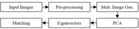
Fig. 1. Two dimensional multi-band PCA (2D-MBPCA) method Pipeline.

useful biometrics. PCA in conjunction with other techniques has also been used for ear recognition. Nosrati, Faez, and Faradji were used the application of the PCA on 2D wavelet coefficients of the ear images for ear recognition in [8]. They applied PCA on the summation of wavelet high-frequency subbands’ coefficients and used the resulting eigenvectors for matching. They reported superior performance to those of the PCA and ICA methods.

B. Application of PCA for Hyperspectral Image Processing Hyperspectral images are images that are taken across multiple bands within the electromagnetic spectrum. The set of images captured by hyperspectral sensors can considered as a data cube with coordinates (x, y, λ), where x and y correspond to 2D positions and λ is the individual wavelength for a given slice. PCA and other dimensionality reduction techniques have been extensively investigated for feature extraction from hyperspectral images [9-11]. Harsanyi and Chang introduced a technique for hyperspectral image classification and dimensionality reduction in [9]. They solved the eigenvector problem in a similar manner to PCA, while simultaneously allowing for classification during feature reduction. Various extensions of PCA for hyperspectral images have also been reported in the literature [10-11]. Jia and Richards proposed the Segmented-PCA for hyperspectral image classification in [10]. Their technique divides the input hyperspectral images into a number of groups based on the correlations amongst the images. The PCA is then applied individually on images within each bands. The extracted features are finally used for image classification. Zabalza et al. in [11] proposed a Folded-PCA method for hyperspectral image classification. In Folded-PCA each spectral vector is transformed into a matrix, based on which, a partial covariance matrix can be directly determined and then accumulated for Eigen decomposition and data projection. They showed that the performance of the Folded-PCA is a function of the number of the groups used to split the spectral in it, as it affects how much additional information can be extracted for added-value to the conventional PCA. Results show that Folded-PCA outperforms conventional PCA and segmented-PCA, with respect to classification accuracy.

III. PROPOSED 2DMULTIBAND PCATECHNIQUE

Let E be the set of all ear images where each image in E is of size x × y. Each image e ϵ E is subjected to four steps: A) Image pre-processing, B) Multiple-image generation, C) PCA, and D) Image matching. The overall process is illustrated in Fig. 1.

A. Image Pre-processing

The images in E are pre-processed as follows: First, map the pixel intensities so they lie in the range of [0,1]. The

resulting images are then subject to histogram equalization to increase their contrast. Histogram equalization is performed through the following steps:

• Calculate the Probability Mass Function (PMF) of the image from its histogram

• Use the PMF to calculate the Cumulative Distribution Function (CDF)

• Map each pixel’s intensity to a new gray level value using the CDF

After histogram equalization, each of the image in E is ready to be converted into multiple images.

B. Multiple-Image Generation

Let N be the number of partitions desired for the image e and let b = [b1, b2, …, bN-1] be the division along which to split

e into. Then the image e is split into multiple images as follows:

• Generate N images of size x × y, called F = [f1, f2, …,

fN] with all pixel values equal to zero.

• For each pixel p of intensity [0, b1) in e, assign the same

pixel value to its respective pixel in image f1.

• Repeat the process for [b2, b3), [b3, b4), …[bN-1,1] for

image f2, …, fN..

The result is that each image e is now a collection of images F. Each F can be considered to be a sort of a hyperspectral image, where each f ϵ F captures its own intensity band. An illustration of this process is presented in Fig. 2, and an example of a F image is shown in Fig. 3.

Fig. 2. The Multiple Image Generation Process

C. Principal Component Analysis (PCA)

For each image f ϵ F, a mean adjusted image f’ can be created as follows:

f’ = f – fM (1)

where fM is the mean value of all of the pixels in f. If each

image f’ is converted to a column wise vector of length (x×y), the bin-set of e can be represented as a matrix B of size (x×y) × N. PCA is performed using Singular Value Decomposition (SVD) on B to create the following decomposition:

B = UΣVT ₍₂₎

where U is of size (x×y) × (x×y), Σ is of size (x×y) × N-1, and VT _{is of size N-1 × N-1. The columns of V are then the}

orthonormal eigenvectors of the covariance matrix of B and Σ is a diagonal matrix of the eigenvalues of the covariance matrix of B. The eigenvectors form a basis for an eigenspace for each image. The components in V are then used for matching.

D. Image Matching

Let U = u1, u2…, uN-1 be the set of principal components of

some query image q. Let r be an image in the dataset of images R with principal components V = v1, v2, …vN-1. The set of

Euclidean distances D = d1, d2,…, dN-1 between q and r is then

shown in equation 3:

dn = (sum(un – vn)2)1/2 (3)

After the distances dn are calculated, they are averaged into

a singular distance metric. This singular distance S between q and r is then written in equation 4:

S = sum(D) / (N – 1) (4)

The best match for q in the dataset R is the image for which S is minimized.

IV. EXPERIMENTAL RESULTS

This investigation uses two benchmark image datasets: The Indian Institute of Technology Delhi II (IITD II) dataset [12] and the University of Science and Technology Beijing II (USTB II) dataset [13]. IITD II dataset consists of 793 images of the right ear of 221 participants. Each participant was photographed between three and six times, with each image being of size 180 × 50 pixels and in 8-bit grayscale. For consistency, only the first three images for any individuals are used in this research. The USTB II dataset consists of 308 images of the right ear of 77 participants, each of whom were photographed four times. Unlike IITD II, the images in USTB II are not tightly cropped. The first image for each participant in this dataset is a frontal image under standard illumination condition, the second and the third images are rotated by +30 and -30 degrees respectively, and the fourth image is taken under weak illumination. Examples of images of multiple

subjects from both the IITD II and the USTB II datasets can be seen in Fig. 4.

Three separate experiments were conducted. The first experiment was used to generate a baseline for comparison, the second experiment determined the number of images to be generated and number of the principal components used, and the last experiment was an attempt at dynamically choosing the number of bins and bin size. All experiments were conducted as follows:

• Select the first image of each subject to act as a query set; let the rest of the images serve as a dataset for that image.

• Perform the 2D Multiband PCA Technique on both the query set and dataset images as described in Section III.

• For each query image, if it is correctly matched with a dataset’s image, mark it as a Top-1 image. Similarly, if it is correctly matched with one of the closest five images, mark it as a Top-5 image.

• The percentage of Top-1 and Top-5 images of the dataset are the Top-1 and Top-5 accuracies.

• Repeat this process for the second, third, and in the case of USTB II, fourth images for each individual. Average the Top-1 and Top-5 accuracies across all trials.

TABLE I. BASELINE COMPARISON OF PCA Dataset

Used

Type of Match

Top-1 Top-5

IITD II 36.35% 52.94% USTB II 17.21% 34.09%

A. Experiment to Generate a Baseline

To create a baseline, PCA was applied to each image individually. The resulting eigenvectors were then compared as discussed above. The results for both the IITD II and USTB II datasets are presented in Table I. It can be seen that IITD II’s baseline is higher than USTB II’s. This is likely due to the rotations present in the USTB dataset, making it more challenging.

B. Experiment to Determine the Number of Bins and Principal Components

The proposed method was applied to both datasets using two to 10 partitions. For a set of trials using N partitions, the size of each partition was defined as 1/N, corresponding to an intensity band between zero and one. In this experiment, the number of principal components was varied between one and N-1. The number of correct matches was calculated for each combination of partition count and principal component count. A subset of the results for both the IITD II and USTB II datasets are presented in Tables II through V, with the most accurate trial in bold. The matching accuracy produced this method increased as the number of partitions increased to a point, but then decreased. For brevity, only the results up to and including the maximum accuracy are included in the presented tables.

Results show that the proposed method greatly outperforms the baseline on both the IITD II and USTB II datasets. Furthermore, and an increased number of features used for a given number of bins is correlated with a higher accuracy. The IITD II dataset required fewer partitions to achieve its best accuracy than the USTB II dataset. This is likely due to the increased complexity of the USTB II dataset and the fact that the IITD II dataset is tightly cropped, while the USTB II dataset is not.

TABLE II. TOP-1 ACCURACY FOR THE IITD II DATASET Number of

Bins

Number of Principal Components

1 2 3 4

2 89.29% - - -

3 88.69% 92.61% - -

4 86.27% 90.80% 91.86% - 5 84.31% 88.69% 90.95% 92.76%

TABLE III. TOP-5 ACCURACY FOR THE IITD II DATASET Number of

Bins

Number of Principal Components

1 2 3 4

2 95.02% - - -

3 94.57% 96.68% - -

4 94.12% 95.32% 97.13% - 5 92.76% 95.32% 96.23% 96.98%

TABLE IV. TOP-1 ACCURACY FOR THE USTB II DATASET Number

of Bins

Number of Principal Components

1 2 3 4 5 6

2 30.84% - - - - -

3 32.14% 39.29% - - - - 4 33.44% 42.21% 48.05% - - - 5 35.39% 42.86% 46.10% 49.68% - - 6 37.34% 44.48% 47.40% 51.30% 53.57% - 7 35.06% 39.61% 45.45% 47.40% 49.68% 53.90%

TABLE V. TOP-5 ACCURACY FOR THE USTB II DATASET Number

of Bins

Number of Principal Components

1 2 3 4 5 6

2 48.05% - - - - -

3 54.22% 61.04% - - - - 4 53.25% 62.01% 66.88% - - - 5 55.52% 63.31% 65.91% 71.43% - - 6 54.55% 64.61% 65.58% 65.26% 72.08% - 7 54.87% 60.71% 65.58% 66.88% 70.13% 73.05%

C. Dynamic Binning Experiment

For this experiment, neither a particular number of partitions nor a partition size was selected. Instead, the partitions were dynamically generated using a greedy hill climbing approach. This was accomplished by first selecting a step size, delimiting the smallest partition size possible. For this experiment, the step size was fixed at 0.05 as a

compromise between performance, overfitting, and

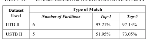
computation time. A single partition to split the image into two images was then iteratively tested across all possible splitting points. The splitting point that produced the most accurate matches was then chosen. The process was then repeated to create additional partitions until creating another partition no longer resulted in an improved matching accuracy. Although this greedy approach is not guaranteed to find the global optimum for partition size, it produces sufficient results while simultaneously reducing computation time. The results for this experiment are shown in Table VI, with those that exceeded or matched the results from experiment two in bold.

TABLE VI. DYNAMIC BINNING FOR THE IITD II AND USTB II DATASETS Dataset

Used

Type of Match

Number of Partitions Top-1 Top-5

IITD II 6 93.21% 97.13%

USTB II 5 51.95% 73.05%

previous experiment was achieved using only five partitions. Of particular interest is that the partitions in the upper range of the intensities seem to be smaller. The USTB II dataset was partitioned into five partitions, also differing from its fixed partition results. Results for this experiment show that dynamic binning produced slightly more accurate results on the IITD II dataset. However, this technique did not result in an overall higher accuracy on the USTB II dataset. Interestingly, however, it should be noted that the accuracy for dynamic partitioning was higher than its fixed partition counterpart when only considering the same number of partitions used. This demonstrates the potential of the dynamic partitioning approach and suggests that a true global optimum for partition size and number of partitions exists.

V. CONCLUSION

In this research, a PCA based algorithm called two dimensional multi-band PCA (2D-MBPCA) was presented and demonstrated on ear images. Each input image is partitioned into several images based on the intensity of its pixels, with each resulting image set being passed to PCA. Partitions of both fixed sizes and variable sizes were examined. Results show that this novel multi-band approach greatly outperforms a direct image comparison using PCA. Furthermore, variable sized partitions outperformed fixed sized on one of the two benchmark datasets. Despite the slightly reduced performance on the USTB II dataset, dynamic partitioning still showed merit when compared with an equivalent number of partitions for both datasets. This indicates that there is still potential for the dynamic partitioning approach, and that there is a potential global maximum for the image splitting problem. In future work, other optimization algorithms can be investigated to perform the dynamic partitioning. Furthermore, this splitting approach is not limited to the use of PCA with Euclidean distance. Another line of inquiry can investigate the use of binning with other feature extraction and ear matching algorithms.

ACKNOWLEDGMENT

This research has been funded under a knowledge transfer partnership by Innovate UK.

REFERENCES

[1] H. Nejati, L. Zhang, T. Sim, E. Martinez-Marroquin, and G. Dong, “Wonder ears: Identification of identical twins from ear images,” in Proceedings of the 21st International Conference on Pattern Recognition (ICPR2012), 2012, pp. 1201–1204.

[2] B. Victor, K. Bowyer, and S. Sarkar, “An evaluation of face and ear biometrics,” in Object recognition supported by user interaction for service robots, 2002, vol. 1, pp. 429–432 vol.1.

[3] K. Chang, K. W. Bowyer, S. Sarkar, and B. Victor, “Comparison and combination of ear and face images in appearance-based biometrics,” IEEE Transactions on Pattern Analysis and Machine Intelligence, vol. 25, no. 9, pp. 1160–1165, Sep. 2003.

[4] D. Querencias-Uceta, B. Ríos-Sánchez, and C. Sánchez-Ávila, “Principal component analysis for ear-based biometric verification,” in 2017 International Carnahan Conference on Security Technology (ICCST), 2017, pp. 1–6.

[5] Ž. Emeršič, V. Štruc, and P. Peer, “Ear recognition: More than a survey,” Neurocomputing, vol. 255, pp. 26–39, Sep. 2017.

[6] A. Pflug and C. Busch, “Ear biometrics: a survey of detection, feature extraction and recognition methods,” IET Biometrics, vol. 1, no. 2, pp. 114–129, Jun. 2012.

[7] M. A. Turk and A. P. Pentland, “Face recognition using eigenfaces,” in 1991 IEEE Computer Society Conference on Computer Vision and Pattern Recognition Proceedings, 1991, pp. 586–591.

[8] M. S. Nosrati, K. Faez, and F. Faradji, “Using 2D wavelet and principal component analysis for personal identification based On 2D ear structure,” in 2007 International Conference on Intelligent and Advanced Systems, 2007, pp. 616–620.

[9] J. C. Harsanyi and C. I. Chang, “Hyperspectral image classification and dimensionality reduction: an orthogonal subspace projection approach,” IEEE Transactions on Geoscience and Remote Sensing, vol. 32, no. 4, pp. 779–785, Jul. 1994.

[10] X. Jia and J. A. Richards, “Segmented principal components transformation for efficient hyperspectral remote-sensing image display and classification,” IEEE Transactions on Geoscience and Remote Sensing, vol. 37, no. 1, pp. 538–542, Jan. 1999.

[11] J. Zabalza et al., “Novel Folded-PCA for improved feature extraction and data reduction with hyperspectral imaging and SAR in remote sensing,” ISPRS Journal of Photogrammetry and Remote Sensing, vol. 93, pp. 112–122, Jul. 2014.

[12] “IIT Delhi Ear Database.” [Online]. Available: http://www4.comp.polyu.edu.hk/~csajaykr/IITD/Database_Ear.htm. [Accessed: 13-Mar-2018].