What Can I Get For It? A Theoretical and Empirical Re-Analysis
of the Endowment Effect
Pete Lunn
*and Mary Lunn
†Abstract:
We hypothesise and confirm a previously unnoticed pattern within
pre-existing data on the endowment effect, collected via seven experiments employing
the original design. Subjects with low valuations in binary choice relative to other
subjects set a proportionally higher willingness to accept. Those with high valuations
set a proportionally lower willingness to pay. The results challenge current theories,
including models of reference dependent preferences. The findings imply that
buyers and sellers consider not only their own preferences, but also their
perceptions of potential deals. We propose a model of optimal exchange that
rationalises this behaviour and accounts for the new findings.
JEL Codes: D03, D81
Keywords
: Endowment effect, willingness to pay, willingness to accept, loss aversion
* Corresponding Author, [email protected]
† Department of Statistics, University of Oxford, UK.
Acknowledgements :- This work is supported by a Research Development Initiative Grant to the first author from the Irish Research Council for the Humanities and Social Sciences (IRCHSS). We would like to extend special thanks to the authors of the two studies that granted us access to their data; especially to Nathan Novemsky and Robert Sugden for their generosity and assistance in this matter, and to the latter for incisive comments on an initial draft. We also thank Denis Conniffe, Liam Delaney, David Duffy, Andreas Glöckner, Daniel Goldstein, David Laibson, Laura Malaguzzi Valeri, attendees at the Royal Economic Society Annual Conference 2010, and those at the International Confederation for the Advancement of Behavioral Economics and Economic Psychology (ICABEEP) Conference 2010, for helpful comments relating to this work.
ESRI working papers represent un-refereed work-in-progress by researchers who are solely responsible for the content and any views expressed therein. Any comments on these papers will be welcome and should be sent to the author(s) by email. Papers may be downloaded for personal use only.
2
What Can I Get For It? A Theoretical and Empirical Re-Analysis
of the Endowment Effect
1. Introduction
More than two decades of research has thus far failed to settle the controversy over what lies behind the endowment effect. There remains no agreed explanation for the finding that experimental subjects endowed with an ordinary consumer good set the minimum price for selling the good about two (and sometimes more) times higher than the maximum price those without the good are prepared to pay for it.1 This large disparity between willingness-to-accept (WTA) and willingness-to-pay (WTP) has been replicated many times and is widely regarded as an example of irrational economic behaviour, because it implies that subjects deny themselves apparently beneficial exchanges. Failure thus far to identify decisively the cause of the endowment effect is problematic, because it suggests gaps in our understanding of simple exchanges, which are economically fundamental. The endowment effect has also been influential in the development of alternative theories of preferences and consumer choice.
This paper establishes that data produced by the original experimental design of Kahneman et al. (1990) contain a regularity that is inconsistent with most current theories of the endowment effect.2 Re-analysing data from two published studies, involving seven experiments conducted by leading researchers in the field,3 we explore whether WTA and WTP are systematically related to how individual subjects value the item to be traded relative to the valuations of other subjects. Our findings reveal that subjects in endowment
1
Our focus is the experimental design originated by Kahneman, Knetsch and Thaler (1990), in which subjects exchange goods and money. The endowment effect can also be demonstrated for non-monetary exchange of different goods (Knetsch, 1989). While the analysis we present can, in principle, be applied to both settings, the focus here is on the former design, because of the additional possibilities for quantitative analysis offered by monetary exchanges.
2 Throughout this paper we treat the term “endowment effect” as an empirical phenomenon. Our use
of the term does not imply any particular theoretical standpoint as to what causes the effect (cf. Plott and Zeiler, 2005).
3 The raw data were obtained following written requests to the corresponding authors of four studies
3
effect experiments are influences not only by their own preferences, but also by their perceptions of the preferences of others or, at least, prices others are prepared to pay or accept. The implication is that the present theoretical debate, which centres on whether the endowment effect is best explained by neoclassical or reference dependent preferences, effectively excludes one of the causes of the effect, possibly its primary cause. We offer an alternative theory that rationalises the observed behaviour, is consistent with the newly revealed empirical pattern, and may offer insight into related findings.
Section 2 summarises the theoretical debate surrounding the endowment effect and motivates our exploration of the potential role played by perceived preferences. Section 3 formalises the theory and derives two novel empirical hypotheses. Section 4 shows that current models, based on individual preferences over goods and money, either make no prediction or predict the opposite relationships to those hypothesised. Section 5 tests the hypotheses. Section 6 discusses the significance of the findings.
2. Theoretical Background
Following the original demonstrations of the endowment effect (Knetsch, 1989; Kahneman et al., 1990), one prominent theoretical perspective has held that individual preferences are reference dependent, meaning that they are systematically modified according to a reference state, initially identified with the individual’s current endowment (Tversky and Kahenman, 1991). Losses relative to the reference state are weighted more heavily than equivalent gains, i.e. individuals are loss averse. Reference dependent theories therefore abandon the independence axiom, which is central to the neoclassical assumption of stable preferences.
4
To account for such variation in the endowment effect, reference dependent models require additional degrees of freedom. Two alternatives have been proposed. Köszegi and Rabin (2006) contend that the reference state is defined by expectations and hence that variation in the strength of the endowment effect is due to variation in the expectation of making trades. Thus, if a change to experimental procedures or greater trading experience increases the expectation of trade, then losses and gains are evaluated relative to that expectation and the effect is reduced. Loomes, Orr and Sugden (2009) suggest instead that the strength of the endowment effect is determined by uncertainty about future preferences. When individuals decide on willingness to trade, they may be uncertain about realised utility at the time of final consumption. Some future “taste states” may entail prospective losses and thus carry greater weight in the decision, producing an endowment effect that is positively related to taste uncertainty and hence likely to attenuate with experience or experimental manipulations that reduce uncertainty.
These competing accounts of the endowment effect centre on the shape of the decision-maker’s preferences over goods and money. The present investigation considers an alternative, namely that when buyers and sellers set prices, they consider not only their own preferences but also the valuations of potential trading partners. From a theoretical perspective, incorporating perceptions of other agent’s valuations for exchange decisions is consistent with standard assumptions of models of consumer search and heterogeneous price-setting – a parallel on which we expand below. Our attention was also drawn to this possibility by some extant empirical work. Commonly, endowment effect experiments employ some form of the BDM value elicitation procedure (Becker, Degroot and Marschak 1964), requiring subjects to make a series of pair-wise choices for a range of prices, after which trades are executed at a single price selected at random, or a clearing price calculated by the experimenters. However, when Franciosi et al. (1996) instead conducted trading via a double-price auction, they recorded a smaller endowment effect. Similarly, Shogren et al. (1994) found that the WTA-WTP disparity reduced and disappeared across a series of rounds of second-price auctions. Double auctions and repeated second-price auctions provide feedback regarding the prices that others are prepared to accept and/or pay. Lastly, Van Boven, Dunning and Loewenstein (2000) provide direct evidence that subjects with lower WTP (WTA) estimate lower mean WTA (WTP) among potential trading partners.4
We develop and test a specific theoretical rationale for why subjects might set WTA or WTP not only with regard to their own valuation, but also with regard to their perceptions of the distribution of valuations across potential trading partners. Our approach begins with the
4 Our interpretation of this result differs from that of the authors, who argued that subjects were
5
observation that prices in most real markets are dispersed. Reviewing several decades of empirical results, Baye, Morgan and Scholten (2006) conclude that price dispersion is ubiquitous, even in modern competitive consumer product markets with an apparently low cost of price comparison. The decision faced by traders is, generally, whether to trade immediately or to hold out for a better deal. Optimal decision-making requires a trader to form and to consider a perception of the distribution of potential deals, rather than to compare the utilities of an item and a single price. Thus, perceptions of the preferences of potential trading partners can assist good decision-making in real markets. An optimising seller must ask “what can I get for it?”; an optimising buyer “what can I get one for?”.5
Consequently, we explore the possibility that subjects in endowment effect experiments extend a useful strategy, one which they habitually employ when trading in real markets, into a laboratory setting where it backfires. We propose that subjects are inclined to behave as if at the beginning of a sequence of trading opportunities. They aim to avoid deals with low margins above their own valuation because better ones ought to be possible, thus raising WTA and reducing WTP. Given that the standard endowment effect experiment is a one-shot game, where a single price determines which trades are executed, this represents a poor strategy and initially appears irrational. Yet it may reflect a habitual behaviour that has successfully adapted to sequential trading opportunities and price dispersion in real markets.
Previous empirical studies generally confine statistical analyses to comparisons between the mean and/or median values of WTA, WTP and frequently also the “choice equivalent” (CE), which is the amount of money required to be indifferent in a binary choice between gaining the item and gaining the money. Yet our theory implies that, to the extent that subjects can place their own valuation of the item within the population distribution of valuations, the relationships between WTA, WTP and CE should vary systematically across that distribution. This empirical conjecture is an attractive one to explore for two reasons. First, it can be tested with existing data, allowing inferences to be drawn rapidly across a number of previously peer-reviewed studies and experiments, with different conditions, subjects and experimenters. Second, as we will show, the hypotheses we develop regarding the pattern of variation contrast with the predictions of pre-existing theories. We now formalise the theory and hypotheses.
5 We choose here to emphasise buyers’ and sellers’ perceptions of the preferences of other market
6
3. Theory and predictions
3.1 Optimal Exchange with Sequential Opportunity
We have developed a relatively simple and highly generalised model of exchange that applies to both buyers and sellers. The complete model, with extensions and proofs, can be found in Lunn and Lunn (2009); here we present only what is essential to derive predictions. The model assumes optimising agents facing sequential opportunities to trade which come at a cost. The applicability of the model to the endowment effect depends on subjects in one-shot, one-price laboratory markets setting WTA and WTP as if they were in the more common real-world situation of facing sequential trading opportunities in a market with price dispersion. That is, they extend a strategy adapted for real markets to an artificial market where it is suboptimal.
Consider a seller who owns a good with a private value, x, and perceives the distribution of likely bids from potential buyers, Y, with mean μy and variance ςy2. The seller sets WTA as if
they expect to encounter bids in sequence {Y1, Y2, …, Yj, …}. Each bid entails a (small) cost, c,
which we call the “encounter cost”.6 The seller sets WTA = x + α, where α > 0 (as the seller will not sell at a loss), such that α corresponds to the minimum acceptable margin over and above the seller’s own valuation. Thus, the seller chooses α to maximise expected surplus:
This optimisation set-up shares features with some models of consumer search (most notably Reinganum, 1979), but is more general, most obviously in its application to sellers. It centres on a trade-off between holding out for a better ultimate price and incurring incremental costs. Provided the encounter cost is below an upper bound, the solution can be derived for any continuous distribution (Lunn and Lunn, 2009) such that α* satisfies
where F(y) is the cumulative distribution function of Y. In Equation 2, α* is decreasing in x and c. It can be further shown that where Y is unimodal and continuous, with a steadily
6
This cost can be conceived of as a search cost, but we do not describe it as such for reasons of generality. Active search is not necessary, while the cost could also reflect delay to final consumption or the cognitive load associated with considering more offers.
𝐸 𝑆 = 𝐸 𝑌 𝑌 > 𝑥 + 𝛼 − 𝑥 −
𝑐
Pr 𝑌 > 𝑥 + 𝛼
1 .
c = 1-F y dy
∞x+α*
7
decreasing probability of receiving bids higher than μy, α* is increasing in ςy (Lunn and Lunn,
2009).7
A symmetric set-up can be applied to the buyer, who sets WTP = x – β, where β > 0. For a perceived distribution of offers Z, with mean μz and variance ςz2, the buyer’s optimisation
problem is to set β to maximize
which (subject to an upper bound on c) yields the solution
where F(z) is the cumulative distribution function of Z. This time, β* is increasing in x, decreasing in c, and (under symmetrical assumptions about Z to those just described for Y above) increasing in ςz.
3.2 Predictions of the Optimal Exchange Model
The optimal exchange model straightforwardly predicts a WTA-WTP disparity, as WTA/WTP = (x + α)/(x – β). But it can also be used to make predictions regarding variation across individuals with different valuations, xi. Consider two sellers with valuations x1 and x2. If the
individuals are otherwise identical, such that they perceive the same distributions of bids and offers and face an identical encounter cost, then x1 + α1* = x2 + α2* and x1 – β1* = x2 –
β2*. Hence WTA/WTP is the same for both agents. However, if x1 < x2, then α1* > α2* and β1*
< β2* and, more importantly for present purposes
7
Agents in real markets may also be inclined to set a conservative initial value for WTA and WTP because they expect to update and improve their perception of the distribution of bids as they encounter others in the market, resulting in a better final deal. This again represents a poor strategy in the one-shot experimental market, but may nevertheless influence experimental results. A similar argument in relation to the endowment effect is made by Zhao and Kling (2004), who propose that an initially high WTA and low WTP might reflect the subject’s desire to learn more about their
preferences for the good before committing to a deal. Our alternative would be that the agent wishes to acquire more information about the preferences of other market participants. We do not
incorporate a mechanism for updating Y into the model here, however, as it would not change the contrasting predictions of our model relative to existing theories, which is our primary focus.
𝐸 𝑆 = 𝑥 − 𝐸 𝑍 𝑍 < 𝑥 − 𝛽 − 𝑐
Pr(𝑍 < 𝑥 − 𝛽) 3 ,
𝑐 = 𝐹 𝑧 𝑑𝑧 4 ,
𝑥−𝛽∗8 and
These expressions have analogues in empirical work and form the basis of our predictions. According to the model, x represents the individual’s private valuation of the good, such that in a binary choice the individual prefers the good to any amount less than x and prefers any amount more than x to the good. That is, x represents the “choice equivalent” (CE), a valuation obtained empirically alongside WTA and/or WTP in many studies, originating with Kahneman et al. (1990).8 Consequently, Equation 5 represents a counterintuitive claim. As measured by the ratio of WTA to CE, one of its standard measures, the endowment effect should be stronger for subjects who value the good least, all else equal. That is, for subjects with equivalent perceptions of potential deals, WTA/CE should be decreasing in CE. Similarly, according to Equation 6, CE/WTP should be increasing in CE. Again, this is initially counterintuitive, because it implies that individuals who value the good most should be willing to pay a smaller proportion of their valuation.
As stated, for given Y (Z) and c, all agents produce the same WTA (WTP), irrespective of xi. In
practice, there will be substantial variation across individuals in Y(Z) and c, driving substantial variation in WTA (WTP).9 Assuming no individual-level correlation between x and Y(Z) or c, the predictions implied by Equations 5 and 6 hold, all else equal. However, psychological findings such as “false consensus bias” (Ross, Greene and House, 1977) or “egocentric empathy gaps” (see Van Boven et al. 2000) suggest that Y(Z) may be biased in the direction of xi, i.e. those with low valuations may be inclined to assume lower willingness
to pay (accept) among others.10 Such correlations will tend to weaken the predicted relationships and it is hence important to establish the implications for our model and predictions. As a robustness check, we therefore conducted model simulations, using Equations 2 and 4 to solve for WTA and WTP, for empirically realistic valuation distributions, a range of encounter costs, and variable correlations between x and Y(Z). Appendix A presents details of the simulations plus illustrative output. Where perceptions of bids and offers are biased in the direction of own valuations, but otherwise approximate actual distributions of WTP and WTA, the model results in a WTA-WTP disparity, with WTA/CE declining and CE/WTP increasing in CE, as predicted. It requires high encounter costs
8 An alternative expression for this valuation, “equivalent gain”, is also sometimes used. 9 This is likely to be the case even where subjects are aware of a retail price for the item being
considered, for example if they are informed of the price of a college branded mug in the university shop. Such information represents only one common signal as to what others may be prepared to pay (accept). Empirically, Kahneman et al. (1990) show that in such circumstances there remains large variation in WTA and WTP, with a large WTA-WTP disparity. Given this result, variation in subjects’ perceptions of what others will pay and accept are also likely to remain.
10 We see less reason to suppose any general individual-level correlation between x and c, although it
is possible to envisage or design specific circumstances where one might exist.
(𝑥1+ 𝛼1∗) 𝑥1> (𝑥2+ 𝛼2∗) 𝑥2 (5)
9
combined with an extremely strong perceptual bias to nullify the predicted relationships. We therefore conclude that our predictions are robust to the possibility of perceptions being correlated with private valuations.
In practice, relative to the overall variation in perceptions (Y, Z), biases in the direction of xi
may well be small, because own valuations are just one of many potential influences regarding how others value an item. If so, then a further implication of the model is that CE will be only weakly correlated with WTA and WTP. This offers a possible explanation for differing empirical results regarding the level of CE relative to WTA and WTP. In some experiments average CE is not significantly different from average WTP (Novemsky and Kahneman, 2005), in others it lies between WTP and WTA but closer to the former (Kahneman et al., 1990; Franciosi et al., 1996), while in at least one experiment average CE is closer to average WTA (Bateman et al., 2005); contrasting findings that are mirrored by contrasting views among respective researchers about the existence or otherwise of loss aversion for money. Yet, according to the optimal exchange model, a high average CE relative to WTA and WTP would occur if the subject group as a whole tended towards underestimation of others’ valuations relative to their own, while low relative CE would occur if the group tended towards overestimation. Across experiments differing by type of item, familiarity of the item, and the availability of public signals about its value to others, such variability is likely and may therefore explain variation in the magnitude of average CE relative to WTA and WTP.
3.3 Empirical Hypotheses
In a standard endowment effect experiment, different valuations are obtained from different subjects, so it is not possible to obtain within-subject comparisons of CE, WTA and WTP. Nevertheless, a between-subjects comparison of the distributions suffices to test the predictions. The model implies that individuals with lower CE will, all else equal, have a higher WTA/CE and lower CE/WTP. If the distributions are matched by quantile, therefore, WTA/CE should be greater for lower quantiles. In fact, this test is conservative. To the extent that changing the valuation from CE to WTA or WTP is not order preserving, both predicted relationships are likely to be underestimated by a between-subjects comparison relative to a within-subjects comparison. Thus, our empirical hypotheses are as follows:
10
Hypothesis 2: When the distributions of willingness-to-pay (WTP) and choice equivalent (CE) valuations are matched by quantile, CE/WTP will increase for higher quantiles.
In practice, separate analysis by quantile is hampered by the small sample sizes of endowment effect experiments. We therefore test the hypotheses in two ways. First, we simply divide paired sets of WTA-CE (CE-WTP) observations into two quantiles either side of the median, then compare mean WTA/CE (CE/WTP) separately for the bottom quantile (Q1) and the top quantile (Q2). Second, we pool data across experiments by matching up realisations of order statistics, which allows us to place valuations on a common scale and thus to produce a more fine-grained analysis of the variation in the two ratios by quantile.
4. Predictions of Existing Models
Before presenting empirics, this section aims carefully to derive equivalent empirical predictions from the reference dependent and neoclassical models briefly reviewed in Section 2.
4.1 Prediction of Tversky and Kahneman (1991)
In Tversky and Kahneman (1991), the extent of the endowment effect is straightforwardly determined by the extent of loss aversion implied by the shape of the value function according to Prospect Theory (Kahneman and Tversky, 1979). Since there is no reason to believe that the shape of this value function is systematically related to the location of an individual subject’s CE within the population distribution of CEs for a given item, the model predicts no variation in either WTA/CE or CE/WTP with CE. Tversky and Kahneman (see also Novemsky and Kahneman, 2005) further argued that loss aversion does not apply to goods intended for resale rather than final consumption, including money. Thus, according to this version of the theory, it is also the case that CE/WTP = 1.
4.2 Prediction of Köszegi and Rabin (2006)
11
accurately assess their valuation relative to the valuations of others, expectations of trade ought indeed to be influenced. Subjects with a relatively low CE should be most likely to expect to sell, because they perceive that others tend to value the good more highly. Those with relatively high CE should, conversely, be least likely to expect to sell. Consequently, WTA/CE should be increasing in CE. In contrast, buyers with a relatively low CE should least expect to buy and thus CE/WTP should be decreasing in CE. In other words, the model predicts the opposite of Hypotheses 1 and 2.
4.3 Prediction of Loomes et al. (2009)
Loomes et al. propose that the endowment effect results from uncertainty regarding utility at the time of final consumption, which may vary according to the agent’s “taste state”, e.g. variable mood and hunger may determine final utility from a chocolate bar. Formally, Loomes et al. incorporate this uncertainty by specifying the subjective value of moving from reference bundle z to an alternative consumption bundle x as
where π(sh) is the subjective probability of taste state sh, which entails the utility function
uh(.) over x and z, but where φ(.) is concave, such that utility losses are ultimately weighted
more heavily than gains of equivalent size. Consequently, an endowment effect results when sufficient taste states exist in which uh(x) – uh(z) < 0, leading v(x, z) to be potentially negative
even where bundle x has higher expected utility than bundle z.
In Appendix B, we use this formulation to derive an expression for CE and to show that for a given set of possible taste states WTA/CE is increasing in CE – the opposite of Hypothesis 1. Intuitively, given two agents endowed with the item who possesses the same taste states, the agent with the higher marginal utility for the item (higher CE) has a greater or equal probability of final utility loss following exchange and hence sets a greater or equal WTA/CE. By similarity, the equivalent opposite prediction to Hypothesis 2 arises for CE/WTP. The model could be augmented by positing a systematic relationship between the marginal utilities of goods and the range of possible taste states, which might avoid variation in WTA/CE and CE/WTP with CE, but it is difficult to see how it could generate Hypotheses 1 and 2.
4.4 Predictions of non-reference dependent theories
Plott and Zeiler (2005) do not offer a formal model of the endowment effect, but instead put it down to subject “misconceptions” regarding the experimental set-up, arguing that
12
neoclassical theory applies once such misconceptions are cleared up. Since there is no reason to assume that misconceptions are more or less likely among subjects with high valuations of the item than among those with low valuations, this account does not predict variation in WTA/CE and CE/WTP with CE.11
Lastly, one recent model (Kling, List and Zhao 2010; see also Zhao and Kling 2004) shares with our own the idea that despite the BDM mechanism, subjects treat the experimental situation as dynamic, rather than as a one-shot game with pay-offs consisting of money or final consumption of the good. Kling et al.’s model can be summarised as
valuation + Obuying = E(value of item) + Oselling
where the valuation is either WTP or WTA and Obuying and Oselling are the option values of
trying to buy the item later and trying to sell the item later respectively. The model produces a WTA-WTP disparity if buyers and sellers possess asymmetric perceptions of option values. Specifically, Kling et al. hypothesise that lack of selling experience among buyers means that the option value of selling is low, while cognitive dissonance increases it for those cast in the role of sellers. Experienced traders conform to the more straightforward neoclassical prediction of no endowment effect.
Given this account, subjects asked for their CE ought to have the same option values as buyers, since they have the same experience and no exposure to cognitive dissonance by being designated as sellers. This model therefore predicts WTP = CE. With respect to WTA/CE, it is difficult to formulate a prediction without making additional assumptions about whether and how the two option values scale with the expected value of the item. 12 If it were hypothesised that option values do not scale with expected value, such that they are proportionally smaller for individuals with higher expected values, WTA/CE could decrease with CE, in line with Hypothesis 1.13
11 The argument can be made that employing a strategy based on our optimal exchange model when
facing the BDM value elicitation mechanism (or similar) amounts to a “misconception”. But how one best interprets this behaviour and its implications for neoclassical consumer theory is not
straightforward. We return to the issue in the final section. 12
There is some ambiguity in Kling et al. (2010) with respect to option values, which are identified at different points with transaction costs, “difficulty” of buying/selling, and additional time to reduce the uncertainty surrounding perceptions of value and market price. Depending which of these definitions is adopted, an argument can be made either way regarding whether option values scale with
expected value.
13 Chambers and Melkonyan (2009) also offer a formal model that maintains standard neoclassical
13
5. Empirics
Having derived contrasting predictions from our optimal exchange theory and from current theories of the endowment effect, we concluded that the most robust way to test our hypotheses was to re-analyse pre-existing data. As well as avoiding needless experimental replication, this approach has the added advantages of permitting the hypotheses to be tested across a large number of experiments, which were carried out with a range of items, different subject pools in different countries, and different experimenters, who were unaware at the time of the hypotheses at issue.
5.1 Data
We employ raw valuation data from six experiments conducted by Novemsky and Kahneman (2005) and one undertaken by Bateman et al. (2005). The scope of these studies allows us to test our hypotheses with nine paired sets of WTA-CE valuations and five paired sets of CE-WTP valuations, all obtained using the basic experimental design of Kahneman et al. (1990) , with only minor modifications.14 Both WTA-CE and CE-WTP comparisons involve at least three different consumer items and subjects located in three different countries (USA, Canada, UK). Each set of observations is derived from a different subject group, so all comparisons are between-subject. The five sets of CE valuations in the CE-WTP comparison also feature in the WTA-CE comparison.
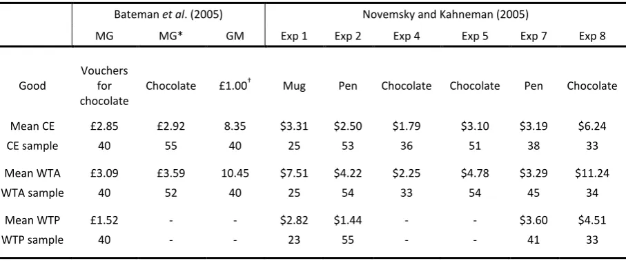
A summary of the data is provided in Table 1, together with mean valuations and sample sizes. The labelling of the experiments and treatments is preserved from the original studies. Before conducting additional analyses, we ensured that we could use the raw data to reproduce the published median and/or mean values from the two studies, which we could do for all 23 distributions of valuations without difficulty.
CE) and the sharpness of the corner-point (which determines relative WTA and WTP). In the absence of any rationale for such a relationship, it is not possible to make precise predictions.
14 Minor differences include the exact wording of instructions, whether subjects were confronted with
14 Table 1: Summary of data
Bateman et al. (2005) Novemsky and Kahneman (2005)
MG MG* GM Exp 1 Exp 2 Exp 4 Exp 5 Exp 7 Exp 8
Good
Vouchers for chocolate
Chocolate £1.00† Mug Pen Chocolate Chocolate Pen Chocolate Mean CE £2.85 £2.92 8.35 $3.31 $2.50 $1.79 $3.10 $3.19 $6.24
CE sample 40 55 40 25 53 36 51 38 33
Mean WTA £3.09 £3.59 10.45 $7.51 $4.22 $2.25 $4.78 $3.29 $11.24
WTA sample 40 52 40 25 54 33 54 45 34
Mean WTP £1.52 - - $2.82 $1.44 - - $3.60 $4.51
WTP sample 40 - - 23 55 - - 41 33
†
In this case, subjects in the WTA condition were endowed with one pound sterling and various prices bid in numbers of chocolates, while subjects in the CE condition chose between a gain of one pound or varying numbers of chocolates. The unit of currency here is therefore the chocolate.
5.2 Statistical Methods
There is divergence within the literature regarding whether to compare median or mean valuations. With respect to the median, its reliability as a summary statistic is affected by the tendency for valuations to be drawn towards salient prices (e.g. $5.00).15 With respect to the mean, bias results from the small number of subjects whose valuations lie above the maximum price, i.e. those who even at the highest price still buy (WTP condition), refuse to sell (WTA), or choose the item rather than the money (CE). This cap on valuations potentially reduces the mean by an unknown amount, with the impact likely to be greater for WTA. In the data, while just 38 of the total of 940 subjects had valuations above the maximum price, at least one subject did so in 15 of the 23 sets of observations, including all nine WTA sets.
Considering these issues, and given that the primary aim is to make separate comparisons for upper and lower quantiles, which requires disaggregation of already small samples, the priority is to minimise measurement error and to maximise the use of available variation in the data. This results in a preference for a comparison of means, requiring us to nullify the problem of maximum valuations. Our solution is, for each pair-wise comparison, to discard observations at the maximum and also to discard the matching top percentiles of the comparison observations. We then define the lower quantile, Q1, to be those observations below the median of the remaining truncated distribution of valuations, and the higher quantile, Q2, to be those observations above the median.
15
15
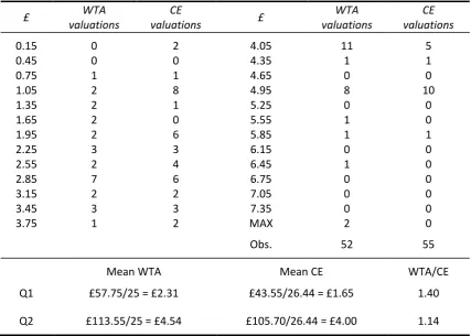
[image:15.595.84.512.364.669.2]To illustrate and to provide a feel for the data, Table 2 shows the detailed calculation for the MG* comparison of WTA and CE from Bateman et al. (2005), which involved subjects stating CE or WTA for a box of chocolates. The data are expressed as frequencies at valuations that correspond to the midpoints of intervals of £0.30, derived from a list of 26 prices with a minimum of £0.00 and a maximum of £7.50. Salient prices are evident as frequency spikes. For instance, the salience of the £5.00 price is revealed by the fact that eight of 52 WTA subjects were prepared to sell their chocolate at £5.10 but not at £4.80, while ten of 55 CE subjects preferred the chocolate over £4.80 but £5.10 over the chocolate. Two WTA subjects would not sell at the maximum price of £7.50. We exclude these observations and calculate the mean of the lowest 25 observations (Q1) and the highest remaining 25 observations (Q2), then compare these to the mean of the lowest 26.44 and highest 26.44 CE observations, which are the matching CE valuations. For Q1, WTA/CE is 1.40, while for Q2 it is 1.14.
Table 2: Raw frequency data and calculation of WTA/CE for Q1 and Q2 in comparison MG*, derived from Bateman et al. (2005)
£ WTA
valuations
CE
valuations £
WTA valuations
CE valuations
0.15 0 2 4.05 11 5
0.45 0 0 4.35 1 1
0.75 1 1 4.65 0 0
1.05 2 8 4.95 8 10
1.35 2 1 5.25 0 0
1.65 2 0 5.55 1 0
1.95 2 6 5.85 1 1
2.25 3 3 6.15 0 0
2.55 2 4 6.45 1 0
2.85 7 6 6.75 0 0
3.15 2 2 7.05 0 0
3.45 3 3 7.35 0 0
3.75 1 2 MAX 2 0
Obs. 52 55
Mean WTA Mean CE WTA/CE
Q1 £57.75/25 = £2.31 £43.55/26.44 = £1.65 1.40 Q2 £113.55/25 = £4.54 £105.70/26.44 = £4.00 1.14
16
and thus to pool observations across experiments. Straightforward standardisation via the mean and standard deviation is hampered by the observations at maximum valuations, which bias both estimates. We consequently adopt an alternative approach of matching up realisations of order statistics to calculate an observation-by-observation estimate of the relevant ratio.
The following describes the method for the WTA-CE comparison. The WTA and CE observations are separately ordered, then the order statistics are rescaled to fit the interval [0, 100]. The realisation of each order statistic in the smaller of the two samples is then matched up with its corresponding realisation(s) in the larger sample. In six of the nine paired sets, there is a small difference in sample size, with the result that most observations in the smaller sample do not have a precise match, but correspond to a position between two realisations of order statistics in the larger sample. We therefore match to a linear weighted average of these two adjacent realisations in the larger sample. This matching procedure produces an estimate of WTA/CE for each valuation in the smaller sample. We exclude valuations at zero and at the maximum. We also exclude valuations at the lowest available price, which is smaller than the price interval and hence makes the possible matches too coarse, introducing a high degree of noise. (For example, using the valuations in Table 2, the only possible matches for the price of £0.15 produce ratios of 1, 3, 5..., while for the £0.45 price the available ratios are 1, 1.66, 2.33...). We then pool the data, which produces 312 separate estimates of WTA/CE, with the extremities of the value distribution somewhat under-represented because of the discarded observations. The equivalent procedure for WTP produces 153 separate estimates of CE/WTP.
Given that the data are pooled across experiments, which are sufficiently different to produce considerable variation in the strength of the observed endowment effect (see Table 1), these ratios calculated by matching up realisations of order statistics are naturally subject to noise, especially at the lower end of the valuation distribution, where price intervals are proportionally more coarse. Nevertheless, as the following section shows, this more fine-grained method offers additional insight into how the two ratios vary across the valuation distribution, all else equal. It therefore complements the two-quantile approach.
5.3 Two-Quantile Results
17
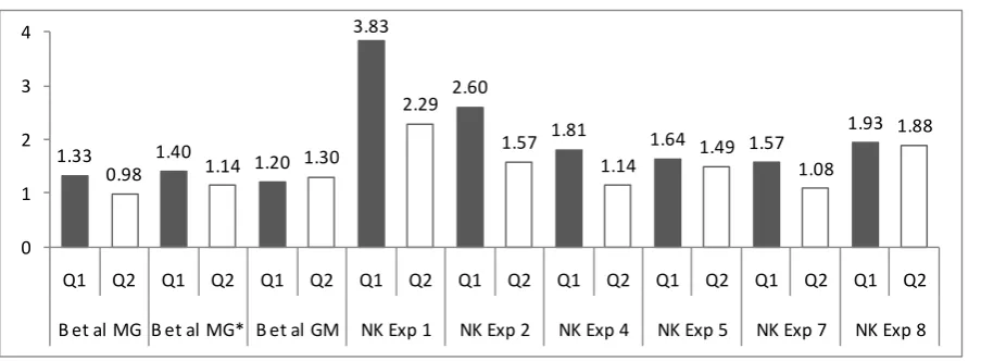
[image:17.595.76.528.182.348.2]subjects had to set their price for buying, selling or choosing £1.16 The likelihood of observing the data in Figure 1 if, in fact, the probability of observing greater WTA/CE for Q1 than Q2 were 0.5, is 10/512 (p=0.020). The data, therefore, support Hypothesis 1.
Figure 1: Comparison of WTA/CE for low and high quantiles. WTA/CE is greater for the lower quantile (Q1) in eight of nine paired sets of observations.
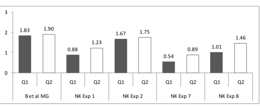
Figure 2 reveals the outcome of the CE-WTP comparison, for which the opposite pattern emerges, such that CE/WTP is greater in Q2 for all five comparisons. The chance of observing this pattern of results if, in fact, the probability of CE/WTP being greater for Q2 were 0.5, is 1/32 (p=0.031). These results support Hypothesis 2. Taken together, the two-quantile comparisons therefore provide support for both hypotheses.17 This two-quantile analysis is, however, very coarse, such that it could be driven by the behaviour of a relatively small subset of subjects.
16
In the original study, Bateman et al. report different implicit preferences when the “response mode” was chocolates instead of money, with subjects apparently valuing chocolate much less relative to money once valuations were requested in units of chocolate. This might or might not be related to our findings, but does suggest that the unusual nature of the task also had an unusual impact on the setting of CE and WTA.
17 The two p-values associated with Hypotheses 1 and 2 should not be regarded as independent,
because five sets of CE observations are common to both WTA-CE comparisons and CE-WTP comparisons. Note, however, that any statistical variation that increases mean CE for Q1 relative to Q2 and hence increases the probability that the data conform to Hypothesis 1, simultaneously decreases the probability that the data support Hypothesis 2
1.33 0.98
1.40
1.14 1.20 1.30 3.83
2.29 2.60
1.57 1.81
1.14 1.64 1.49 1.57 1.08
1.93 1.88
0 1 2 3 4
Q1 Q2 Q1 Q2 Q1 Q2 Q1 Q2 Q1 Q2 Q1 Q2 Q1 Q2 Q1 Q2 Q1 Q2
18
Figure 2: Comparison of CE/WTP for low and high quantiles. CE/WTP is greater for the higher quantile (Q2) in each of five paired sets of observations.
5.4 Pooled Results
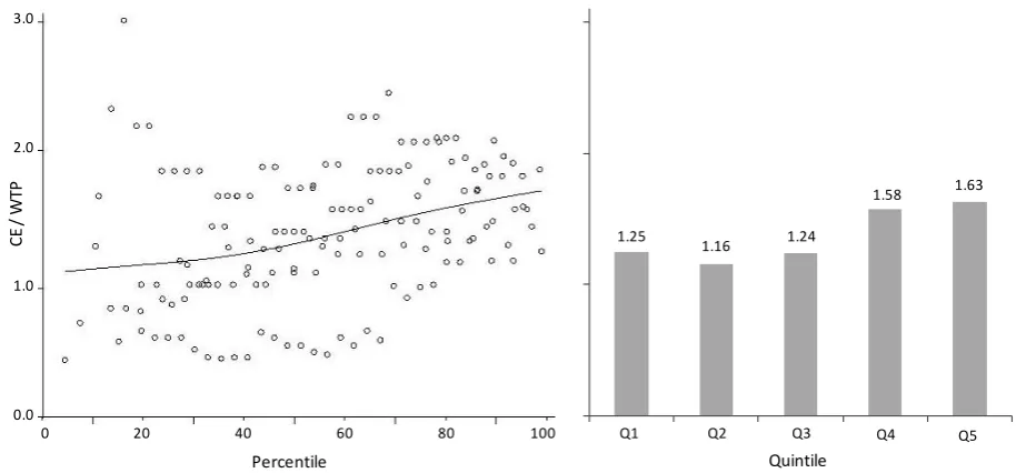
Figure 3 shows the variation in WTA/CE when the data are instead pooled across experiments by matching up realisations of order statistics. The panel on the left plots all valid estimates. The fitted curve employed to summarise the relationship is a cubic spline. The right panel shows mean WTA/CE by quintile. The decline in WTA/CE with CE occurs steadily across the valuation distribution, suggesting that the two-quantile results are not due to the behaviour of a small subset of individuals within the lower or higher quantile. Figure 4 provides the equivalent analysis for CE/WTP. Since a greater proportion of WTP valuations occur at low prices and the sample is smaller, the data are noisier. Nevertheless, the increase in CE/WTP with CE is again clear and suggests that the two-quantile results are not due to a subset of observations, but that Hypothesis 2 holds across the valuation distribution. This finer-grained analysis therefore provides additional support for Hypotheses 1 and 2.
1.83 1.90
0.88
1.23
1.67 1.75
0.54
0.89 1.01
1.46
0 1 2 3
Q1 Q2 Q1 Q2 Q1 Q2 Q1 Q2 Q1 Q2
19
Figure 3: Variation in WTA/CE across the valuation distribution with pooled data. Individual observations (left) and mean WTA/CE by quintile (right).
Figure 4: Variation in CE/WTP across the valuation distribution with pooled data. Individual observations (left) and mean CE/WTP by quintile (right).
5.5 Quantitative Implications for Loss Aversion
The results presented in the previous two sections run contrary to the predictions of reference dependent models, as derived in Sections 4.1-4.3. Yet could it still be argued that WTA-WTP disparities are due to loss aversion and that the relationships evident in Figures 1-4 above reflect some kind of separate, “second-order” phenomenon? In theory, any
1.97
1.71
1.57
1.37
1.25
Q1 Q2 Q3 Q4 Q5
Quantile Percentile
5.0
4.0
3.0
2.0
1.0
0 20 40 60 80 100
W
TA
/
CE
Percentile Quintile
3.0
2.0
1.0
0.0
0 20 40 60 80 100 Q1 Q2 Q3 Q4 Q5
1.25
1.16 1.24
1.58 1.63
CE
/
W
[image:19.595.75.537.412.625.2]20
additional factor that influences CE independently of WTA and WTP, or vice-versa, could produce systematic variation in WTA/CE and CE/WTP across the valuation distribution.
The scales of the effects reported above lead us to reject this interpretation, however. Figure 3 reveals that a seller in the bottom quintile of the valuation distribution requires a proportional margin [(WTA – CE )/CE] that is almost four times greater than a seller in the top quintile, while Figure 4 shows that a buyer in the top quintile requires two-to-three times as much proportional surplus [(CE – WTP)/CE] as a buyer in the lower two quintiles.18 A consequence of the scale of these two effects is that the position of CE relative to WTA and WTP, which has previously been considered an indication of the relative extents of loss aversion for goods and money respectively (Novemsky and Kaheman, 2005; Bateman et al. 2005), changes very considerably across quintiles. Based on the quintile means in Figure 3 and 4, the implied ratios in which CE divides the WTP-WTA interval are: 17:83 (Q1), 16:84 (Q2), 25:75 (Q3), 50:50 (Q4), 61:39 (Q5). Thus, if a factor additional to loss aversion drives our results then, firstly, it overrides loss aversion for goods and money when CE is compared with other valuations and, secondly, it is able to alter CE independently of WTA and WTP by the equivalent of at least 45% of the gap between WTA and WTP. This does not, therefore, look like a second-order phenomenon. Furthermore, given the various sources of noise in the data, including the between-subjects design, our results probably underestimate the true scale.
6. Discussion
The optimal exchange theory produces novel empirical predictions about the relationships between three valuations measured in the original experimental paradigm of Kahneman et al. (1990): willingness-to-accept (WTA), willingness to pay (WTP) and choice equivalent (CE). The subsequent empirical re-analysis, based on data gathered using that original paradigm, strongly supports the predictions. Sellers with low valuations set WTA proportionally higher with respect to CE than those with high valuations, while buyers with high valuations set WTP proportionally lower with respect to CE than those with low valuations.
The findings run contrary to predictions derived from existing models. With respect to reference dependent models, in order to be consistent with the empirical pattern revealed in Section 5, loss aversion would have to be greater for those who value a good least relative to other market participants. Meanwhile, loss aversion for money would have, firstly, to
18 We don’t read much into the difference in the scale of the two effects because, as the left panel of
21
exist (cf. Novemsky and Kahneman 2005) and, secondly, to be greater for those who value a good most. Alternatively, it would have to be argued that loss aversion is not the main determinant of the relativities between CE and WTP and WTA, and that some overriding factor strongly influences CE independently of WTA and WTP (or vice-versa). These propositions seem arbitrary and we hence favour a theory that can explain both WTA-WTP disparities and their relationship to CE within the same model.
Thus, while our results do not prove that loss aversion has no role, they do cast considerable doubt over whether it is the primary cause of the endowment effect, as reported by Kahneman et al. (1990). There is, of course, a separate body of evidence for loss aversion in other consumer decision-making contexts (see Rick, in press, for recent review).
In addition to predicting the novel empirical pattern above, the optimal exchange model is consistent with some other recent results relating to variation in WTP and/or WTA. Kling et al. (2010) provide direct evidence that WTA-WTP disparities are the result of dynamic considerations, showing that WTA and WTP valuations are related to the perceived difficulty of buying or selling the good in future and that they respond to explicit manipulations of the cost of delaying or reversing the trade. Mazar, Köszegi and Ariely (2010) supply experimental evidence that WTP responds to perceptions of the distribution of market prices during sequences of real exchanges. Lastly, meta-analyses reveal that WTA-WTP disparities are proportionally greater for goods that are hard to value (Horowitz and McConnell, 2002; Sayman and Öncülar, 2005). An extended formalisation of our model accounts for this by proposing that individuals use their own uncertainty over value as a signal regarding the degree of uncertainty in the valuations of others and, hence, the likely dispersion of bids and offers (Lunn and Lunn, 2009).
22
One possible interpretation of our theory is that it effectively amounts to a neoclassical account, since the model we offer assumes rational, optimising agents. This is not our own interpretation, however. Our optimal exchange model derives from a perspective in which the primary challenge facing traders is a dynamic decision context characterised by uncertainty in perceptions of value and prices. From this perspective, the significance of the endowment effect as an empirical phenomenon is not its implications for the validity of neoclassical preference axioms. Rather, the endowment effect questions the applicability of the standard, comparative-static, neoclassical preference model, because it shows that the model does not accurately predict behaviour in simple incentive compatible exchanges. For instance, Plott and Zeiler (2005) refer to the possibility that when a seller is asked for a price “...natural instincts might persuade him to announce an amount higher than his actual valuation” (p.538, emphasis added). They then design an experiment that aims to overcome such instincts in order to assess “true” preferences, involving extensive initial training of subjects in the BDM mechanism and instruction as to why stating the “true” valuation is the dominant strategy. Yet the resulting experimental design still does not entirely extinguish WTA-WTP disparities (Isoni et al. forthcoming). Instinctive behaviour in simple exchanges may depart from neo-classical predictions because it has adapted to cope with dynamic trading environments characterised by price dispersion and approximate perceptions of price and value. These are not central features of the neoclassical framework, which therefore struggles to account for empirical findings relating to simple exchanges, whether preference axioms hold or otherwise.
Finally, we are conscious that our optimal exchange theory, while producing novel and accurate predictions, offers just one potential mechanism via which buyers and sellers might be influenced by their perceptions of the preferences of others. There are other possibilities. For instance, an intriguing alternative for future research to consider is whether subjects in endowment effect experiments are averse to uneven splits of the transaction surplus and thus prepared to make sacrifices to avoid them. Put simply, rather than holding out for a good price, as we have hypothesised, perhaps subjects hold out for a fair price. Thus, sellers who perceive that most other people have a higher valuation than their own might set WTA proportionally higher, over and above their private value, to avoid a high probability of selling to someone who would gain the lion’s share of the total surplus generated. The obvious analogy here is to the Ultimatum Game (Güth, Schmittberger and Schwarze 1982) and to variation in willingness to pay for goods from suppliers with apparently different costs (Thaler 1985). With the present data, we cannot differentiate between this alternative theory and our optimal exchange theory; both imply Hypotheses 1 and 2.
23
References
Bateman, I., Kahneman, D., Munro, A., Starmer, C. And Sugden, R. (2005). Testing Competing Models of Loss Aversion: An Adversarial Collaboration. Journal of Public Economics, vol. 89, pp. 1561-80.
Baye, M.R., Morgan, J. and Scholten, P. (2006). ‘Information, Search and Price Dispersion’, in (Henderschott, T., ed.), Handbook on Economics and Information Systems, pp. 326-76, Amsterdam: Elsevier.
Becker, G.M., DeGroot, M.H. and Marschak, J. (1964). ‘Measuring utility by a single response sequential method’, Behavioural Science, vol. 9, pp. 226-32.
Chambers R.G. and Melkonyan T.A. (2009). Buy low, sell high: Price gaps and neoclassical theory. Journal of Mathematical Economics, vol. 45, pp. 720-9.
Franciosi, R., Kujal, P., Michelitsch, R., Smith, V. and Deng, G. (1996). ‘Experimental tests of the endowment effect’, Journal of Economic Behaviour and Organization, vol. 30, pp. 213-26.
Güth, W., Schmittberger, R. and Schwarze, B. (1982). An Experimental Analysis of Ultimatum Bargaining, Journal of Economic Behavior and Organization, vol. 3, pp. 367-88.
Horowitz, J.K. and McConnell, K.E. (2002). ‘A Review of WTA/WTP Studies’, Journal of Environmental Economics and Management, vol. 44, pp. 426-47.
Isoni, A., Loomes, G. and Sugden, R. (forthcoming). The Willingness to Pay-Willingness to Accept Gap, the "Endowment Effect", Subject Misconceptions, and Experimental Procedures for Eliciting Valuations: A Reassessment. American Economic Review.
Kahneman, D. and Tversky, A. (1979). Prospect Theory: An Analysis of Decision under Risk. Econometrica, vol. 47, pp. 263-291.
Kahneman, D., Knetsch, J.L. and Thaler, R.H. (1990). ‘Experimental Tests of the Endowment Effect and the Coase Theorem’, Journal of Political Economy, vol. 98, pp. 1325-48.
Kling, C.L., List, J.A. and Zhao, J. (2010). A Dynamic Explanation of the Willingness to Pay and Willingness to Accept Disparity. NBER Working Paper No. 16483.
Knetsch, J.L (1989). ‘The Endowment Effect and Evidence of Nonreversible Indifference Curves’, American Economic Review, vol. 79, pp. 1277-84.
Köszegi, B. and Rabin, M. (2006). ‘A model of reference-dependent preferences’, Quarterly Journal of Economics, vol. 121, pp. 1133-66.
List, J.A. (2003). ‘Does Market Experience Eliminate Market Anomalies?’, Quarterly Journal of Economics, vol. 118, pp. 41-71.
List, J.A. (2004). ‘Neoclassical Theory versus Prospect Theory: Evidence from the Marketplace’, Econometrica, vol. 72, pp. 615-25.
24
Lunn, P.D. and Lunn M. (2009). A Computational Theory of Exchange: Willingness to Pay, Willingness to Accept and the Endowment Effect. ESRI Working Paper 327.
Mazar, N., Köszegi, B. and Ariely, D. (2010). Price-Sensitive Preferences. Working Paper, University of Califormia.
Novemsky, N. and Kahneman, D. (2005). The Boundaries of Loss Aversion. Journal of Marketing Research, vol. 42, pp. 119-28.
Plott, C.R. and Zeiler, K. (2005). ‘The Willingness to Pay-Willingness to Accept Gap, the "Endowment Effect," Subject Misconceptions, and Experimental Procedures for Eliciting Valuations’, American Economic Review, vol. 95, pp. 530-45.
Plott, C.R. and Zeiler, K. (2007). ‘Exchange Asymmetries Incorrectly Interpreted as Evidence of Endowment Effect Theory and Prospect Theory?’, American Economic Review, vol. 97, pp. 1449-66.
Reinganum, J.F. (1979). ‘A Simple Model of Equilibrium Price Dispersion’, Journal of Political Economy, vol. 87, pp. 851-8.
Rick, S.I. (in press), “Losses, Gains, and Brains: Neuroeconomics Can Help to Answer Open Questions about Loss Aversion,” Journal of Consumer Psychology.
Ross, L., Green, D. and House, P. (1977). The "False Consensus Effect": An Egocentric Bias in Social Perception and Attribution Processes Journal of Experimental Social Psychology, vol. 13, pp. 279-301.
Sayman, S. and Öncülar, A. (2005). Effects of Study Design Characteristics on the WTAWTP Disparity: A Meta-analytical Framework. Journal of Economic Psychology, vol. 26, pp. 289-312.
Shogren, J.F., Shin, S.Y., Hayes, D.J. and Kliebenstein, J.B. (1994). ‘Resolving Differences in Willingness to Pay and Willingness to Accept’, American Economic Review, vol. 84, pp. 255-70.
Thaler, R. (1985). ‘Mental Accounting and Consumer Choice’, Marketing Science, vol. 4, pp. 199-214.
Tversky, A. and Kahneman, D. (1991). ‘Loss Aversion in Riskless Choice: A Reference-Dependent Model’, The Quarterly Journal of Economics, vol. 106, pp. 1039-61.
Van Boven, L., Dunning, D. and Loewenstein, G. (2000). Egocentric Empathy Gaps Between Owners and Buyers: Misperceptions of the Endowment Effect. Journal of Personality and Social Psychology, vol. 79, pp. 66-76.
25
Appendix A: Simulations to Assess the Impact of Correlation Between Private
Values and perceptions of Bids and Offers
Empirically, all three valuation distributions (WTP, CE, WTA) are approximately log-normal, once the tendency for valuations to be drawn to salient prices is discounted. We therefore assume that private values, xi, are distributed as log X ~ N(μ1, ς1) and that (in the case of
setting WTA) agents perceive bids distributed as log Y ~ N(μ2, ς2). Correlation between X and
Y is introduced by setting P1 = (X – μ1)/ς1 and P2 = (Y – μ2)/ς2, where P1 and P2 have a joint
bivariate normal distribution with corr(P1, P2) = ρ. We then use Equation 2 of the optimal
exchange model (see Section 3.1) to simulate the setting of WTA for a range of xi and any
combination of μ1, ς1, μ2, ς2, c and ρ. (The set-up for WTP is identical, with Y substituted by Z
and the solution supplied by Equation 4).
To explore the effects of individual-level correlation between private values and perceptions of bids (offers), we set μ1, ς1, μ2 and ς2 to match the parameters of the empirically observed
valuation distributions. Thus, the distribution of private values (X) is parameterised using the observed CE valuations. For sellers, the perceived distribution of bids (Y) is parameterised using observed WTP valuations, but with the distribution biased by own valuation as determined by ρ. Similarly, buyers perceive offers (Z) that match the observed WTA distribution with a bias dictated by ρ.
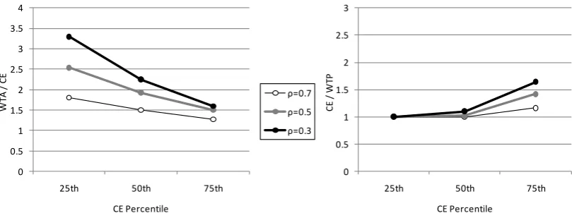
Given this set-up, we explore how WTA/CE and CE/WTP vary with CE for different values of c and ρ. Figure A1 displays typical output. The valuation distributions in this case are parameterised according to the observed valuations of NK Exp 8, which is in effect the median experiment with respect to the extent of disparity between valuations (see Section 5, Table 1). The item is a bag of Godiva chocolates with mean CE of $6.24. Figure A1 is based on an encounter cost, c, of $0.20. Results are given for agents with CE valuations at the 25th, 50th and 75th percentile and three values of ρ (0.3, 0.5, 0.7).
26
Figure A1: Example of simulated WTA/CE (left) and CE/WTP (right) against CE for
various degrees of correlation between private values,
x
i, and perceptions of bids
(
Y
) and offers (
Z
) respectively.
0 0.5 1 1.5 2 2.5 3
25th 50th 75th
C
E
/
W
TP
CE Percentile 0
0.5 1 1.5 2 2.5 3 3.5 4
25th 50th 75th
W
TA
/
C
E
CE Percentile
27
Appendix B: Prediction of Loomes et al. (2009)
From Loomes et al., bundle x is weakly preferred to bundle y at reference bundle z if
)
,
(
)
,
(
x
z
y
z
where ; final consumption occurs ina “taste state”, sh (h = 1, ..., m), with probability π(sh); uh(.) is the utility function for state h;
and φ(.) is a real valued function such that φ(0) = 0, φ'(0+) = 1 and φ'(0-) = β, β > 1, i.e.
individuals are loss averse in utility. Still following the original, we consider goods 1 and 2
with marginal utilities Uh uh(z) x1and Vh uh(z) x2. We then depart from the
original by not including the normalisation , which effectively
sets CE = 1. Instead, note that δz1 is an increase in good 1 equivalent to an increase δz2 in
good 2 if
h h h h h h hh
u
z
z
z
u
z
s
u
z
z
z
u
z
s
)
(
((
,
))
(
))
(
)
(
((
,
))
(
))
(
1
1 2
1 2
2
(B1)and (taking first derivatives)
h h h h hh
U
z
s
V
z
s
)
1'
(
0
)
(
)
2(
)
0
(
'
, (B2)defining CE = δz2/ δz1. Next, we assume that good 1 is the consumer item and good 2 is
money. We define our ratio of interest r21 = WTA/CE. Thus, the agent should be indifferent
between the reference state and selling good 1 at WTA, or
0
))
(
))
,
((
(
)
(
1
1 2
21 2
h
h h
h
u
z
z
z
r
z
u
z
s
. (B3)To differentiate we need to know the sign of the argument of φ(.). Again following the original, we order taste states U1/V1 ≥ U2/V2 ≥ ... Um/Vm, and define {s1, ... sK} states in which
the argument is negative and {sK+1, ... sm} in which it is positive. Differentiating,
m K h h h K h hh zU r z V s zU r z V
s 1 2 21 1 1 2 21
1 ) ( )( ) 0
)(
(
, (B4)which gives
m K h h h K h m K h h h K h V s V s U s U s z z r 1 1 1 1 2 1 21 ) ( ) ( ) ( ) (
. (B5)
hh h
h
u
x
u
z
s
z
x
,
)
(
)
(
(
)
(
))
(
1 ) ( ) (
h h h h hh U s V
s
28
We now consider an increase in CE caused by a proportionate increase in the marginal utility of good 1 across taste states, i.e.
m h h m h h
m
h
h U z s V z s U
s z 1 1 1 2 1
1
( )
( )
'
( ) '
, (B6)where
z
1'
z
1 and U'h (
z1
z1')Uh
Uh,
1. The agent will be willing to sell at the same r21, i.e. at the same WTA/CE, if and only if v'(x, z) ≥ v(x, z). To determine this wederive
m K h h h K h h h m L h h h L h h h V z r U z s V z r U z s V z r U z s V z r U z s z x v z x v 1 2 21 1 1 2 21 1 1 2 21 1 1 2 21 1 ) )( ( ) )( ( ) )( ( ) )( ( ) , ( ) , ( '
m L h h h L K h h h L K h h h K h h h U z U z s V z r U z s V z r U z s U z U z s 1 1 1 1 2 21 1 1 2 21 1 1 1 1 ) )( ( ) )( ( ) )( ( ) )( (
(B7)where LK because
U
'
h
U
h. Each of the four terms on the right in Equation B7 is negative, the first and fourth because λ > 1, the second and third because h > K. Hence, the agent will not sell at the previous WTA/CE and must increase WTA/CE at the higher CE. This result holds provided the increase in Uh is order preserving in Uh/Vh. In other words, WTA/CE29
Year Number
Title/Author(s)
ESRI Authors/Co-authors Italicised 2011
2011
384 The Irish Economy Today: Albatross or Phoenix? John Fitz Gerald
383 Merger Control in Ireland: Too Many Unnecessary Merger Notifications?
Paul K Gorecki
382 The Uncertainty About the Total Economic Impact of Climate Change
Richard S.J. Tol
381 Trade Liberalisation and Climate Change: A CGE Analysis of the Impacts on Global Agriculture
Alvaro Calzadilla, Katrin Rehdanz and Richard S.J. Tol
380 The Marginal Damage Costs of Different Greenhouse Gases: An Application of FUND
David Anthoff, Steven Rose, Richard S.J. Tol and Stephanie Waldhoff
379 Revising Merger Guidelines: Lessons from the Irish Experience
Paul K. Gorecki
378 Local Warming, Local Economic Growth, and Local Change in Democratic Culture
Evert Van de Vliert, Richard S. J. Tol
377 The Social Cost of Carbon Richard S.J. Tol
376 The Economic Impact of Climate Change in the 20th Century Richard S.J. Tol
375 Regional and Sectoral Estimates of the Social Cost of Carbon: An Application of FUND
David Anthoff, Steven Rose, Richard S.J. Tol and Stephanie Waldhoff
374 The Effect of REFIT on Irish Electricity Prices Conor Devitt and Laura Malaguzzi Valeri
373 Economic Regulation: Recentralisation of Power or Improved Quality of Regulation?
Paul K. Gorecki For earlier Working Papers see