ENGINEERED THERMAL EXPANSION
Thesis by Eleftherios E. Gdoutos
In Partial Fulfillment of the Requirements for the degree of
Doctor of Philosophy
CALIFORNIA INSTITUTE OF TECHNOLOGY Pasadena, California
2013
2013
ACKNOWLEDGEMENTS
I express by deepest gratitude to my adviser, Professor Chiara Daraio, who allowed me the opportunity to initiate and complete this work. Her tutelage has invaluably guided me to develop my academic capacity by deepening my scientific understanding and by always motivating me to appreciate the broad implications of my research. During my graduate career, she has been a true mentor. I greatly appreciate it.
I am deeply indebted to the members of my thesis committee: Professor Guruswami Ravichandran, Professor Sergio Pellegrino, and Dr. Andrew Shapiro. Professor Ravichandran’s calm, confident counsel will always inspire me. I especially thank Professor Pellegrino for his support, particularly when projects took an unexpectedly longer amount of time. I am genuinely grateful for Dr. Shapiro’s weekly advice and insistence on new experimental techniques and solution approaches; I have learned a lot. I thank Professor Kaushik Bhattacharya for encouraging me to critically evaluate research assumptions during my candidacy exam. I am grateful to Professor Ares Rosakis for informing me in my decision to attend this wonderful institution. I profoundly thank all my instructors at Caltech: Professor Oscar Bruno, Dr. Yunjin Kim, Dr. Jay Polk, Professor Dan Meiron, Professor Niles Pierce, Dr. Greg Davis, Dr. Mike Watkins, Professor Dale Pullin, Professor Houman Owhadi, Mr. Alireza Ghaffari, Professor Tapio Schneider, Professor Colin Camerer, and Professor Ken Pickar.
I sincerely acknowledge my collaborators at JPL: Dr. Harish Manohara, Dr. Risaku Toda, Dr. Victor White, and Mr. Jerry Mulder. I especially thank Mr. Mulder for his tremendous effort in sample welding. I also thank Mr. Joe Haggerty for finding answers to even the most challenging machining questions.
I thank the members of my lab group who welcomed me to the group in my first year. What I learned from Dr. Nick Boechler, Dr. Dev Khatri, Dr. Abha Misra, and Dr. Jordan Raney has been immensely useful. My collaboration with Dr. Namiko Yamamoto has been educational and rewarding and I thank her for that. I thank all my officemates and lab group members: Dr. Carly Donahue, Ivan Szelengowicz, Andrea Leonard, Joseph Lydon, Sebastian Liska, Ludovica Lattanzi, Paul Anzel, Wei-Hsun Lin, Ramathasan Thevamaran, Hayden Burgoyne, Luca Bonanomi, and Marc Serra Garcia.
I thank the Graduate Student Council for allowing me the opportunity to contribute to the organization and I thank the Caltech Graduate Office, particularly Professor Joseph Shepherd and Dr. Felicia Hunt for our excellent collaboration. I thank all the organizers of the Inaugural Student–Faculty Colloquium. They guaranteed the event’s success with tremendous effort.
I thank everyone whose friendship I shared at Caltech: Jocelyn Escourrou, Philipp Oettershagen, Juan Pedro Mendez Ganado, Adrian Sanchez Menguiano, Kristen John, Ignacio Maqueda, Stephanie Coronel, Siddhartha Verma, Jomela Meng, Vicki Stolyar, Andy Galvin, Gloria Sheng, and Panagiotis Natsiavas. I especially thank Landry Fokoua Djodom and Namiko Saito. Their friendship has been and will continue to be invaluable.
recognize Eleni Barefoot, who has been an unwavering source of support, motivation, and liveliness; I am, indeed, privileged.
ABSTRACT
TABLE OF CONTENTS
ACKNOWLEDGEMENTS ... iv
ABSTRACT ... vii
TABLE OF CONTENTS ... viii
LIST OF FIGURES ... xi
LIST OF TABLES ... xvii
INTRODUCTION ... 1
1.1 APPLICATIONS FOR METASTRUCTURES WITH ENGINEERED CTE ... 2
1.2 THESIS OBJECTIVES ... 4
1.3 DEFINITION OF CTE FOR METASTRUCTURES ... 4
1.4 THESIS ORGANIZATION ... 6
BACKGROUND ... 8
2.1 THERMODYNAMIC FOUNDATIONS OF THERMAL EXPANSION ... 9
2.2 LOW AND NEGATIVE CTE MATERIALS ... 10
2.3 MATERIAL ENSEMBLES WITH LOW OR NEGATIVE THERMAL EXPANSION COEFFICIENT ... 13
ENGINEERED THERMAL EXPANSION METASTRUCTURE UNIT CELLS ...20
3.1 DESIGN OF UNIT CELLS WITH ENGINEERED THERMAL EXPANSION ... 21
3.2 COMPUTATIONAL STUDY... 23
3.3 EXPERIMENTAL STUDY ... 41
3.4 PREDICTING AND ENGINEERING THE COEFFICIENT OF THERMAL EXPANSION THROUGH SENSITIVITY ANALYSIS ... 46
TAILORING THE THERMAL EXPANSION OF HIGH ASPECT
RATIO METASTRUCTURE ARRAYS ...53
4.1 EXPERIMENTAL ... 53
4.2 COMPUTATIONAL ... 64
4.3 DISCUSSION ... 71
4.4 SUMMARY ... 74
CHARACTERIZATION OF THIN FILM METASTRUCTURE ARRAY CONSTITUENTS ...75
5.1 DEPOSITION OF AL AND TI FILMS ... 75
5.2 GRAIN SIZE OF DEPOSITED AL AND TI FILMS THROUGH SEM OBSERVATION ... 76
5.3 ELASTIC MODULUS OF AL AND TI FILMS THROUGH NANOINDENTATION ... 78
5.4 LATTICE STRUCTURE OF AL AND TI FILMS THROUGH X-RAY DIFFRACTION ... 81
5.5 INTERNAL STRESS OF AL AND TI FILMS THROUGH WAFER CURVATURE AND EFFECT OF ANNEALING ... 85
5.6 SUMMARY ... 87
LOW THERMAL EXPANSION THIN FILM METASTRUCTURE ARRAYS...88
6.1 FABRICATION OF FREE-STANDING THIN FILM LOW-CTE METASTRUCTURE ARRAYS ... 89
6.2 THERMAL EXPANSION OF THIN FILM TI/AL METASTRUCTURE ... 96
6.3 SUMMARY ... 101
CONCLUSION ... 102
BIBLIOGRAPHY ... 104
APPENDIX ... 113
A.1 METASTRUCTURE DESIGN ... 113
A.3 METASTRUCTURE ARRAY FEMRESULTS ... 115
A.4 THIN FILM CHARACTERIZATION... 118
LIST OF FIGURES
Figure 2.1 (a) Metastructure with unbounded CTE designed by Lakes [21]. (b) Metastructure with low CTE designed by Steeves et al. [22]. High and low CTE materials are indicated by blue (darker) and orange (lighter) colors, respectively. ... 15
Figure 3.1 (a) Pin-joined structure designed by Steeves [22] consisting of a high and a low CTE material and exhibiting low overall CTE, governed by Equation 2.6. (b) Equation 2.6 plotted for various values of α2/α1 and θ showing the thermal
expansion coefficient of a pin jointed low CTE structure normalized by α1. It is
possible to achieve zero and even negative thermal expansion coefficients by picking appropriate combinations of CTE ratio α2/α1 and angle θ. ... 21
Figure 3.2 (a) Schematic diagram showing the geometrical characteristics of the unit cell’s outer frame. θ is the angle between the internal unit cell frame angle and the inscribed equilateral triangle. (b) Schematic diagram of the unit cell’s inner plate. (c) Schematic diagram of the assembled unit cell. ... 22
Figure 3.3 The CTE of the unit cell as predicted by FEM for various CTE ratios α2/α1.
The solid line indicates the prediction of Equation 2.7. The circular, triangular, star, and rhomboidal symbols indicate the FEM prediction of a unit cell design with frame width ratios of 3.84x10⁻², 5.44x10⁻², 6.56x10⁻², and 10.97x10⁻²,
respectively. The square symbols indicate the planar FEM prediction of the 6.56x10⁻² frame width ratio unit cell. The full 3D solid FEM model predicts a higher
CTE for the unit cell than the planar FEM model. ... 28
Figure 3.4 Isometric view of the shape of an exemplary unit cell as predicted by planar (a) and 3D (b) FEM with an 80 oC thermal load. Contours show the magnitude of the
Figure 3.5 (a) The maximum out-of-plane deformation of a unit cell as a function of the unit cell’s thickness. The maximum out-of-plane deformation occurs at the frame’s low CTE points. (b) The CTE of a unit cell as a function of the unit cell’s thickness. There is a measurable decrease in the CTE as the thickness decreases. ... 30
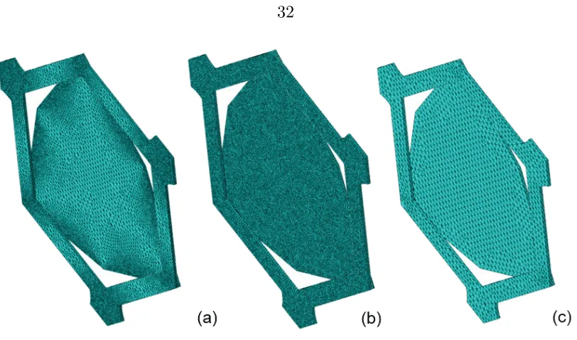
Figure 3.6 Unit cells used in my 3D FEM mesh convergence analysis. The optimized mesh, ultimately used in the model, (a) contains 66,489 nodes and 37418 elements for the frame part and 80,740 nodes and 45,169 elements for the plate part; the most refined mesh (b) contains 72,518 nodes for the frame part and 41,662 elements and 137,873 nodes and 81,331 elements for the plate part; the least refined mesh (c) contains 8,706 nodes and 3,972 elements for the frame part and 13,787 nodes and 6,776 elements for the plate part. All elements are quadratic C3D10. ... 32
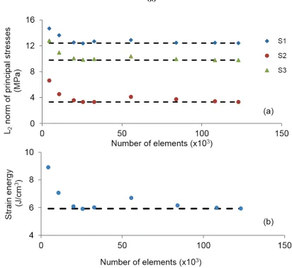
Figure 3.7 Comparison of the L2 norms of (a) principal stresses and (b) strain energy as a
function of increasing mesh density. In panel (a) the blue rhomboidal symbols represent the maximum principal stress, the red circular symbols represent the middle principal stress, and the green triangular symbols represent the minimum principal stress. Convergence to a discretization independent value is observed in principal stresses and strain energy for a sufficiently dense mesh. ... 33
Figure 3.8 (a) Simulated structure designed to be consistent with the assumption of truss-members and exhibit only in-plane behavior; (b) structure in which the outer material (shown in red) is designed to behave like a truss-member, but the inner material behaves like a plate. The only difference between the structure in (a) and in (b) is the geometry of the inner constituent shown in blue. ... 34
Figure 3.10 Deflection, δ, of a bimetallic strip of length L, and radius of curvature ρ. ... 37
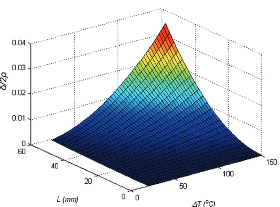
Figure 3.11 Ratio of bimetallic strip deflection δ and twice the radius of curvature ρ for a range of values of bimetallic strip length L and change in temperature ΔT. The assumption 2𝜌𝜌𝜌𝜌 ≫ 𝜌𝜌2 remains accurate over the range of values shown. ... 38
Figure 3.12 Comparison between linear FEM, nonlinear FEM, and the bimetallic strip theory for the deflection of a low CTE unit cell normalized by its thickness. Linear FEM is a good approximation until at least ΔT = 80oC, while the bimetallic strip
theory provides an upper bound for the deflection. ... 39
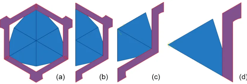
Figure 3.13 (a) Full unit cell model; equivalent unit cell model leveraging two-fold (b), three-fold (c), and six-fold (d) symmetry. ... 40
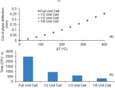
Figure 3.14 Comparison between modeling a full unit cell and its symmetric equivalents in (a) out-of-plane deflection; and (b) computational time. ... 41
Figure 3.15 (a) Fabricated low CTE sample comprised of an Al inner plate and a Ti outer frame. (b) Laser-welded interface between the sample’s Al and Ti part. ... 43
Figure 3.16 Magnitude of in-plane deformation predicted for a 70oC change in temperature
by (a) planar FEM, (b) 3D FEM, and (c) experimentally observed between 55 oC
and 125 oC. Colder color tones represent regions of the unit cell with low thermal
expansion. ... 45
Figure 3.17 CTE of Ti, Al, and unit cell samples as measured by our setup. Error bars indicate one measurement standard deviation for Al and Ti. ... 46
Figure 3.18 Unit cell CTE as a function of frame width (‘y’ axis) and CTE of constituent material (‘x’ axis). The unit CTE can range from -0.5 to 1 ppm/oC ppm by
Figure 3.19 A comparison for the CTE prediction between Equation 2.7 (solid line), Equation 3.13 (dashed line), the planar FEM (triangular symbols) and 3D FEM (circular symbols) models developed in this work, and experimental results (star symbol), for various values of CTE of constituents’ ratio α2/α1. ... 51
Figure 4.1 (a) Schematic diagram showing the geometrical characteristics of a lattice. (b) Image of a lattice fabricated out of Al and Ti constituents. ... 54
Figure 4.2 Flow chart of the setup used to measure the CTE of the array samples... 56
Figure 4.3 (a) Speckle image of array composed of Kovar and aluminum during testing; (b) IR camera image indicating temperature across the sample during testing. .. 57
Figure 4.4 Planck’s law (Equation 4.1) plotted for various temperatures; the spectral radiance is a measure of the intensity of radiation... 58
Figure 4.5 Combined effect on CTE error (%) due to measurement error in displacement and temperature. ... 60
Figure 4.6 Array schematic showing segments used to measure the CTE of an array. Measurements were made across solid lines in order to determine the thermal behavior inside the array. Dotted lines indicate areas measured to determine the overall CTE. ... 61
Figure 4.7 Strain (ppm) against temperature (oC) data for (a) Kovar/Al array and (b)
Ti/Al array along points on a sample. The points represent experimental measurements and the lines indicate linear fits of the data. The slope of the lines corresponds to the CTE. Points on the frame nodes were used for the Kovar/Al array and points on the low CTE plate nodes were used for the Ti/Al array. .... 63
Figure 4.8 In-plane displacement magnitude for Ti/Al metastructure under a thermal load of 125oC (a) as measured experimentally by DIC; and (b) as computed by FEM.
to increase computational efficiency. Blue areas indicate regions of zero displacement and low overall thermal expansion between those regions. Experimental (a) and computational (b) results agree very well both in the magnitude and spatial variation of the displacements across the sample. ... 65
Figure 4.9 CTE between two unit cells in Ti/Al and Kovar/Al arrays as a function of radial distance from the center of the unit cell, as computed by FEM. The CTE is computed by measuring the strain between a point on one unit cell and the reflectively symmetric point on a unit cell two cells away and dividing by the temperature difference (80 oC)... 67
Figure 4.10 Strain against change in temperature for the Kovar/Al (a) and Ti/Al (b) arrays, as predicted by FEM. Dotted lines indicate linear fits to the data. The CTE, α, is computed by the slope of the linear fit. ... 68
Figure 4.11 CTE of the Ti/Al and Kovar/Al arrays measured within and across the sample experimentally and computationally with FEM. The prediction of the model developed in Chapter 3, is also shown. The arrays perform as designed, with the Ti/Al array exhibiting near-zero CTE and the Kovar/Al array exhibiting negative CTE. ... 70
Figure 4.12 The CTE of metastructure arrays developed in this work compared with the CTE of their constituent materials and arrays developed in literature. The Ti/Al array developed here exhibits similar CTE to the one demonstrated in [23] with six times higher aspect ratio. The measured CTEs of Al and Ti agree well with literature [68]. The CTE of Kovar was reported in [76]. This work presents the first time a Kovar/Al array has been experimentally realized and shown to exhibit negative CTE. ... 72
Figure 5.2. Load vs. displacement as measured in a nanoindentation experiment for (a) Al and (b) Ti thin films. ... 80
Figure 5.3 Intensity vs. 2θ in a typical XRD measurement for (a) Al and (b) Ti thin films. A broader peak is observed on the Ti sample. ... 84
Figure 5.4 The effect of annealing on residual stress of Ti and Al thin films as a function of film thickness. Film stress is independent of thickness but becomes more tensile after annealing. ... 86
Figure 6.1 (a) Design of thin film low-CTE thin film metastructure. (b) SEM image of fabricated low-CTE metastructure after lift-off. ... 90
Figure 6.2 Process flow for fabrication of free-standing low-CTE thin film metastructure. ... 91
Figure 6.3 (a) Schematic showing fabrication process of free-standing Ti/Al thin film array. (b) SEM image (top view) of free-standing Ti/Al thin film array. A circular 10 unit cell diameter area was released from the substrate. ... 95
Figure 6.4 3D digital image correlation with a stereomicroscope to map small thermal displacement: (center) schematic of the set-up; (right bottom) a sample prepared with photoresist speckle pattern; (right top) 2D images of a sample taken from two different angles; and (left) 3D image constructed with DIC to show the out-of-plane displacement. ... 97
Figure 6.5 Experimental measurement of Si wafer CTE as a function of temperature. As expected, variability in the CTE measurement deceases when the CTE is computed at temperatures greater than 45 oC. ... 97
LIST OF TABLES
Table 2.1 Average CTE over measured temperature for various low and negative CTE
oxides. ... 11
Table 3.1 CTE of common pure metals [68] ... 27
Table 3.2 Correlation coefficient between unit cell CTE and design parameters. ... 49
Table 3.3 CTE of metastructures with different constituent materials ... 51
Table 4.1. CTE of arrays as experimentally measured across the entire array, between adjacent nodes on the frame constituent, and between adjacent nodes on the plate constituent. Reported errors are either one measurement standard deviation or the measurement accuracy as determined in section 4.1.3, whichever is higher. ... 64
Table 4.2 Properties of materials used in array FEM model ... 65
Table 4.3 CTE of arrays as computed by FEM between the entire array, between adjacent nodes on the frame constituent, and between adjacent nodes on the plate constituent. Since the CTE is not constant within the array, one standard deviation of the CTE between the points used to determine the CTE is also shown. ... 69
Table 5.1 Mean elastic modulus of as-deposited thin films measured by nanoindentation. 55 indentations were performed on three Al films and 30 indentations on three Ti films. Variability indicates one standard deviation. ... 81
Table 5.3 Summary of characterization of Al and Ti thin films. The thin films were used as constituent materials of the Ti/Al low-CTE metastructure. ... 87
Chapter 1
INTRODUCTION
Thermal expansion is usually considered an intrinsic material property not dependent on geometry. In this thesis, we demonstrate the ability to engineer high aspect ratio material ensembles that exhibit desired thermal expansion beyond the bounds of their constituents. We design, fabricate, and characterize material ensembles that exhibit near-zero and negative coefficients of thermal expansion (CTE) in thin foil and thin film scales, a combination which has not been demonstrated before.
characterizing these metastructures, we demonstrate that a breadth of CTEs outside the limits of the CTE exhibited by available materials can be attained. This thesis focuses on the development, characterization, and application of thin metastructures with tailored CTE. We expound upon the physical principles describing CTE tunability and characterize metastructure unit cells and arrays in thin foil and thin film size scales. We establish an experimental setup to characterize the thermal behavior of these metastructures and develop a computational model to predict and explain their unique behavior. We further develop a robust fabrication procedure to experimentally realize near-zero and negative CTE metastructures in previously unachievable scales.
1.1 Applications for Metastructures with Engineered CTE
improved performance and lower failure rates has given rise to demand for materials with low and tunable CTE.
To meet this demand, various materials have been used. Zerodur, a lithium aluminosilicate glass-ceramic trademarked by Schott Glass Technologies, and other glasses have been used for large telescope mirrors thanks to their low CTE (0 - 2 ppm/oC) [19]. In silicon integrated chips (IC’s), silicon, aluminum nitride, and silicon carbide have been used to match the CTE of the IC to prevent thermal-stress induced cracking [15]. Invar (nickel iron alloy Fe64Ni) and other nickel alloys are used in a variety of applications where thermal stability and toughness is desired. Carbon composites, which exhibit low CTE, have applications ranging from automotive to aerospace. Despite their widespread use, however, these materials exhibit several limitations: ceramics are brittle; the CTE of nickel alloys tends to vary significantly with temperature; composites are prone to thermal fatigue and are usually costly.
shown negative CTE metastructures; fabrication techniques have limited applicability to large structures; the effect of structural design parameters is not well understood; and out-of-plane deformations have not been thoroughly studied.
1.2 Thesis Objectives
In this thesis, we aim to extend scientific understanding in the field of metatsructures with near-zero and negative CTE by:
(i) Designing and experimentally realizing low and negative CTE metastructures
(ii) Extending the fabrication limits of these metastructures to thin foils and thin films
(iii) Elucidating scientific principles governing the mechanics of these metastructures
(iv) Predicting the thermal behavior of these metastructures through computational modeling
(v) Leveraging the understanding of the thermal deformation mechanics of these metastructures to develop an accurate predictive model of their CTE.
1.3 Definition of CTE for Metastructures
expand when they undergo a positive temperature change. Mathematically, the coefficient of thermal expansion (CTE) tensor, αij, is the temperature derivative of
the strain tensor, eij, under constant pressure [24]:
𝑎𝑎𝑖𝑖𝑖𝑖 =�𝜕𝜕𝑒𝑒𝜕𝜕𝜕𝜕𝑖𝑖𝑖𝑖�𝑝𝑝. (1.1)
Of course, the true strain tensor (with reference to the deformed configuration where ui is the deformation tensor) and Cauchy strain tensor, εij are defined as:
𝑒𝑒𝑖𝑖𝑖𝑖 = 12�𝜕𝜕𝑢𝑢𝜕𝜕𝑥𝑥𝑖𝑖
𝑖𝑖+
𝜕𝜕𝑢𝑢𝑖𝑖
𝜕𝜕𝑥𝑥𝑖𝑖 −
𝜕𝜕𝑢𝑢𝑘𝑘
𝜕𝜕𝑥𝑥𝑖𝑖
𝜕𝜕𝑢𝑢𝑘𝑘
𝜕𝜕𝑥𝑥𝑖𝑖� and 𝜀𝜀𝑖𝑖𝑖𝑖 =
1 2�
𝜕𝜕𝑢𝑢𝑖𝑖
𝜕𝜕𝑥𝑥𝑖𝑖+
𝜕𝜕𝑢𝑢𝑖𝑖
𝜕𝜕𝑥𝑥𝑖𝑖�. (1.2)
My work will focus on small deformations and thus from this point “strain” will refer to the Cauchy strain, εij. By assuming a linear dependence of strain on
temperature (which is accurate for small temperature changes, around non-cryogenic temperatures [24]) we can write:
𝑎𝑎𝑖𝑖𝑖𝑖 = 𝜀𝜀𝛥𝛥𝜕𝜕𝑖𝑖𝑖𝑖. (1.3)
Ignoring shear strains, we can compute the CTE along a particular direction using the following expression:
𝑎𝑎= 𝑙𝑙𝑓𝑓−𝑙𝑙𝑖𝑖
𝑙𝑙𝑖𝑖
1
𝑇𝑇𝑓𝑓−𝑇𝑇𝑖𝑖. (1.4)
This definition of CTE is applicable and useful when defining thermal expansion between atoms in a crystal. In this way, we use this definition of CTE to characterize the thermal response of metastructures. In the same way that atomic unit cells are building blocks for crystals, structural unit cells are building blocks for metastructures. The CTE of metastructures is thus defined discreetly, between nodes of unit cells within the metastructure.
1.4 Thesis Organization
Chapter 2
BACKGROUND
2.1 Thermodynamic Foundations of Thermal Expansion
Scientific explanations of thermal expansion were initially formulated by Mie and Gruneisen in the early 1900s [31-34]. Based on their work the volumetric CTE, 𝑎𝑎𝑉𝑉,
can be derived from thermodynamic principles:
aV =γCVVχΤ =γCVpχs, (2.1)
where 𝛾𝛾 (Gruneisen’s parameter) is a parameter relating the volume of a lattice to its vibrational frequency, 𝐶𝐶𝑉𝑉 and 𝐶𝐶𝑝𝑝 are the heat capacities at constant volume and
pressure, 𝜒𝜒𝜕𝜕 and 𝜒𝜒𝑠𝑠 are the isothermal and adiabatic compressibilities (bulk
moduli), and V is the lattice volume. Equation 2.1 provides an intuitive understanding of CTE as the effect of the nonlinearly dependent force experienced by an atom as a function of displacement from its equilibrium position as through Gruneisen’s parameter:
γ= −∂ln (ωi)
∂ln (V), (2.2)
where 𝜔𝜔𝑖𝑖 is the ith vibrational mode frequency. Equation 2.2 vanishes when the
atomic force-displacement relation is linear; no dependence of vibrational frequency of volume is observed in that case.
low or negative CTE exhibited by certain materials. Furthermore, it is often difficult to compute Gruneisen’s parameter from first principles without significant simplifications. Later work on the understanding of thermal expansion has focused on accurately computing Gruneisen’s parameter and generalizing the same principles to take into account non-vibrational effects and anisotropy [24]. These principles have been used to explain the low or negative CTE exhibited by certain materials.
Sections 2.2 and 2.3 review the scientific background behind commonly found low/negative CTE materials (< 2 ppm/oC) and metastructures.
2.2 Low and Negative CTE Materials
Most low CTE materials discovered so far are either ceramics or metal alloys [1, 2]. While advances in polymer technology have enabled the engineering of relatively low in-plane CTE (~4 ppm/oC) polyimide films, this comes at the cost of high out-of-plane CTE [35, 36]. Sections 2.2.1 and 2.2.2 review scientific background on low-CTE ceramics and metal alloys respectively.
2.2.1 Oxide Ceramics
Material Average CTE (ppm/oC) Temperature range (oC)
β-Spodumene 0.9 25-1000
β-Eurocryptite -6.2 25-1000
Cordierite 1.4 25-800
NZP 0.6 25-1000
NaZr2P3O12 -0.4 25-1000
Nb2O5 1.0 25-1000
Al2TiO5 1.4 25-800
Zr2P2O9 0.4 25-600
Be3Al2Si6O18 2.0 25-1000
SiO2 0.5 25-1000
Zerodur 0.12 20-600
Table 2.1 Average CTE over measured temperature for various low and negative CTE oxides.
Zerodur (CTE = 0.12 ppm/oC), a glass ceramic produced by Schott, has been widely applied as a mirror in large telescopes, such as Keck I and Keck II. Its composition is ~70% crystalline and ~30% amorphous. The CTE highly depends on the phase ratio. The crystalline and amorphous phases exhibit negative and positive CTE, respectively. The low CTE behavior of Zerodur is thus enabled by appropriately controlling the two phases to balance the overall CTE. This is a significant advantage as the CTE of Zerodur can be engineered depending on the phase ratio.
The crystalline phase exhibits negative CTE with a similar mechanism to β-Spodumene (CTE = 0.9 ppm/oC), β-Eurocryptite (CTE = -6.2 ppm/oC). These oxides exhibit very strong bonds in three dimensions and atomic structures which accommodate thermal energy in gaps within the crystal [37-39].
Secondly, as most ceramics, Zerodur is brittle. This severely limits its applicability when considering thin sheets (e.g., usually an aspect ratio between diameter and thickness of at most four is maintained for solid Zerodur substrates) [40, 41].
2.2.2 Transition Metal Alloys and Invar
Metals usually exhibit CTE one order of magnitude higher than ceramics. However, a specific set of transition metal alloys has been shown to exhibit very low CTE and unique elastic properties. The most well-known of these alloys, Invar, was discovered in 1897 by Guillaume who, for this discovery, was awarded the 1920 Nobel prize in physics [42]. This Fe65NixMn35-x face-centered cubic alloy (for x = 35) gained its name due to its approximate dimensional invariance under temperature change [24].
Depending on the nickel composition of the alloy, Invar’s CTE can range from ~0.5 to ~20 ppm/oC. Common grades (35% nickel) usually exhibit CTE of ~1.2 ppm/oC though grades designed for CTE of 5.3 ppm/oC are also developed for electronics packaging components. Invar’s CTE is an order of magnitude below what is predicted by the Gruneisen model [43, 44]. The explanation for Invar’s low CTE is related to ferromagnetic phases that occur when the nickel concentration is ~35%. Various specific mechanisms to explain this phenomenon have been proposed, however, none so far succeed in describing Invar’s unique behavior comprehensively [45-48].
thorough characterization and advances in manufacturability. However, the applicability of Invar is limited by physical principles. Invar’s CTE is roughly invariable over a small temperature range (4 to 38 oC) and substantially diminishes in temperatures higher than 100 oC due to loss of ferromagnetism as the Curie temperature (225 oC) is approached. Invar also tends to exhibit creep behavior and has a high tendency to oxidize [14, 50, 51]. The small temperature range of Invar’s low CTE has significantly limited its use in aerospace and other applications where high temperature ranges cannot be avoided.
2.3 Material Ensembles with Low or Negative Thermal
Expansion Coefficient
Material ensembles, such as certain fiber composites and low-CTE metastructures exhibit low CTE thanks to their structure and constituent materials. The low-CTE of fiber composites is usually due to the low CTE of the fiber material; for low-CTE metastructures, structural design enables low-CTEs outside the bounds of the constituent materials.
2.3.1 General Two-Phase Materials and Fiber Composites
modulus [55]. While it can be shown that for three-phase composites (such as the metastructure studied here) it is not possible to find exact expressions relating bulk modulus to thermal expansion, bounds on the CTE can be developed [56, 57]. The tightest bounds for the CTE and biaxial stiffness of composites as a function of area fraction were developed by Gibiansky and Torquato [56]. These bounds demonstrate that the ensemble CTE need not be bounded by the CTEs of its constituents but also obviate the trade-off between biaxial stiffness and CTE. Carbon-fiber reinforced composites, a particular type of composite materials, are widely used in commercial, high-end automotive, and aerospace applications thanks to their high specific strength and stiffness. In addition to those properties, carbon fiber composites can also exhibit near-zero CTE due to the negative in-plane CTE of graphite. The overall CTE of the composite is usually anisotropic and depends on the volume fraction, type of matrix, and heat treatment. It usually ranges between ~0-2 ppm/oC for carbon fiber composites. However, carbon fiber composites experience two important limitations: (i) they are prone to thermal fatigue and delamination due to the CTE mismatch between fiber and matrix and (ii) the mechanism resulting in low-CTE for fiber composites limits the lower bound of the CTE to that of the fiber.
2.3.2 Low-CTE Metastructures
schematics of the low-CTE metastructure designs developed by Lakes (a) and Steeves (b).
The design by Lakes (Figure 2.1a) uses a series of bimaterial strips which undergo bending when experiencing temperature change. Bending causes an effective contraction in unidirectional length with the expansion in the normal direction accommodated by open space.
Figure 2.1 (a) Metastructure with unbounded CTE designed by Lakes [21]. (b) Metastructure with low CTE designed by Steeves et al. [22]. High and low CTE materials are indicated by blue (darker) and orange (lighter) colors, respectively.
The curvature, κ, of a bimaterial beam as a result of thermal bending can be computed by [21, 59, 60]:
κ= 6(α2−α1)
(h1+h2)
ΔT�1+h1h2�2
3��1+h1h2�2�+�1+h1h2E1E2���h1h2�2+h2E2h1E1�, (2.3)
ε= �12cot�θ2� − 1θ�larc dκ, (2.4)
where larc is the length of a bimaterial beam or arc and θ is the included angle.
Thus the CTE, α, can be expressed as:
α= larc
(h1+h2)
6(a2−a1)�1+h1h2� 2
3��1+h1h2�2�+�1+h1h2E1E2���h1h2�2+h2E2h1E1�� 1 2cot�
θ 2� −
1
θ�. (2.5)
By manipulating the geometric and material parameters in Equation 2.5, arbitrarily high and low values of CTE can be achieved. Whether the CTE is positive or negative depends on the placement of constituents within each bimaterial beam (the metastructure shown in Figure 2.1a exhibits negative CTE). This metastructure exhibits 2D cubic symmetry which results in isotropic thermal expansion but anisotropic elasticity. However, hexagonal, elastically isotropic metastructures can also be designed with the same principles. The main advantage of this design is that it can achieve theoretically unbounded CTE.
However, the design proposed by Lakes [21] has not yet been experimentally realized. Jefferson et al. [58] patented the design and analysis of a very similar structure to Lakes’, though it is not mentioned whether that structure has been experimentally realized. The main limitation of this design is that it is dominated by bending, and thus exhibits low in-plane stiffness and strength which limits manufacturability.
The main advantage of this algorithm is that it describes a general approach to design any bimaterial structure for a set of properties, as long as the cost function can be defined. Using this methodology, Sigmund and Torquato optimized the geometry for bimaterial metastructure designs which exhibit zero and negative CTEs as well as high biaxial stiffness. However, a significant limitation of this approach is that the resulting designs tend to be too complicated for manufacturing. Additionally, the optimization algorithm is prone to falling into local minima, so it is important to test a variety of initial guesses. Another limitation is that the approach can optimize for geometry or material properties, but not for both.
More recently, Steeves et al. and Berger et al. [22, 23, 29, 30] showed that through another periodic arrangement in a two-dimensional truss-like structure of two pin jointed materials with different CTEs (Figure 2.1b) the overall response of the metastructure can exhibit zero CTE. The CTE, α, of a pin-jointed metastructure can be easily derived:
α= α1
1−12�α2α1� sin(2θ)�√31+tan (θ)�
1−21sin (2θ)�√31+tan(θ)� . (2.6)
In Equation 2.6, subscripts 1 and 2 denote materials 1 and 2, α denotes the material CTE and θ denotes a characteristic design angle. Equation 2.6 assumes that members undergo only axial stresses. This assumption limits the applicability of Equation 2.6 to slender beams.
With a few more calculations the CTE for a metastructure with bonded joints can be derived [61]:
α= α1�1−
(C1tan(θ)�sin(2θ)+√3 cos(2θ)�−12�cos(θ)+√3 sin(θ)2��a2a1−1�
where 𝐶𝐶1 =𝐴𝐴1𝑙𝑙1
2
𝐼𝐼1 and A denotes the area, E, the elastic modulus, l1 the side length of material 1, and I, the second moment. Equation 2.7 takes into account bending stresses in material 1 but not in material 2.
Equations 2.6 and 2.7 perform well for metastructures in which material 1 (blue/dark in Figure 2.1) exhibits low width to length ratio. However, when the thickness to length ratio increases the analytical predictions deviate significantly (up to ~ 200% error in this work) from FEM results. This effect is also observed in [61] and is attributed to incorrect effective length estimation of the frame. To achieve better agreement with FEM results scaling factors are used in [61].
Steeves et al. and Berger et al. [22, 23] also provide expressions for the biaxial stiffness, Sb, (such that 𝑆𝑆𝑏𝑏 =𝑁𝑁𝜀𝜀𝑏𝑏, where Nb is the force applied) of the pin-jointed
metastructures:
Sb =
E2A2
L cos�π6+θ��3−2√3 sin(θ)sin�π6+θ��
3Q+2 sin2(θ)sin�π
6+θ� , Q =
E2A2
E1A1. (2.8)
Equation 2.8 is shown to fall closely within the Gibiansky-Torquato [56] bounds for the area fraction of a three-phase system (two materials and gaps) when the biaxial stiffness is prescribed. The closeness to this bound suggests that, from a stiffness perspective, this may be an optimal design. Steeves et al.’s and Berger et al.’s design performs comparably against this bound to the designs obtained with shape optimization by Sigmund and Torquato [20, 28].
behavior was characterized computationally [23, 29]. Detailed design principles were also developed [23].
Chapter 3
ENGINEERED THERMAL EXPANSION
METASTRUCTURE UNIT CELLS
In this chapter, we study the design and testing of thin (< 200 μm), tunable CTE unit cells with large aspect ratios (~100) [62]. These unit cells can be periodically arranged to 2D arrays. Such structures are well suited for applications where low thickness, high aspect ratio, and mechanical flexibility are desirable, such as biomedical devices, solar energy systems, and semiconductors. The large aspect ratio of the metastructures in my design causes sensitivity to stress concentration. To manage these stresses we add curvature to the unit cell in the areas close to the low CTE points. We model the metastructures using both planar and full three-dimensional finite element models to guide the design of the materials’ interfaces and to inform the experiments. In order to design a thin and thermally stable unit cell we draw inspiration from previous theoretical work [22] as a starting point and employ FEM simulations to drive the design process. In 2007, Steeves et al. [22] showed that through a specific periodic arrangement in a two-dimensional truss-like structure of materials with different CTEs (Figure 3.1a) the overall response of the structure could have zero CTE at specific points. The thermal expansion of these points is governed by Equations 2.6 and 2.7, for pin-jointed and bonded structures, respectively.
vanishes for pairs of values of θ and α2/α1. Thus by designing a unit cell with specific angle θ and picking appropriate constituent materials, it is possible to create unit cells, and consequently full-scale lattices having a final CTE less than that of either constituent.
Figure 3.1 (a) Pin-joined structure designed by Steeves [22] consisting of a high and a low CTE material and exhibiting low overall CTE, governed by Equation 2.6. (b) Equation 2.6 plotted for various values of α2/α1 and θ showing the thermal expansion coefficient of a pin jointed low CTE structure normalized by α1. It is possible to achieve zero and even negative thermal expansion coefficients by picking appropriate combinations of CTE ratio α2/α1 and angle θ.
3.1 Design of Unit Cells with Engineered Thermal Expansion
constituents are lap-jointed and ultimately fabricated by spot laser-welding instead of press fit jointed as in [23].
Figure 3.2 (a) Schematic diagram showing the geometrical characteristics of the unit cell’s outer frame. θ is the angle between the internal unit cell frame angle and the inscribed equilateral triangle. (b) Schematic diagram of the unit cell’s inner plate. (c) Schematic diagram of the assembled unit cell.
[image:40.612.155.495.156.269.2]scalability to lower scales we chose to fabricate low-CTE metastructures with the dimensions shown in Figure 3.2.
3.2 Computational Study
To understand the behavior of these structures, predict their thermal and mechanical response, and improve upon previous theoretical work, we built realistic FEM models. While previous theoretical and computational work [22, 23] allows for an approximation of the thermal response, it is based on several limiting assumptions: (i) parts are composed of truss members; (ii) the interfaces are point contact; (iii) the interfaces are either pinned or bonded; (iv) it does not take into account out-of-plane effects which are relevant for this design. In addition, it gives little insight into the response of the structure as a function of variables other than θ and α2/α1. The FEM models developed in this work address the analytical limitations of previous work and enable a sensitivity analysis to material and geometric variables.
3.2.1 FEM Model Formulation
To predict the thermal response of the unit cells designed, we developed planar and full 3D FEM models of the unit cell, using commercial software Abaqus FEA [65]. The mechanics of the unit cell are modeled using static linear elastic analysis. This assumption is accurate for small deformations and linear elastic materials. The validity of this assumption is shown in section 3.2.4. In the model used here, the FEM solves the equilibrium equation by converting it to its weak form and discretizing over elements to arrive to the following formulation for my problem [66]:
w {∑ne=1(Ked−fe)} = 0 ∀w. (3.1)
In Equation 3.1, the weight function, w, is an arbitrary function which vanishes on the zero displacement boundary of the problem; d is the nodal displacement matrix and subscript e refers to a specific element. Ke and fe are the element stiffness
matrix and element external force matrix, respectively:
Ke =∫ΩeBeTDeBedΩ, (3.2)
fe = ∫ ΝΩ eTbdΩ+∫Γet NeTt dΓ
e . (3.3)
In Equation 3.2, Ω is the geometric volume of the element, B is the strain-displacement matrix, computed by taking the gradient of the shape functions N, t is the traction boundary condition specified by the problem, and Γt is the boundary
on Ω on which the traction boundary condition is applied. The displacement boundary condition is naturally applied through the shape functions.
assigned to be traction-free by default. Abaqus FEA then defines the stiffness and external force matrices per Equations 3.2 and 3.3 and solves the problem of Equation 3.1 for the nodal displacements, d, using Newton’s method [67]. The strain and stress can be computed from the displacement field and constitutive law, respectively.
As with any computational approach, it is important to identify and quantify sources of error in the solution. The major sources of error in an FEM model are of three kinds: (i) due to discrepancies between the model and the physical world; (ii) due to the inherent approximation of discretization in the model; (iii) due to compounding error during arithmetic operations in the solution phase.
Error arising from discrepancies between the model and reality is discussed in the sensitivity analysis section, 3.4. Inaccuracies arising due to discretization can be minimized by selecting an appropriate mesh and are discussed in section 3.2.3 along with a detailed mesh convergence study. Errors of the third kind are generally related to the solver of the FEM software as well as the condition of the problem being studied. In a linear elastic problem, these errors are generally small, will generally not compound, and may produce a consistent (but not growing) discrepancy with the exact solution [66]. Since the problem being studied is linear elastic and the Abaqus FEA software solver has been studied extensively this type of error is not analyzed in depth here.
and are modeled as bonded by using tie constraints in Abaqus. This method was used to simulate the way that the two parts would be joined experimentally; i.e., by welding.
Material CTE (ppm/oC)
Aluminum 23.1
Beryllium 11.3
Gold 14.2
Iron 11.8
Lead 28.9
Magnesium 24.8
Nickel 13.4
Tantalum 6.30
Titanium 8.60
Zinc 30.2
[image:45.612.217.431.99.277.2]Zirconium 5.70
Table 3.1 CTE of common pure metals [68]
3.2.2 Computational Results
Figure 3.3 The CTE of the unit cell as predicted by FEM for various CTE ratios α2/α1. The solid line indicates the prediction of Equation 2.7. The circular, triangular, star, and rhomboidal symbols indicate the FEM prediction of a unit cell design with frame width ratios of 3.84x10⁻², 5.44x10⁻², 6.56x10⁻², and 10.97x10⁻², respectively. The square symbols indicate the planar FEM prediction of the 6.56x10⁻² frame width ratio unit cell. The full 3D solid FEM model predicts a higher CTE for the unit cell than the planar FEM model.
response of a metastructure consisting of all beam elements (as in the theoretical framework) and of one with a plate interior constituent, using FEM. Detailed analysis shown in section 3.2.3 yielded negligible difference in the thermal response of the two unit cells.
Figure 3.4 Isometric view of the shape of an exemplary unit cell as predicted by planar (a) and 3D (b) FEM with an 80 oC thermal load. Contours show the magnitude of the displacement vector. The out-of-plane deformation predicted by the 3D FEM case is evident in panel b. Displacements are magnified 40 times in (b).
deformation increases, exhibiting the importance of out-of-plane effects at thinner scales.
Figure 3.5 (a) The maximum out-of-plane deformation of a unit cell as a function of the unit cell’s thickness. The maximum out-of-plane deformation occurs at the frame’s low CTE points. (b) The CTE of a unit cell as a function of the unit cell’s thickness. There is a measurable decrease in the CTE as the thickness decreases.
Figure 3.5b shows the effect of thickness on the CTE of the unit cell. As the thickness increases from 50 μm to 250 μm the CTE also increases, from 0.92 to 1.49 ppm/oC. The dependence of CTE on thickness suggests that the out-of-plane deformation has a measurable impact on the CTE of the metastructure. However, this impact is small and does not influence the low-CTE performance of the metastructure.
3.2.3 Mesh Convergence and Comparison with the Theoretical Solution
converges to a value independent of discretization choice. For this study, we modeled the response of a unit cell under a thermal load of 80 oC. Models were made with increasing mesh densities using quadratic C3D10 elements. Quadratic elements provide a one order of magnitude lower error for a given element size compared to linear elements [66]. Once a convergence was achieved the mesh was optimized by lowering the mesh density in areas of low stress to increase computational efficiency, resulting in the mesh shown in Figure 3.6a.
Figure 3.6 Unit cells used in my 3D FEM mesh convergence analysis. The optimized mesh, ultimately used in the model, (a) contains 66,489 nodes and 37418 elements for the frame part and 80,740 nodes and 45,169 elements for the plate part; the most refined mesh (b) contains 72,518 nodes for the frame part and 41,662 elements and 137,873 nodes and 81,331 elements for the plate part; the least refined mesh (c) contains 8,706 nodes and 3,972 elements for the frame part and 13,787 nodes and 6,776 elements for the plate part. All elements are quadratic C3D10.
The L2 norm of the principal stresses and the strain energy over the entire volume was used as the metric to quantify mesh quality. The L2 norm of a function is a way of defining the magnitude of a function f(x) and is given by:
‖𝑓𝑓(𝑥𝑥)‖𝐿𝐿2 = �∫ 𝑓𝑓2(𝑥𝑥) 𝑑𝑑𝑥𝑥
𝑥𝑥2
𝑥𝑥1 �
1/2
. (3.4)
Figure 3.7 Comparison of the L2 norms of (a) principal stresses and (b) strain energy as a function of increasing mesh density. In panel (a) the blue rhomboidal symbols represent the maximum principal stress, the red circular symbols represent the middle principal stress, and the green triangular symbols represent the minimum principal stress. Convergence to a discretization independent value is observed in principal stresses and strain energy for a sufficiently dense mesh.
[image:51.612.110.522.81.459.2]assumptions (Equation 2.7). While a thorough discussion of these assumptions is presented in section 2.3.2, the three most relevant assumptions are: (i) structural elements behave like rods; (ii) the contact area is of infinitesimal size; and (iii) the structure undergoes purely in-plane deformation. To test the validity of my FEM model we modified the structure and model parameters in order to meet the three assumptions. Figure 3.8a shows the unit cell simulated to verify the FEM’s model accuracy. While the basic design was kept the same, features that could cause deviation from the theoretical result were removed and all structural elements were designed in order to behave like truss members (assumption i).
Figure 3.8 (a) Simulated structure designed to be consistent with the assumption of truss-members and exhibit only in-plane behavior; (b) structure in which the outer material (shown in red) is designed to behave like a truss-member, but the inner material behaves like a plate. The only difference between the structure in (a) and in (b) is the geometry of the inner constituent shown in blue.
the same plane. The CTE of the unit cell was measured for various ratios of CTE constituents by performing a similar analysis as in 3.2.1. In addition, the effect on thermal response of the inner constituent being a plate, as opposed to a rod (which the theory assumes) was assessed by computing the CTE of the unit cell shown in Figure 3.8b. Figure 3.9 shows the comparison between theoretical predictions of the CTE and the FEM model developed in this work. Excellent agreement is observed between the theory for bonded parts and the model. It is also evident that changing the inner constituent (shown as blue in Figure 3.8) from a rod to a plate does not significantly influence the CTE of the unit cell.
Figure 3.9 Comparison between theoretical predictions of the unit cell CTE as a function of CTE of constituents’ ratio and FEM model developed in this work. The solid line corresponds to a theory assuming pin-jointed structures, while the dashed line shows the theory for bonded structures. The FEM predictions for a structure with rod-like members and a structure with plate-like inner constituents are shown with blue asterisks and red circles, respectively.
-4 -2 0 2 4
1.70 1.80 1.90 2.00 2.10 2.20 2.30 2.40
Un it ce ll CT E (p pm / o C)
CTE of constituents' ratio, α2/α1
In fact, when the inner constituent can be assumed to behave like a plate, the CTE of the overall structure is slightly lower than when it behaves like a rod. This can be attributed to the increased stiffness of the plate.
The excellent agreement between the theory and the model when the model is simplified to the theoretical limits confirms the viability of the FEM model in this work and enables predictive use of this model.
3.2.4 Validity of the Linearity Assumption
The model developed in this work and formulated in section 3.2.1 assumes linearity, i.e., the response is a linear function of the input variable over the range of interest. This assumption is valid when the material constitutive law is linear and when deformations are “small”. In this work, material properties are assumed linear over the range of interest. To verify that displacements are indeed small, theoretical and computational analyses were performed.
For the theoretical analysis, the unit cell was assumed to behave like a bimetallic strip. It can be shown that the curvature, κ, of a bimetallic strip under thermal loading is expressed by [59]:
𝜅𝜅= 1𝜌𝜌= 4833(𝛼𝛼2−𝛼𝛼1)(𝛥𝛥𝑇𝑇)
ℎ . (3.5)
In Equation 3.5, α2 and α1 are the CTEs of two materials, h is the thickness of the
Figure 3.10 Deflection, δ, of a bimetallic strip of length L, and radius of curvature ρ.
Thus the deflection δ is expressed by:
𝜌𝜌(2𝜌𝜌 − 𝜌𝜌) = �𝐿𝐿2�2. (3.6)
This expression can be linearized to 𝜌𝜌= 8𝜌𝜌𝐿𝐿2 provided that 2𝜌𝜌𝜌𝜌 ≫ 𝜌𝜌2; i.e., the
deflections are small compared to the radius of curvature. To test this linearity assumption we compare 2𝜌𝜌 and 𝜌𝜌. We can compute δ by solving 3.6 for δ:
𝜌𝜌= 2𝜌𝜌±�4𝜌𝜌2 2−𝐿𝐿2. (3.7)
Figure 3.11 Ratio of bimetallic strip deflection δ and twice the radius of curvature ρ for a range of values of bimetallic strip length L and change in temperature ΔT. The assumption 2𝜌𝜌𝜌𝜌 ≫ 𝜌𝜌2 remains accurate over the range of values shown.
As Figure 3.11 shows, the assumption that 2𝜌𝜌𝜌𝜌 ≫ 𝜌𝜌2 is accurate for strip lengths
at least up to 60 mm (unit cell studied here is ~13 mm long) and temperature differences at least up to 150oC. Furthermore, the bimetallic strip assumption is a conservative (upper) estimate of the out-of-plane deflection of the unit cell since in the unit cell the two materials are not in full contact. Based on this analysis, the linearity assumption is valid for the unit cell under the conditions studied.
Figure 3.12 Comparison between linear FEM, nonlinear FEM, and the bimetallic strip theory for the deflection of a low CTE unit cell normalized by its thickness. Linear FEM is a good approximation until at least ΔT = 80oC, while the bimetallic strip theory provides an upper bound for the deflection.
The bimetallic strip theory predicts deflections between two and four times higher than the FEM and as predicted, provides an upper bound for the deflection of the unit cell studied here (Figure 3.12). By comparison with nonlinear FEM, the linearity assumption is confirmed for values up to least 80oC ΔT. The linear assumption significantly deviates (~25% error) for normalized deflections greater than 0.25. This analysis provides a more stringent bound than the convention used in industry where deflection for a plate in bending can be described as “small” when it is smaller than half the thickness of the plate [70]. In this work, nonlinearity will be assumed whenever deflections are greater than 25% of the plate thickness.
3.2.5 Symmetric Boundary Conditions on the Unit Cell
While a full 3D FEM model analyzes the exact geometry of a structure with no simplifications or artificial boundary conditions, it is often advantageous to reduce
0 1 2 3 4 5 6
0 50 100 150 200 250 300 350 400
D ef lec tion t o thi ck nes s ra tio
ΔT (oC) Linear FEM
Nonlinear FEM
the size of the problem being modeled by leveraging symmetries. The reduced model should output the same solution as the full model but at reduced computational time. The unit cell in this work exhibits two-fold, three-fold, and six-fold symmetry. Figure 3.13 shows the full unit cell (a) and its equivalent symmetric models (b,c,d).
[image:58.612.116.529.218.359.2]Figure 3.13 (a) Full unit cell model; equivalent unit cell model leveraging two-fold (b), three-fold (c), and six-fold (d) symmetry.
Figure 3.14 Comparison between modeling a full unit cell and its symmetric equivalents in (a) out-of-plane deflection; and (b) computational time.
3.3 Experimental Study
[image:59.612.117.520.77.387.2]3.3.1 Sample Preparation
We fabricated and prepared samples for testing in three steps: (i) fabricate the Ti frame and Al plate separately; (ii) attach the two pieces at three points; (iii) add speckle pattern for Digital Image Correlation [71, 72] testing. Frame and plates were fabricated using wire electron discharge machining (EDM). Figure 3.15a shows a unit cell after the laser welding step, but before the speckle pattern has been applied. Following fabrication the two parts were cleaned and attached at three points by laser welding (Figure 3.15b). Laser welding was performed with a 50 W maximum power pulsed Nd:YAG laser. The power and frequency were adjusted such that the laser beam melted the titanium, which has a higher melting point than aluminum (1941 K vs. 933 K), but did not go through to the aluminum. Instead, the molten titanium at the interface with the aluminum melted a region of aluminum which resulted in the weld. During the laser welding process, the laser beam was normal to the sample while Argon gas was used to remove oxygen from the weld area.
From a random sample of speckles, the average speckle size was 26.97 pixels. Approximately half of the speckles contained less than 20 pixels and 40% of speckles contained 10-20 pixels. The size was controlled by changing the distance from which black spray paint was applied. The speckle size must be large enough to prevent aliasing but small enough that the correlation algorithm can accurately track the speckle subsets.
Figure 3.15 (a) Fabricated low CTE sample comprised of an Al inner plate and a Ti outer frame. (b) Laser-welded interface between the sample’s Al and Ti part.
3.3.2 Experimental Setup
were composed of 21 pixels and the step size was five pixels. This resulted in a ~50 μm spatial resolution and a correlation displacement accuracy of ~500 nm. The correlation accuracy corresponds to ~5% of the maximum displacement observed. The 50 μm spatial resolution is adequate to capture the overall deformation behavior of the ~12 mm sample.
A similar experimental setup to the one used here is discussed in detail in section 4.1. The samples were heated on a hot plate and the temperature was measured using a thermocouple and a resistance temperature detector. Images were taken once the temperature had stabilized at steps between 40 oC and 160 οC using a Nikon ShuttlePix P-400R microscope. We then computed the displacements at each temperature step using commercial VIC-2D [73] software.
3.3.3 Measurement of the Thermal Expansion Coefficient
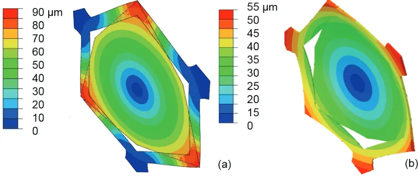
Figure 3.16 Magnitude of in-plane deformation predicted for a 70oC change in temperature by (a) planar FEM, (b) 3D FEM, and (c) experimentally observed between 55 oC and 125 oC. Colder color tones represent regions of the unit cell with low thermal expansion.
Figure 3.17 CTE of Ti, Al, and unit cell samples as measured by our setup. Error bars indicate one measurement standard deviation for Al and Ti.
3.4 Predicting and Engineering the Coefficient of Thermal
Expansion through Sensitivity Analysis
To demonstrate CTE tunability with this design, establish the effect of measurement error on our experimental results, and determine the sensitivity of the CTE to its dependent variables, we performed a sensitivity analysis on the CTE as a function of six parameters: the CTEs and elastic moduli of the constituents (α1 , α2, E1, E2) and the width of the frame (𝑓𝑓𝑤𝑤𝑖𝑖𝑤𝑤𝑤𝑤ℎ) and the size of the
Figure 3.18 Unit cell CTE as a function of frame width (‘y’ axis) and CTE of constituent material (‘x’ axis). The unit CTE can range from -0.5 to 1 ppm/oC ppm by adjusting the CTE of one of its constituents and the width of the other constituent.
of each of these variables and the unit cell CTE was computed in the following way:
r = n−11 ∑ �Xi−X
Sx � �
Yi−Y
Sy �
n
i=1 . (3.8)
In Equation 3.8, 𝑋𝑋 and 𝑌𝑌 are the sample and response means, and 𝑆𝑆𝑥𝑥 and 𝑆𝑆𝑦𝑦 are
the sample and response standard deviations, as defined in Equations 3.9 and 3.10 below:
X =1n∑ni=1Xi, (3.9)
Sx = �n−11 ∑ �Xi−X�
2 n
i=1 . (3.10)
The dataset used to compute the correlation coefficient is shown in Appendix A.2. Table 3.2 shows the correlation of unit cell CTE with the six parameters. As expected, the strongest correlation is observed with the CTEs of the constituents. However, while theoretical work predicts that the unit cell thermal expansion depends equally on the CTE of the constituents, the sensitivity analysis shows a much stronger correlation on the CTE of the frame. This is likely attributed to the finite width of the frame which the theory does not take into account. Also strong correlation of the unit cell CTE is observed on the width of the frame. The Young’s moduli of the two materials and the contact area between them do not have a strong correlation with the CTE.
α1 α2 fwidth Acontact E1 E2 0.89 -0.33 0.29 0.04 0.03 -0.05
Since α1, α2, and the frame width (fwidth) are the most important parameters influencing the CTE of this metastructure, we conducted a series of full 3D FEM simulations to determine the effect of these variables on the CTE. Statistics programming language R [75] was used to produce a multivariate fit of the CTE on those three variables. The multivariate fit performed is a linear, least squares regression and results in an expression of the unit cell CTE as a linear function of the six parameters. Give a dataset of inputs X, and response variable y, the least squares regression takes the following form:
y = Xb +ε. (3.11)
In Equation 3.11, b is computed to minimize ε and yield the coefficients linking the response variable to the input as follows:
b = (XTX)−1XTy. (3.12)
Performing the least squares calculation on the dataset shown in Appendix A.2, yields the following regression for the unit CTE:
α= −4.263 + 1.689 α1−0.646 α2+ 87.945 fwidth. (3.13)
In Equation 3.13, 𝛼𝛼1 and 𝛼𝛼2 are in ppm, 𝑓𝑓𝑤𝑤𝑖𝑖𝑤𝑤𝑤𝑤ℎ is in μm/μm, and the output α is
expressed in ppm/oC.
Figure 3.19 A comparison for the CTE prediction between Equation 2.7 (solid line), Equation 3.13 (dashed line), the planar FEM (triangular symbols) and 3D FEM (circular symbols) models developed in this work, and experimental results (star symbol), for various values of CTE of constituents’ ratio α2/α1.
Equation 3.13 was designed for the range 2.3 ≤α2/α1 ≤ 3.6. H ow ever, E quation 2 performs well at the boundary α2/α1 = 1 for α2 = α1= 23.1 (11% error) and α2 = α1= 8.6 (22% error). As seen in Figure 3.19, Equation 3.13 agrees well with computational and experimental results in this work. Using Equation 3.13 we can thus engineer the CTE of my samples by varying three parameters: the CTEs of the constituents and the width of the frame. We can use the strong sensitivity of the frame’s width to make coarse adjustments to the unit cell CTE, while making finer adjustments through the CTE of the plate and frame. This enables the design of metastructures with a precisely specified CTE.
Constituent 1 Kovar Titanium Nickel
Constituent 2 Aluminum Aluminum Aluminum CTE prediction (ppm/oC) -3.63 1.12 8.35
Table 3.3 CTE of metastructures with different constituent materials
Metastructures with a wide range of CTE can be fabricated by using the approach described in this work. Even negative CTEs can be achieved if the ratio of CTEs of the constituents is high enough as in the in the case of the metastructure composed of Kovar (α=5.9 ppm/oC) [76] and Aluminum.
3.5 Summary
Chapter 4
TAILORING THE THERMAL EXPANSION OF
HIGH ASPECT RATIO METASTRUCTURE
ARRAYS
In this chapter, we demonstrate metastructure arrays that exhibit a specified CTE which can be tailored by selecting constituent materials with difference thermal properties. The objective is to achieve arrays with large area coverage that can exhibit low and negative CTE.
The ability to vary the CTE of an array by appropriately choosing its constituent materials is demonstrated experimentally and computationally. The metastructure arrays fabricated and tested consisted of 16 unit cells with an aspect ratio of ~570. We studied the thermal response of the arrays as a whole as well as within the array. We observed excellent experimental agreement with FEM modeling and measured the CTE to be -3.72 and 1.17 ppm/oC for arrays made of Kovar/Al and Ti/Al, respectively.
4.1 Experimental
4.1.1 Sample Design and Fabrication
Arrays consisting of 16 (4x4) unit cells were designed for fabrication and testing (Figure 4.1a). The number of unit cells was chosen such that there would be sufficient area to test away from the boundaries of the unit cell to avoid potential boundary effects.
Figure 4.1 (a) Schematic diagram showing the geometrical characteristics of a lattice. (b) Image of a lattice fabricated out of Al and Ti constituents.
Previous work only studied lattices containing up to 10 unit cells and discussed the presence of boundary effects [23, 29]. Here, there exists four interior cells away from the boundary, allowing investigation of the lattice in all directions, in contrast to previous work [23].
Parts manufactured by EDM were also frequently damaged due to high temperatures on the part surface during machining. Chemical etching of the lattice constituents was performed in bulk by Photofabrication Engineering Inc [77]. This fabrication technique was essential in the successful development of arrays with engineered CTE. Analysis performed for single unit cells (Section 3.4) guided the material selection for the constituents of the arrays. Frame parts were made out of titanium and Kovar (a nickel-cobalt ferrous alloy related to Invar). All inner plates were made out of aluminum.
The constituent frames and plates were then joined by laser welding as in the unit cell. To prevent inconsistencies in the welds, tooling was designed to keep the parts in intimate contact during the process. Lack of intimate contact between the parts during welding was deemed to be the leading cause of weld inconsistency. Stress developed during laser-welding contributed to curvature in the initial configuration of the arrays, though the effect of the initial array shape was not extensively studied. Figure 4.1b shows an array successfully fabricated out of a titanium frame with aluminum inner plates. Successful arrays were also made with Kovar. The constraints in materials selection were weldability and lithographic patterning and etching.
4.1.2 Thermal Testing Methodology
Figure 4.2 Flow chart of the setup used to measure the CTE of the array samples.
thermal chamber. However, use of a thermal chamber would result in a large working distance in the optics used for digital image correlation and negatively impact resolution (see section 4.1.3). Instead, we chose to allow variability in the temperature across the sample, provided that it could be accurately determined. Accurate, full-field knowledge of the temperature across the sample was obtained with an infrared (IR) camera. Displacements were computed with DIC. Then, the CTE of the sample was computed by analyzing the displacement and temperature data. An aluminum plate on top of the hot plate was used to improve the uniformity of heating. The hot plate temperature was incrementally increased in 20-40 oC steps and the sample was let to equilibrate at each temperature for about 20 minutes. Then, samples were imaged simultaneously with two optical cameras for DIC (Figure 4.3a) and an IR camera (Figure 4.3b). DIC was used to measure the thermal displacements and the IR camera was used to measure the sample temperature.
An IR camera works by detecting electromagnetic radiation in the infrared spectrum (between 0.75 and 100 μm), which bodies at temperatures above 0 K emit. The intensity of this radiation is a function of physical constants, the absolute temperature of the body, and the wavelength of the radiation and is given by Planck’s law [78]:
Wλb = 2hc
2
λ5�ehc�λkT−1�. (4.1)
In Equation 4.1, Wλb is the spectral radiant emittance at wavelength λ of a
blackbody at temperature T, h is Planck’s constant (6.626 x 10⁻³⁴ J s), c is the speed of light (2.998 x 10⁸ m/s), and k is the Boltzmann constant (1.381 x 10⁻²³ J/K). Equation 4.1 is plotted for various temperatures in Figure 4.4.
[image:76.612.197.453.375.578.2]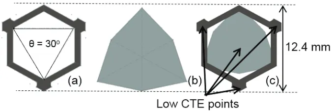
![Table 3.1 CTE of common pure metals [68]](https://thumb-us.123doks.com/thumbv2/123dok_us/8814822.919966/45.612.217.431.99.277/table-cte-common-pure-metals.webp)