Customised ensemble methodologies for deep learning: boosted residual networks and related approaches

(1)

BIROn - Birkbeck Institutional Research Online

Mosca,

Alan and Magoulas,

George (2018) Customised ensemble

methodologies for deep learning: boosted residual networks and related

approaches. Neural Computing and Applications 31 (6), pp. 1713-1731.

ISSN 0941-0643.

Downloaded from:

Usage Guidelines:

Please refer to usage guidelines at

or alternatively

(2)

Customised ensemble methodologies for Deep

Learning: Boosted Residual Networks and

related approaches

Alan Mosca? ?? _{and George D Magoulas}

Department of Computer Science and Information Systems Birkbeck, University of London

email: [email protected], [email protected]

Abstract. This paper introduces a family of new customised method-ologies for ensembles, called Boosted Residual Networks (BRN), which builds a boosted ensemble of Residual Networks by growing the member network at each round of boosting. The proposed approach combines recent developements in Residual Networks - a method for creating very deep networks by including a shortcut layer between different groups of layers - with Deep Incremental Boosting, a methodology to train fast ensembles of networks of increasing depth through the use of boosting. Additionally, we explore a simpler variant of Boosted Residual Networks based on Bagging, called Bagged Residual Networks (BaRN). We then analyse how the recent developments in Ensemble distillation can im-prove our results. We demonstrate that the synergy of Residual Networks and Deep Incremental Boosting has better potential than simply boost-ing a Residual Network of fixed structure or usboost-ing the equivalent Deep Incremental Boosting without the shortcut layers, by permitting the cre-ation of models with better generaliscre-ation in significantly less time.

1 Introduction

Residual Networks are a type of deep network recently introduced in [15], char-acterized by the use ofshortcutconnections (sometimes also calledskip connec-tions). These shortcuts link the input of a layer of a deep network to the output of another layer positioned a number of levels “above” it. As a result, each one of these shortcuts shows that networks can be built inblocks, which rely on both the output of the previous layer and the previous block. The advent of Residual Networks has allowed for the development of networks with many more layers than traditional Deep Networks, in some cases with over 1000 blocks, such as the networks in [17].

Ensembles of machine learning models have been part of the field for a long time [35,8], and have recently shown to be an efficient solution to adversar-ial learning [40] and as a vehicle for improving the single model accuracy [27],

?_{Corresponding Author} ??

(3)

II

as well as a method for creating better generalisation by consensus of mod-els. Simultaneously, ensemble methods are often left as anafterthought in Deep Learning models: it is generally considered sufficient to treat the Deep Learning method as a “black-box” and use a well-known generic Ensemble method to obtain marginal improvements on the original results. Whilst this is an effective way of improving on existing results without much additional effort, we find that it can amount to a waste of computations. Instead, it would be much better to apply an Ensemble method that is aware, and makes use of, the underlying Deep Learning algorithm’s architecture.

Such customised approaches for designing Ensembles that are specific to a particular model, allow us to improve on the generalisation and training speed compared to traditional Ensembles, by making use of particular properties of the base classifier’s learning algorithm and architecture. We follow this method-ology to design a type of Ensemble called Boosted Residual Networks (BRN), which makes use of developments in Deep Learning, previous other customised Ensemble methodologies, and combines several ideas to achieve improved results on benchmark datasets. We then build on these results to construct related vari-ations of this method, to highlight how such customised ensemble methods can be created with particular specific properties.

The version of BRN presented in this paper presents some performace im-provements over the previous version presented in [24]. The new version allows for a variant suitable for networks whose outputs are real-valued, called BRN.R, and we present a further derivation, based on Bagging [5] instead of Boosting, called BaRN.

Using a customised ensemble allows us to improve on the generalisation and training speed of other ensemble methods by making use of the knowledge of the base classifier’s previous learning, structure, and architecture. Experimen-tal results show that Boosted Residual Networks achieve improved results on benchmark datasets.

When compared with existing customised ensemble methods such as DIB [23], BRN enables the creation of almost arbitrary length models, thanks to the abil-ity of residual networks to not be affected by the common issues created by a large number of layers, such as vanishing or exploding gradients[15].

In Sections 2 through to 4 we present the prerequisite background to BRN. Section 5 presents the methodology itself. Section 6 explores an additional method based on Bagging. Section 7 analyses the application of distillation to our meth-ods and the chosen baselines. Section 8 shows the experiental results. Section 9 provides further analysis and explores potential future work.

2 Relevant techniques in Deep Learning

(4)

III

2.1 Shortcut connections in Networks

The idea of adding shortcuts connections in a network was introduced in the past in [44,22,30,4,32]. Work has been done, for example, to add a single linear layer between the input and the output of a network to simplify the learned function [32]. Other research utilises shortcut connections to address internal issues to network, such as vanishing gradients, layer responses, and propagated errors [31,36,37,41]. Highway Networks [39,38] are also a type of network that uses shortcut connections. In this case, the shortcut connection is guarded by a learned gating system, so it is no longer a simple identity function. The “infor-mation highways” created by this process are argued to enable the network to route information internally, enabling the training of deeper networks.

Dense Convolutional Neural Networks [19] are another type of network that makes use of shortcuts, with the difference that each layer block is directly connected to all its ancestor layer blocks by a shortcut link. This increases sig-nificantly the computational complexity of the network, adding training time and memory requirements to the training process.

2.2 Residual Networks

Residual Networks [15] are a particular type of Convolutional Neural Network built on the notion of connectedblocks of layers. Each block in a Residual Net-work is composed of a combination of convolutional, pooling or batch normal-isation layers. These blocks are connected to each other both in a sequential feed-forward layout, as seen in standard convolutional networks, as well as via

skip connections. Each skip connection provides a link between the output of the

final layer of a blockbito the input of a descendantbj. A skip connection is then

created for each of the descendants bi+1. . . bn, where nis the total number of

blocks in the network. These particular skip connections only connect forwards and do not form loops in the network. Residual Networks have enabled the cre-ation of very deep networks, in some cases in excess of 1000 layers [17]. This is because the technique has been explicitly created to solve the problems that are usually associated with the depth of a network.

The goal of the Residual Network is to explicitly let layers approximate a

residual function F(x) =H(x)−x, where H(x) is the true target function to

be learned. The output is then recast asF(x) +xto predict the originalH(x) again. This is based on the assumption thatH(X)−xis much easier to learn than just H(X). Early work on Residual Networks has shown that they are very good at addressing thedegradationproblem: as a network gains additional layers, it become progressively harder to learn the target function, with accuracy degrading very rapidly. It is to be noted that this is not due to overfitting (the increased error is observed on the training set as well).

(5)

IV

larger network can always be at least as good as a smaller one. This principle also supports the idea of Boosted Residual Networks, Deep Incremental Boosting, and Residual Networks, as it is crucial to be able to extend networks to an arbitrary number of layers.

2.3 Learning Additive Improvements

In the presentation of DIB [23], the notion is introduced that each new layer being added to the network is learningcorrections from the previous model. It has been shown that this principle is also applicable to Residual Networks and Highway networks [13], where each additional block can be in fact equated to a further unrolling of an iterative learning procedure. Therefore it is also shown that each new block in such networks is not necessarily learning increasingly higher level representations, but additional refinements of the estimates of the previous layers. This principle partially justifies the empirical observation that at each round of BRN (and variants), the accuracy of the single classifier improves.

2.4 Transfer of Learning in Convolutional Networks

Transfer of Learning has also had an impact on Deep Learning. For example, for Convolutional Networks, certain sub-features in the lower layers of a trained network have been shown to be entirely transferrable to a new CNN. This leads to improved training results, and much faster training compared to having train the entire network from scratch, as shown in [46]. Additionally, specific exper-imental work on computer vision dataset shows that mid-level representations are transferrable between networks trained on different dataset [29].

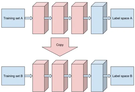
An illustration of how the early and middle layers are copied between different architectures is shown in Fig. 1

2.5 Comparison to approximate ensembles

While both Residual Networks and Densely Connected Convolutional Networks may be unfolded into an equivalent ensemble, we note that there is a differen-tiation between an actual ensemble method and an ensemble “approximation”. During the creation of an ensemble, one of the principal factors is the creation

ofdiversity: each base learner is trained independently, on variations (resamples

in the case of boosting algorithms) of the training set, so that each classifier is guaranteed to learn a different function that represents a view of the original training dataset. This is the enabling factor for the ensemble to perform better in aggregate.

(6)

V

Fig. 1: Illustration of the Transfer Learning process in Convolutional Networks: a network trained on a dataset in problem spaceA, donates the weights from its lower and middle layers to initialize a new network. This is subsequently trained on a dataset from a seemingly unrelated problem space B

Fig. 2: A Residual Network of N blocks can be unfolded into an ensemble of 2N₋_{1 smaller networks.}

(7)

VI

each underlying set of layers. We conjecture that this aggressive dimensionality reduction before the aggregation has a regularising effect on the ensemble.

3 Traditional Boosting Methods

Boosting is a technique first introduced in [34,35], by which classifiers are trained sequentially, using a subset of the original dataset, with the prediction error from the previous classifiers affecting the sampling weight for the next round. After each round of boosting, the decision can be made to terminate and use a set of calculated weights to apply as a linear combination of the newly created set of learners.

AdaBoost In [35], Freund and Schapire present two variants of boosting, called AdaBoost.M1 and AdaBoost.M2. The main difference between the two algo-rithms is in the way the final hypothesis is calculated and how multiple class problems are handled, with both variants shown in detail in Algorithhms 1 and 2. Each boosting variant builds a distribution of training set resampling weights

Dt.Dt is updated at each iteration to increase theimportance of the examples

that are harder to classify correctly. Each resampled dataset is used to train a new classifierht, which is then incorporated in the group with a weightαt, based

on its classification errort. The newDtis then generated for the next iteration.

The main differences between each AdaBoost variant lie in how the errort, the

classifier weight αt, the dataset distribution Dt and the aggregation functions

are designed and implemented.

3.1 SAMME

The original AdaBoost algorithm works very well in the binary classification set-ting. However, when the number of output classesk >2 it suffers from problems with weak classifiers with error above 1₂, which led the authors to create Ad-aBoost.M2. Another solution is presented as Stagewise Additive Modeling using a Multi-class Exponential loss function (SAMME) [14]. SAMME compensates for the fact that αwould be negative for errors above 1

2. SAMME is shown in

Algorithm 3. An in-depth study of multi-class Boosting is provided in [28]. When the base classifier outputs a real–valued probability P(k|x) rather than a one–hot encoded class decision, it may prove advantageous to utilise this additional information to calculate more precise sampling weights and improve the classifier’s output. AdaBoost.M2 is an example of an algorithm the exploits this property. A variant of SAMME for classifiers that exploits this knowledge also exists, called SAMME.R [14], shown in Algorithm 4.

4 An existing customised method: Deep Incremental

Boosting

(8)

VII

Algorithm 1 AdaBoost.M1

Inputs: training setX0, an algorithm to create classifier hypothesesh(X)

Outputs: a trained ensemble classifierH(X)

D0,i= 1/M∀i

t= 0

W0←randomly initialised weights for first classifier

whilet < tend do

Xt←sample fromX0 with distributionDt

ht←new classifier on current subset

t=P_i_:_h

t(xi)6=yiDt(i)

if t>1₂ then abort loop

end if

βt=t/(1−t)

Dt+1,i=

Dt,i

Zt ·

(

βt if ht(xi) =yi

1 otherwise |∀i= 1· |x|

whereZt is a normalisation factor such thatDt+1is a distribution

αt=_β1

t

t=t+ 1

end while

H(x) = argmax_y∈Y

PT

t=1logαtht(x, y)

Algorithm 2 AdaBoost.M2

D0,i= 1/M for alli

t= 0

whilet < tend do

t= 1₂P(i,y)∈BDt,i(1−ht(xi, yi) +ht(xi, y))

βt=t/(1−t)

Dt+1,i=

Dt,i

Zt ·β

(1/2)(1+ht(xi,yi)−ht(xi,y))_|∀_i_{= 1}_{· |}_x_|

αt=_β1_t

t=t+ 1

end while

H(x) = argmaxy∈Y

PT

(9)

VIII

Algorithm 3 SAMME

Outputs: a trained ensemble classifierH(X) setkto the number of output classes in the problem

D0,i= 1/M for alli

t= 0

whilet < tend do

t=

Pn

i=1Dt(i)I(yi6=ht(Xt)))

Pn i=1Dt(i)

αt=log1−t

t +log(k−1)

Dt+1,i=

Dt,i

Zt e

αtI(yi6=ht(Xt)))_|∀_i_{= 1}_{· |}_x_|

t=t+ 1

end while

H(x) = argmaxy∈Y

PT

t=1αtht(x, y)

Algorithm 4 SAMME.R

Outputs: a trained ensemble classifierH(X) setkto the number of output classes in the problem

D0,i= 1/M for alli

t= 0

whilet < tend do

Obtain weighted class probability estimatespi(X) =Pt(y=ci|Xt, ht), i= 1. . . k

replaceht(Xt)←(k−1)

logpi(X)−1

k

Pk

j=1logpj(X)

, i= 1. . . k

Dt+1,i=

Dt,i

Zt e

−k−1_k yTlogp(Xta)_|∀_i_{= 1}_{· |}_x_|

t=t+ 1

end while

H(x) = argmax_y∈Y

PT

(10)

IX

The method makes use of principles from transfer of learning, like for example those used in [46], applying them to conventional AdaBoost ([34]).

Deep Incremental Boosting increases the size of the network at each round by adding new layers at the end of the network. This, as discussed, is extremely unlikely to harm the learning process. In the original paper on Deep Incremental Boosting [23], this has been shown to be an effective way to learn thecorrections

introduced by the emphatisation of learning mistakes of the boosting process. The argument as to why this works effectively is based on the fact that the datasets at roundst and t+ 1 will be mostly similar, and therefore a classifier

ht that performs better than randomly on the resampled dataset Xt will also

perform better than randomly on the resampled datasetXt+1. This is under the

assumption that both datasets are sampled from a common ancestor setXa. It

is subsequently shown that such a classifier can be re-trained on the differences betweenXtandXt+1.

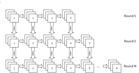
This practically enables the ensemble algorithm to train the subsequent rounds for a considerably smaller number of epochs, consequently reducing the overall training time by a large factor. The original paper also provides a conjecture-based justification for why it makes sense to extend the previously trained network to learn the “corrections” taught by the boosting algorithm. A high level description of the method is shown in Algorithm 5, and the structure of the network at each round is illustrated in Figure 3.

Algorithm 5 Deep Incremental Boosting

Inputs: training setX0, a modifiable algorithm to create classifier hypothesesh(X)

D0,i= 1/M for alli

t= 0

whilet < tend do

ut←create untrained classifier with additional layer of shapeLnew copy weights fromWt into the bottom layers ofut

ht←trainut classifier on current subset

Wt+1←all weights fromht

t= 1₂P(i,y)∈BDt,i(1−ht(xi, yi) +ht(xi, y))

βt=t/(1−t)

Dt+1,i=

Dt,i

Zt ·β

(1/2)(1+ht(xi,yi)−ht(xi,y))_|∀_i_{= 1}_{· |}_x_|

αt=_β1

t

t=t+ 1

end while

H(x) = argmaxy∈Y

PT

(11)

X

Fig. 3: Example illustration of how new members of the ensemble are created in each subsequent round of Deep Incremental Boosting. At each round a new layer is added to the previous network, starting atp0 = 4. The weights of all layers

below the newly inserted one are copied between rounds.

5 Creating the Boosted Residual Network

In this section we propose a method for generating Boosted Residual Networks. This works by increasing the size of an original residual network by one resid-ual block at each round of boosting. The method achieves this by selecting an

injection point indexpiat which the new block is to be added. It is to be noted

that pi is not necessarily the last block in the network.

The boosting method performs an iterative re-weighting of the training set, which skews the resample at each round toemphasizethe training examples that are harder to learn. Therefore, it becomes necessary to utilise the entire ensemble at test time, rather than just use the network trained in the last round. It is also possible to delete individual blocks from a Residual Network at training and/or testing time, as presented in [15], however this issue is considered out of the scope of this paper.

The iterative algorithm used in the paper is shown in Algorithm 6. At the first round, the entire training set is used to train a network of the originalbase

architecture, for a number of epochsn0. After the first round, the following steps

are taken at each subsequent roundt:

– The ensemble constructed so far is evaluated on the training set to obtain the set errors, so that a new training set can be sampled from the original training set. This is a step common to all boosting algorithms.

– A new network is created with the same structure as that of the previous round. To this network, a new block of layersBnew is added immediately

after positionpt, which is determined as an initial pre-determined position

p0plus an offsetP_i=1_→_pδifor all the blocks added at previous layers, where

(12)

XI

the new block of layers immediately after the block of layers added at the previous round, so that all new blocks are effectively added sequentially.

Bnewis not a residual block, but usally consists of a group of different layers

(e.g. batch normalization, convolution, and activation).

– The weights from the layers belowpt are copied from the network trained

at roundt−1 to the new network. This step allows to considerably shorten the training thanks to the transfer of learning shown in [46].

– The newly created network is subsequently trained for a reduced number of epochsnt.

– The new network is added to the ensemble following the conventional rules and weightαt=_β1

t used in AdaBoost. We did not see a need to modify the

wayβtis calculated, as it has been performing well in both DIB and many

AdaBoost variants [34,35,9,23].

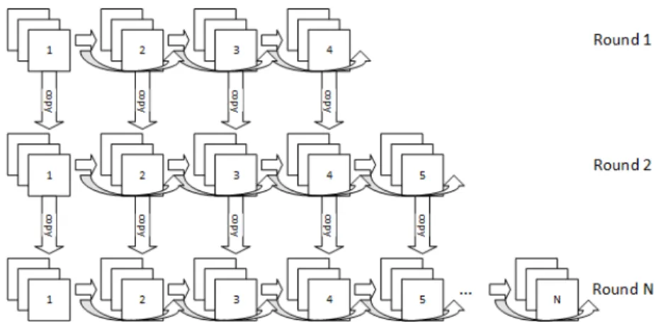
Figure 4 shows a diagram of how the Ensemble is constructed by deriving the next network at each round of boosting from the network used in the previous round.

Fig. 4: Illusration of subsequent rounds of Boosted Residual Networks

We identified a number of optional variations to the algorithm that may be implemented in practice, which we have empirically established as not having a significant impact on the overall performance of the network. We report them here for completeness.

– Freezing the layers that have been copied from the previous round and per-form a round of “local learning” by only training the new layers, before performing an (optional) round of “global learning”. This is common prac-tice for many supervised and unsupervised transfer learning approaches and could provide a valuable improvement in performance for some datasets.

(13)

XII

Algorithm 6 Boosted Residual Networks

Inputs: training setX0, a modifiable algorithm to train Residual Network hypotheses

h(X)

D0,i= 1/M for alli

t= 0

p0←initial injection position

whilet < T do

ut←create untrained classifier with an additional blockBnew of pre-determined shapeNnew

determine block injection positionpt=pt−1+|Bnew| connect the input ofBnew to the output of layerpt−1

connect the output ofBnew and of layerpt−1 to a merge layermi connect the merge layer to the remainder of the network

copy weights fromWt into the bottom layersl < pt ofut

Wt+1←all weights fromht

t=Pi:ht(xi)6=yiDt(i)

if t>1₂ then abort loop

end if

βt=t/(1−t)

Dt+1,i=

Dt,i

Zt ·

(

βt if ht(xi) =yi

1 otherwise |∀i= 1· |x|

αt=_β1

t

t=t+ 1

end while

H(x) = argmax_y∈Y

PT

(14)

XIII

– Inserting the new block always at the same position, rather than after the previously-inserted block (we found this to affect performance negatively).

In the extreme cases where the base classifier learns the training set very well (or indeed perfectly), the value of αt goes towards its asymptote of + inf.

This causes problems with both resampling weights and ensemble weights, so it is necessary to cap the value of αt. Empirically, bounds of (10−3,103) have

proven to contain the runaway effects whilst not affecting the learning in the non–degenerate case.

In a similar way to how SAMME.R extends SAMME, we present BRN.R as an extension of BRN, which derives its boosting procedure from SAMME.R to take advantage of the samereal-valued classifiers. BRN.R is shown in Algo-rithm 7.

Algorithm 7 BRN.R

Inputs: training setX0, a modifiable algorithm to create classifier hypothesesh(X)

D0,i= 1/M for alli

t= 0

whilet < tend do

Obtain weighted class probability estimatespi(X) =Pt(y=ci|Xt, ht), i= 1. . . k

replaceht(Xt)←(K−1)

logpi(X)−1

k

Pk

j=1logpj(X)

, i= 1. . . k

Dt+1,i=

Dt,i

Zt e

−k−1

k y

T_log_p(X

ta₎_|∀_i_{= 1}_{· |}_x_|

t=t+ 1

end while

H(x) = argmaxy∈Y

PT

t=1ht(x, y)

5.1 The sensitivity of additional hyperparameters

(15)

XIV

First, we consider the position pt at which a new residual block Bnew is

injected into the network. This governs the structure of the network at each boosting round, but more importantly, the number of layers that will have their weights initialised from a copy of the previous round. In our experiments we found that using the maximum possible value ofptat each round produced the

best results, both in generalisation ability and training speed up - we were able to reduce the number of training epochs for the subsequent rounds (t >1) by a greater amount when the value ofpt was higher. Intuitively, this indicates that

transferring a higher number of layers produces higher benefits.

Second, we consider the fact that a cut-off pointtmax could be introduced

for no longer adding new residual blocks. Our experiments indicated that, for ten rounds of boosting, adding such a cut-off point did not produce any further improvements. However, when generating much larger ensembles (for example 1000 members) it will likely be beneficial to provide an upper limit to the size of the networks being produced. Even though there have been residual networks with over 1000 layers[47,15], it has not been guaranteed that adding and in-definite number of residual blocks will always produce better results. Adding this constraint will also help contain the amount of computation required and therefore the speed of training each member.

Third, the structure of the new residual blockBnewhas to be chosen

appro-priately. In residual networks, each block tends to belong to one of a fewfamilies

of blocks defined in the structure of each network. Our experiments confirm that the best strategy is to create the new blockBnew such that its structure is the

same as its predecessor block Bpt. This results in each boosting round creating

a “longer” version of the original network, without the addition of new families of blocks.

6 A related approach based on Bagging

Bagging (short for “bootstrap aggregating”) is a technique that is based on the statistical bootstrapping method, originally introduced in [5], where the original author also shows a number of applied use cases. A quantityN of bootstraps is created by randomly pickingM elements from a training dataset of sizeZ with re-sampling, and then using each of these bootstraps to train a separate identical base classifier. Ref [5] introduces Bagging withM =Z, and this practice seems to be observed in most of the literature. This will create diverse members because of the randomized re-sampling, but because there will be significant overlap in the training sets, all the members will still have positive correlation.

(16)

XV

The principle of additively creating an ensemble of progressively larger resid-ual networks, when extended to bagging, generates a less complex process. We call this the Bagged Residual Network (BaRN). This method offers the same advantages and disadvantages that Bagging offers over boosting. Based on the original Bagging recipe [5], the algorithm is illustrated in Algorithm 8.

Algorithm 8 Bagged Residual Networks

t= 0

p0←initial injection position

whilet < T do

Xt←sample fromX0 with uniform distribution

t=t+ 1

end while

H(x) = argmax_y∈Y

PT

t=1logαtht(x, y)

7 Distilled Ensembles

It has been shown [3] that it is possible to approximate a deep neural network by using a more shallow one that is subsequently trained on its output, with the goal to emulate its output function. No restriction is mentioned with regards to generalizing this approach to Ensembles, and it should be theoretically possible to train a smaller model to perform like the larger one, as has been done, for example, in [6], where the authors have developed a new set of algorithms to approximate larger Ensembles.

The process of distillation, introduced in Ref [18], produces small networks that emulate the behaviour of larger, more complex ones. It does so by utilising the output functionf0₍_X_{) of the}_cumbersome_{model as the target of the learning}

(17)

XVI

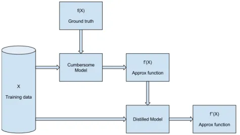
This distillation process has been applied to both BRN, DIB, and BaRN, as it is possible to apply the same principle to all the ensemble learning algorithms. Figure 5 illustrates graphically the distillation process.

Fig. 5: Illustration of the distillation process: the cumbersome model creates an approximate function f0(x) by learning from the training data and the ground truth functionf(x), while the distilled model learns a new second-order approx-imate functionf00(x) from the cumbersome’s approximate function.

8 Experiments and Discussion

ResNet Bagging AdaBoost DIB BRN BRN.R BaRN MNIST 99.41 % 99.46 % 99.42 % 99.47 % 99.53 %99.55%99.55

CIFAR-10 89.12 % 90.43 % 89.74 % 90.83 % 90.85 %91.04% 90.82 CIFAR-10 (aug) 92.14 % 92.61 % 92.47 % 92.51 % 92.94 %92.96% 92.80 CIFAR-100 67.25 % 68.15 % 69.11 % 69.16 % 70.79 %71.94% 69.42 CIFAR-100 (aug) 69.72 % 71.90 % 69.82 % 71.60 % 72.41 %73.52% 72.01 TinyImagenet 30.73 % 40.53 % 39.70 % 44.91 % 44.34 %45.68% 42.31

Table 1: Mean test accuracy in the benchmark datasets for the methods com-pared. The best result is highlighted in bold.

(18)

XVII

number of improvements number of speed-ups

MNIST 9 10

CIFAR-10 8 10

CIFAR-10 (aug) 9 10

CIFAR-100 10 3

CIFAR-100 (aug) 10 10

TinyImagenet 10 4

Table 2: The frequency of experimental runs where BRN has the best perfor-mance of all methods examined, both in generalisation and training time.

methods in the literature. A comprehensive list of experiments in the litera-ture that have used these benchmarks can be found in Ref [12]. We compared Boosted Residual Networks (BRN) with an equivalent Deep Incremental Boost-ing without the skip-connections (DIB), AdaBoost and BaggBoost-ing with both the initial network as the base classifier (AdaBoost) and the single Residual Net-work equivalent to the last round of Boosted Residual NetNet-works (ResNet), and Bagged Residual Networks (BaRN). All the parameters for training have been kept fixed for all experiments and no further hyperparameter optimisation has been done on the base classifiers beyond that for improving the performance of the individual network (ResNet). We performed a manual hyperparameter search for the individual residual network, before running the first experiment, on a small subset of each dataset, using 10000 images for training and 10000 for testing. We then fixed the hyperparameters we found, and used them for every experiment we ran for the dataset in question.

In order to reduce noise in the results, we aligned the random initialisation of all network weights across experiments, by fixing the seeds for the random number generators. All experiments were repeated 10 times and we report the mean accuracy values. This approach has guaranteed control over the variables that could have affected the learning, leaving only the ensemble method and its specific hyperparameters as the free variables being evaluated.

As already mentioned, MNIST [21] is a common computer vision dataset that associates 70000 pre-processed images of hand-written numerical digits with a class label representing that digit. The input features are the raw pixel values for the 28×28 images, in grayscale, and the outputs are the numerical value between 0 and 9. 50000 samples are used for training, 10000 for validation, and 10000 for testing.

CIFAR-10 is a dataset that contains 60000 small images of 10 categories of objects. It was first introduced in [20]. The images are 32×32 pixels, in RGB format. The output categories are airplane, automobile, bird, cat, deer, dog,

frog, horse, ship, truck. The classes are completely mutually exclusive so that it

(19)

XVIII

CIFAR-100 is a dataset that contains 60000 small images of 100 categories of objects, grouped in 20 super-classes. It was first introduced in [20]. The image format is the same as CIFAR-10. Class labels are provided for the 100 classes as well as the 20 super-classes. A super-class is a category that includes 5 of the fine-grained class labels (e.g. “insects” containsbee, beetle, butterfly, caterpillar,

cockroach). 50000 samples are used for training, and 10000 for testing. This

dataset was originally constructed without a validation set.

TinyImagenet is a simplified version of the Imagenet challenge dataset [33]. It has 120000 images, split into 100000 for training, 10000 for validation and 10000 for testing, each 64×64 pixels in size. The dataset comprises of 200 different classes, equally balanced through each split of the dataset. It is derived completely from a small sample of the original Imagenet dataset. Because the labels for the test set have not been released to the public, for this dataset we had to use the validation set as the test set.

(20)

XIX

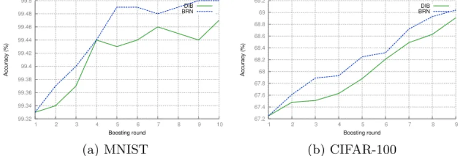
the errors this represents an error reduction from 0.53% to 0.45%, which reflects a mean relative error reduction of 15%. Figure 6 shows a side-by-side compari-son of accuracy levels at each round of boosting for both DIB and BRN on the MNIST and CIFAR-100 test sets. This figure illustrates how BRNs are able to consistently outperform DIB at each intermediate value of ensemble size, and although such differences would still fall within a Bernoulli confidence interval of 95%, we make the note that this does not take account of the fact that all the random initialisations were aligned, so both methods started with the exact same network. In fact, an additional Friedman Aligned Ranks test on the entire group of algorithms tested shows that there is a statistically significant differ-ence in generalisation performance, whilst a direct Wilcoxon test with a null hypothesis that BRN and DIB are sampled from the same distribution shows that BRN is significantly better. In both cases, the “sample” is the average of all experiments with the same characteristics (dataset and method), rather than the single experiment run. This is also corroborated by the “number of wins” on each dataset (Table 2), and the “number of datasets won” by BRN vs the other methods (Table 1).

99.32 99.34 99.36 99.38 99.4 99.42 99.44 99.46 99.48 99.5

1 2 3 4 5 6 7 8 9 10

Accuracy (%) Boosting round DIB BRN (a) MNIST 67.2 67.4 67.6 67.8 68 68.2 68.4 68.6 68.8 69 69.2

1 2 3 4 5 6 7 8 9

Accuracy (%)

Boosting round DIB BRN

(b) CIFAR-100

Fig. 6: Round-by-round comparison of DIB vs BRN on the test set

Figure 7 shows how BRN.R generally achieves better performance at almost every boosting round. This may be partly because BRN.R is tailored more to-wards the type of datasets used as benchmarks – the use of the continuous probability output from the CNNs is a big factor.

Table 3 shows that this is achieved without significant changes in the training time1_{. The main speed increase is due to the fact that the only network being}

trained with a full schedule is the first network, which is also the smallest, whilst all other derived networks are trained for a much shorter schedule (in this case only 10% of the original training schedule). If we exclude the single network,

1 _{In a few cases BRN is actually faster than DIB, but we believe this to be just}

(21)

XX 89 89.2 89.4 89.6 89.8 90 90.2 90.4 90.6 90.8 91 91.2

1 2 3 4 5 6 7 8 9 10

Accuracy (%) Boosting round BRN BRN.R (a) CIFAR-10 67.5 68 68.5 69 69.5 70 70.5 71 71.5 72

1 2 3 4 5 6 7 8 9 10

Accuracy (%)

Boosting round

BRN BRN.R

(b) CIFAR-100

Fig. 7: Round-by-round comparison of BRN vs BRN.R on the test set

which is clearly from a different distribution and only mentioned for reference, a Friedman Aligned Ranks test [10] shows that there is a statistically significant difference in speed between the members of the group, but, as can be expected, a Wilcoxon test [45] between Deep Incremental Boosting and Boosted Residual Networks does not show a significant difference. This confirms what could be conjured from the algorithm itself for BRN, which is of the same complexity w.r.t. the number of Ensemble members as DIB. The confirmation that the con-sistency of improvements is significant, combined with the fact that the method is significantly faster than training the equivalent network from the final round for the full number of epochs, presents an effective strategy for improving per-formance without requiring additional resources and in less time. The specific time improvement is highly dependent on the number of epochs chosen for the subsequent training rounds et,∀t > 0, and the number of boosting rounds t,

however we find empirically that choosing a set of such parameters that keep the total training time low is feasible.

The hardware used to train each network was identical for every case, and because in all cases the ensemble members were trained sequentially, ours was the only work running on the system, providing a sufficiently controlled environment to justify using wall-clock time as a measurement of speed. Table 2 shows that BRN is the fastest method most of the time, whilst Table 3 shows the magnitude of the time improvements, which indicate that the speed improvement on regular ensemble methods is noteworthy and consistent.

(22)

XXI

to reach state-of-the-art on these datasets are very cumbersome in terms of resources and training time [15]. Instead, we used relatively simpler network ar-chitectures that were faster to train while still performing well on the datasets at hand, with accuracy close to and almost comparable to the state-of-the-art. This enabled us to test larger Ensembles within an acceptable training time. Our intention is to demonstrate a methodology that makes it feasible to create ensembles of Residual Networks following acustomised approach to significantly improve the training times and accuracy levels achievable with current ensemble methods.

ResNet Base Net Bagging AdaBoost DIB BRN BRN.R BaRN

MNIST 217 62 437 442 202 199 207 209

CIFAR-10 1941 184 1193 1212 461 449 453 458 CIFAR-10 (aug) 2228 213 2138 2150 1031 911 943 955 CIFAR-100 2172 303 2762 2873 607 648 659 676 CIFAR-100 (aug) 2421 328 3044 3072 751 735 742 764 TinyImagenet 4804 619 6031 6288 15911613 1716 1645

Table 3: Training times comparison, in minutes. BRN and DIB are the fastest Ensemble methods compared. The time to train the individual base network and a ResNet of comparable performance is reported for comparison.

Training used the WAME method ([26]), which has been shown to be faster than Adam and RMSprop, whilst still achieving comparable generalisation. This is thanks to a specific weight-wise learning rate acceleration factor that is de-termined based only on the sign of the current and previous partial derivative

∂E(x)

∂wij . For the single Residual Network, and for the networks in AdaBoost, we

trained each member for 100 epochs. For Deep Incremental Boosting and all variants of Boosted Residual Networks, we trained the first round for 50 epochs, and every subsequent round for 10 epochs, and ran all the algorithms for 10 rounds of boosting (except for the single network). We chose to use less epochs for the first round because we found empirically that the additional epochs that fine-tuned the base network were not improving the performance at subsequent rounds in any significant way. Because our intention was to find an ensemble method that would train in significantly less time without loss of generalisation, we found that this was an effective strategy. Similarly, we found that above 10 rounds the time to train the ensemble was increasing without large improvements to generalisation.

The structure of the base network at the first round is shown in Table 5. This was created by taking the shape (strides, number of convolutions) of existing blocks of ResNet-50, and making the network smaller to create a reasonable starting point that still performed well.

(23)

XXII

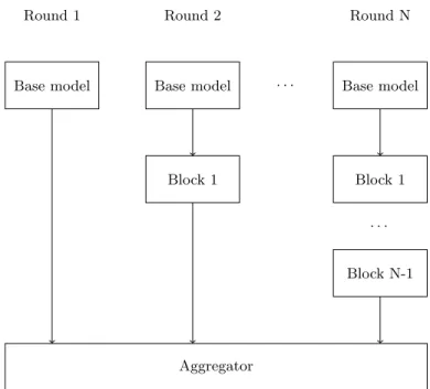
and in Table 6b for CIFAR-10, CIFAR-100 and TinyImagenet. The architecture of the ensemble at the Nth_{round of boosting is shown in Figure 8.}

learning rate epochs batch size

MNIST 10−2 ₁₀₀ ₆₄

CIFAR-10 10−3, 10−4after 40 epochs 100 128 CIFAR-10 (aug) 10−3_{, 10}−4_{after 40 epochs} ₁₀₀ ₁₂₈

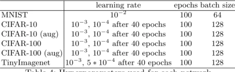
CIFAR-100 10−3, 10−4after 40 epochs 100 128 CIFAR-100 (aug) 10−3, 10−4after 40 epochs 100 128 TinyImagenet 10−3_{, 5}_∗₁₀−4_{after 40 epochs} ₁₀₀ ₁₂₈

Table 4: Hyperparameters used for each network

The choice of additional block was based on the typical structure of a block in residual networks: Convolution, followed by Batch Normalization, followed by Rectified Linear Units activation. For convenience, we chose to use the same number of filters, shape, and stride as the convolutional layers that each block succeeds. All layers were initialised following the recommendations in [16]. Any additional network hyperparameters are reported in Table 4.

An additional experiment on TinyImagenet with BRN.R and 20 epochs at each round (instead of 10), has an even higher test accuracy of 46.78%, showing that it is possible to fine-tune the number of subsequent epochs as a hyperpa-rameter to obtain better results. We only report this result for completeness and it was not included in any statistical test.

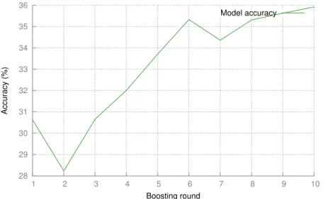
Observing unrolled iterative estimation in BRN Especially for the more complex datasets such as CIFAR-100 and TinyImagenet, the accuracy of the individual classifier improves considerably at each round. We attribute most of this to the fact that, by focusing the training on the newly added block, we are explicitly encouraging the layer-by-layer refinements discussed in the treaty of Unrolled Iterative Estimation [13]. Figure 9 shows the observed accuracy on TinyImagenet at each round.

(24)

XXIII

Round 1

Base model

Round 2

Base model

Block 1

. . .

Round N

Base model

Block 1

Block N-1

. . .

Aggregator

(25)

XXIV

28 29 30 31 32 33 34 35 36

1 2 3 4 5 6 7 8 9 10

Accuracy (%)

Boosting round

Model accuracy

Fig. 9: Single-model test accuracy for each round of BRN on TinyImagenet

Despite the fact that BRN has better performance, the benefits of using BaRN are:

– The reduction of sensitivity to highly imbalance datasets, a known issue for boosting algorithms

– The potential to derive parallel and distributed implementations which ap-proximate the final ensemble

– The use of dynamic distortions and transformations of the original data

8.1 Additional experiments with distillation

In another set of experiments we tested the performance of a Distilled Boosted Residual Network (DBRN) and a Distilled Bagged Residual Network (DBaRN). For the structure of the final distilled network we used the same architecture as that of the Residual Network from the final round of boosting. Average accuracy results in testing over 10 runs are presented in Table 7, and for completeness of comparison we also report the results for the distillation of DIB, following the same procedure, as DDIB. DBRN does appear to improve results only for CIFAR-10, but it consistently beats DDIB on all datasets. These differences are too small to be deemed statistically significant with a Friedman Aligned ranks test, confirming the hypothesis that the functions are sampled from the same distribution. It can therefore be said that the function learned by both BRN and DIB can be efficiently transferred to a single network, for the datasets taken under consideration.

(26)

XXV

cannot simply replace the distillation process by utilising the network created in the last round of BaRN. This also refutes our hypothesis that BaRN could be used as a method for incrementally creating a large residual network.

64 conv, 5×5 2×2 max-pooling

128 conv, 5×5 2×2 max-pooling *

64 conv, 3×3 Dense, 1024 nodes

50% dropout

(a) MNIST

2×96 conv, 3×3 96 conv, 3×3, 2×2 strides 96 conv, 3×3, 2×2 strides 96 conv, 3×3, 2×2 strides

2×2 max-pooling 2×192 conv, 3×3 192 conv, 3×3, 2×2 strides 192 conv, 3×3, 2×2 strides 192 conv, 3×3, 2×2 strides

2×2 max-pooling 192 conv, 4×3 192 conv, 3×3 *

192 conv, 3×3 192 conv, 1×1 10 conv, 1×1 global average pooling

10-way softmax2

(b) CIFAR-10, CIFAR-10, and TinyImagenet

Table 5: Initial Network structures used in experiments. The layers marked with “*” indicate the location after which we added the new residual blocks at each round of DIB and BRN. Batch normalisation and activation layers are omitted from this diagram for simplicity.

9 Conclusions and future work

In this paper we introduced a customised methodology for creating ensembles of deep learning models, and design three algorithms that follow this approach, specifically tailored to Convolutional Networks to generate Boosted Residual Networks and Bagged Residual Networks, and looked at potential variants of those algorithms for real-valued classifiers. We have shown that this surpasses the performance of a single Residual Network equivalent to the one trained at the last round of boosting, of an ensemble of such networks trained with AdaBoost, and of the equivalent Deep Incremental Boosting on the MNIST, CIFAR-10, CIFAR-100, and TinyImagenet datasets, with and without using common data augmentation techniques.

2

(27)

XXVI

64 conv, 3×3 Batch Normalization

ReLu activation

(a) MNIST

192 conv, 4×3 Batch Normalization

ReLu activation 192 conv, 3×3 Batch Normalization

ReLu activation

(b) 10, CIFAR-100, and TinyImagenet

Table 6: Structure of blocks added at each round of DIB and BRN.

DBRN DBRN.R DDIB DBaRN BaRN-l MNIST 99.49 % 99.50 % 99.44 % 99.55 % 99.35 % CIFAR-10 91.11 % 91.05 % 90.66 % 90.77 % 90.62 % CIFAR-10 (aug) 93.28 % 92.76 % 92.43 % 92.68 % 92.73 % CIFAR-100 68.99 % 68.86 % 65.91 % 67.42 % 66.16 % CIFAR-100 (aug) 70.24 % 70.71 % 69.18 % 71.51 % 70.44 % TinyImagenet 42.63 % 43.70 % 42.14 % 39.64 % 32.92 %

Table 7: Testing accuracy for distilled variants of the ensembles.

We then derived and looked at distilled versions of the methods, and how this technique can serve as an effective way to reduce the test-time cost of running the Ensemble. We analysed how this compares to the distilled version of the same baselines used in the preceding experiment.

The combination of such techniques has shown that it is possible to train a model that has slightly better generalisation with lower complexity in a signifi-cantly shorter amount of time.

Because of the limitations to the network size imposed in our experiments, it might be appealing in the future to evaluate the performance improvements obtained when creating ensembles of large, state-of-the-art, base networks, for example by using the 1001-layer networks found in [15] as a starting network architecture.

(28)

signifi-XXVII

cant. We believe it is however still necessary to further investigate this approach and the behaviour of additive training in isolation.

Additional further investigation could also be conducted on the creation of Boosted Densely Connected Convolutional Networks, by applying the same prin-ciple to DCCN instead of Residual Networks.

Another very important property that has not been fully explored in this paper is the recent development of Attack and Defense methods for adversarial training using Ensembles [40]. Whilst we do not investigate the effect of cus-tomised ensemble methods on adversarial learning, it is possible to speculate that, either with or without adaptations to the learning setup, these methods could be used to improve on such a class of problems.

We also believe that there is additional work in exploring how such itera-tive methods like BRN may be extended to incorporate notions of differential computation in deep learning, such as LM-ResNet and LM-ResNeXt [2], and NAIS-Net [1].

10 Conflict of interests

The authors have received a hardware grant from NVIDIA for this research.

References

1. Ciccone, M., Gallieri, M., Masci, J., Osendorfer, C., Gomez, F.: NAIS-Net: Stable Deep Networks from Non-Autonomous Differential Equations. CoRR abs/1804.07209 (2018),http://arxiv.org/abs/1804.07209

2. Lu, Y., Zhong, A., Li, Q., Dong, B.: Beyond Finite Layer Neural Networks: Bridging Deep Architectures and Numerical Differential Equations. ICLR (2018), https: //openreview.net/forum?id=ryZ283gAZ

3. Ba, L.J., Caurana, R.: Do deep nets really need to be deep? Advances in neural information processing systems pp. 2654–2662 (2014)

4. Bishop, C.: Neural Networks for Pattern Recognition. Oxford University Press (1995)

5. Breiman, L.: Bagging predictors. Machine Learning 24(2), 123–140 (1996) 6. Bucilu, C., Caruana, R., Niculescu-Mizil, A.: Model compression. In: Proceedings

of the 12th ACM SIGKDD international conference on Knowledge discovery and data mining. pp. 535–541. ACM (2006)

7. Clevert, D., Unterthiner, T., Hochreiter, S.: Fast and accurate deep network learning by exponential linear units (elus). CoRR abs/1511.07289 (2015), http: //arxiv.org/abs/1511.07289

8. Dietterich, T.G.: An experimental comparison of three methods for constructing ensembles of decision trees: Bagging, boosting, and randomization. Machine learn-ing 40(2), 139–157 (2000)

9. Freund, Y., Iyer, R., Schapire, R.E., Singer, Y.: An efficient boosting algorithm for combining preferences. The Journal of machine learning research 4, 933–969 (2003)

(29)

XXVIII

11. Graham, B.: Fractional max-pooling. CoRR abs/1412.6071 (2014),http://arxiv. org/abs/1412.6071

12. Benenson, R.: What is the class of this image?http://rodrigob.github.io/are_ we_there_yet/build/classification_datasets_results.html

13. Greff, K., Srivastava, R.K., Schmidhuber, J.: Highway and residual networks learn unrolled iterative estimation. arXiv preprint arXiv:1612.07771 (2016)

14. Hastie, T., Rosset, S., Zhu, J., Zou, H.: Multi-class adaboost. Statistics and its Interface 2(3), 349–360 (2009)

15. He, K., Zhang, X., Ren, S., Sun, J.: Deep residual learning for image recognition. arXiv preprint arXiv:1512.03385 (2015)

16. He, K., Zhang, X., Ren, S., Sun, J.: Delving deep into rectifiers: Surpassing human-level performance on imagenet classification. In: Proceedings of the IEEE Interna-tional Conference on Computer Vision. pp. 1026–1034 (2015)

17. He, K., Zhang, X., Ren, S., Sun, J.: Identity mappings in deep residual networks. arXiv preprint arXiv:1603.05027 (2016)

18. Hinton, G., Vinyals, O., Dean, J.: Distilling the knowledge in a neural network. arXiv preprint arXiv:1503.02531 (2015)

19. Huang, G., Liu, Z., Weinberger, K.Q.: Densely connected convolutional networks. arXiv preprint arXiv:1608.06993 (2016)

20. Krizhevsky, A., Hinton, G.: Learning multiple layers of features from tiny images (2009)

21. Lecun, Y., Cortes, C.: The MNIST database of handwritten digitshttp://yann. lecun.com/exdb/mnist/

22. Malakooti, B., Zhou, Y.Q.: Feedforward artificial neural networks for solving dis-crete multiple criteria decision making problems. Management Science 40(11), 1542–1561 (1994)

23. Mosca, A., Magoulas, G.: Deep incremental boosting. In: Benzmuller, C., Sutcliffe, G., Rojas, R. (eds.) GCAI 2016. 2nd Global Conference on Artificial Intelligence. EPiC Series in Computing, vol. 41, pp. 293–302. EasyChair (2016)

24. Mosca, A., Magoulas, G.: Boosted Residual Networks. In: EANN 2017. 18th Inter-nationa Conference on Engineering Applications of Neural Networks.

25. Mosca, A., Magoulas, G.D.: Regularizing deep learning ensembles by distillation. In: 6th International Workshop on Combinations of Intelligent Methods and Ap-plications (CIMA 2016). p. 53 (2016)

26. Mosca, A., Magoulas, G.D.: Training convolutional networks with weight-wise adaptive learning rates. In: ESANN 2017 proceedings, European Symposium on Ar-tificial Neural Networks, Computational Intelligence and Machine Learning. Bruges (Belgium), 26-28 April 2017, i6doc.com publ. (2017)

27. Mosca, A., Magoulas, G.D.: Distillation of deep learning ensembles as a regulari-sation method. In: Advances in Hybridization of Intelligent Methods, pp. 97–118. Springer (2018)

28. Mukherjee, I., Schapire, R.E.: A theory of multiclass boosting. Journal of Machine Learning Research 14(Feb), 437–497 (2013)

29. Oquab, M., Bottou, L., Laptev, I., Sivic, J.: Learning and transferring mid-level image representations using convolutional neural networks. In: Proceedings of the IEEE conference on computer vision and pattern recognition. pp. 1717–1724 (2014) 30. P laczek, S., Adhikari, B.: Analysis of multilayer neural networks with direct and

cross forward connection. Fundamenta Informaticae 133(2-3), 227–240 (2014) 31. Raiko, T., Valpola, H., LeCun, Y.: Deep learning made easier by linear

(30)

XXIX

32. Ripley, B.D.: Pattern recognition and neural networks. Cambridge university press (2007)

33. Russakovsky, O., Deng, J., Su, H., Krause, J., Satheesh, S., Ma, S., Huang, Z., Karpathy, A., Khosla, A., Bernstein, M., Berg, A.C., Fei-Fei, L.: ImageNet Large Scale Visual Recognition Challenge. International Journal of Computer Vision (IJCV) 115(3), 211–252 (2015)

34. Schapire, R.E.: The strength of weak learnability. Machine Learning 5, 197–227 (1990)

35. Schapire, R.E., Freund, Y.: Experiments with a new boosting algorithm. Machine Learning: proceedings of the Thirteenth International Conference pp. 148–156 (1996)

36. Schraudolph, N.: Accelerated gradient descent by factor-centering decomposition (1998)

37. Schraudolph, N.N.: Centering neural network gradient factors. In: Neural Net-works: Tricks of the Trade, pp. 205–223. Springer (2012)

38. Srivastava, R.K., Greff, K., Schmidhuber, J.: Training very deep networks. In: Advances in neural information processing systems. pp. 2377–2385 (2015) 39. Srivastava, R.K., Greff, K., Schmidhuber, J.: Highway networks. arXiv preprint

arXiv:1505.00387 (2015)

40. Tram`er, F., Kurakin, A., Papernot, N., Goodfellow, I., Boneh, D., Mc-Daniel, P.: Ensemble adversarial training: Attacks and defenses. arXiv preprint arXiv:1705.07204 (2017)

41. Vatanen, T., Raiko, T., Valpola, H., LeCun, Y.: Pushing stochastic gradient to-wards second-order methods–backpropagation learning with transformations in nonlinearities. In: International Conference on Neural Information Processing. pp. 442–449. Springer (2013)

42. Veit, A., Wilber, M., Belongie, S.: Residual Networks Behave Like Ensembles of Relatively Shallow Networks. ArXiv e-prints (May 2016)

43. Wan, L., Zeiler, M., Zhang, S., Cun, Y.L., Fergus, R.: Regularization of neural networks using dropconnect. In: Proceedings of the 30th International Conference on Machine Learning (ICML-13). pp. 1058–1066 (2013)

44. Whitley, D., Starkweather, T., Bogart, C.: Genetic algorithms and neural networks: Optimizing connections and connectivity. Parallel computing 14(3), 347–361 (1990) 45. Wilcoxon, F.: Individual comparisons by ranking methods. Biometrics 1(6), 80–83

(1945)

46. Yosinski, J., Clune, J., Bengio, Y., Lipson, H.: How transferable are features in deep neural networks? In: Advances in Neural Information Processing Systems. pp. 3320–3328 (2014)