Missing a trick: Karatsuba variations
Michael Scott
MIRACL Labs
Abstract. There are a variety of ways of applying the Karatsuba idea to multi-digit multiplication. These apply particularly well in the context where digits do not use the full word-length of the computer, so that partial products can be safely accumulated without fear of overflow. Here we re-visit the “arbitrary degree” version of Karatsuba and show that the cost of this little-known variant has been over-estimated in the past. We also attempt to definitively answer the question as to the cross-over point where Karatsuba performs better than the classic method.
1
Introduction
As is well known the Karatsuba idea for calculating the product of two poly-nomials can be used recursively to significantly reduce the number of partial products required in a long multiplication calculation, at the cost of increas-ing the number of additions. A one-level application can save 1/4 of the partial products, and a two-level application can save 7/16ths etc. However application of Karatsuba in this way is quite awkward, it attracts a large overhead of extra additions, and the ideal recursion is only available if the number of digits is an exact power of two.
One way to make Karatsuba more competitive is to use a number base radix that is somewhat less than the full register size, so that additions can be accu-mulated without overflow, and without requiring immediate carry propagation. Here we refer to this as a “reduced-radix” representation.
Multi-precision numbers are represented as an array of computer words, or “limbs”, each limb representing a digit of the number. Each computer word is typically the same size as the processor’s registers, that are manipulated by its instruction set. Using a full computer word for each digit, or a “packed-radix” representation [7], intuitively seems to be optimal, and was the method originally adopted by most multi-precision libraries. However to be efficient this virtually mandates an assembly language implementation to handle the flags that catch the overflows that can arise, for example, from the simple act of adding two digits.
elliptic curve [7]. A reduced-radix representation is sometimes considered to be more efficient [7] – and this is despite the fact that in many cases it will require an increased number of limbs.
In [1] is described an elliptic curve implementation that uses this technique to demonstrate the superiority of using the Karatsuba idea in a context where each curve coordinate is represented in just 16 32-bit limbs. In fact there is much confusion in the literature as to the break-even point where Karatsuba becomes superior. One confounding factor is that whereas Karatsuba trades multiplica-tions for addimultiplica-tions, in modern processors multiplicamultiplica-tions may be almost as fast as additions.
Elliptic curve sizes have traditionally been chosen to be multiples of 128-bits, to provide a nice match to standard levels of security. On the face of it, this is fortuitous, as for example a 256-bit curve might have its x and y coordinates fit snugly inside of 4 64-bit or 8 32-bit computer words using a packed-radix representation. Again, as these are exact powers of 2, they might be thought of as being particularly suitable for the application of the Karatsuba idea. However somewhat counter-intuitively this is not the case – if Karatsuba is to be compet-itive the actual number base must be a few bits less than the word size in order to facilitate addition of elements without carry processing (and to support the ability to distinguish positive and negative numbers). So in fact a competitive implementation would typically require 5 64-bit or 9 32-bit words, where 5 and 9 are not ideal polynomial degrees for the application of traditional Karatsuba. What is less well known is that there is an easy to use “arbitrary degree” variant of Karatsuba (ADK), as it is called by Weimerskirch and Paar [12], which can save nearly 1/2 of the partial products and where the polynomial degree is of no concern to the implementor. In fact this idea has an interesting history. An earlier draft of the Weimerskirch and Paar paper from 2003 is referenced in [10]. But it appears to have been discovered even earlier by Khachatrian et al. [8]1, and independently by David Harvey, as reported in Exercise 1.4 in the textbook [3]. Essentially the same idea was used by Granger and Scott [4], building on earlier work from Granger and Moss [5] and Nogami et al. [11], in the context of a particular form of modular arithmetic.
Here we consider the application of this variant to the problem of long integer multiplication. Since the number of partial products required is the same as the well known squaring algorithm, squaring is not improved, and so is not consid-ered further here. We restrict our attention to the multiplication of two equal sized numbers, as arises when implementing modular arithmetic as required by common cryptographic implementations.
2
The ADK algorithm
This algorithm is described in mathematical terms in [3], [8] and [12]. However here we have used the subtractive variant of Karatsuba to some advantage to get a simpler formula, as pointed out to us by [13].
1
xy=
n−1
∑
i=1
i−1
∑
j=0
(xi−xj)(yj−yi)bi+j+ n∑−1
i=0
bi
n∑−1
j=0
xjyjbj (1)
Observe that in additive form the formula is more
complex:-xy=
n∑−1
i=1
i−1
∑
j=0
(xi+xj)(yi+yj)bi+j+ 2 n∑−1
i=0
xiyib2i− n∑−1
j=0
bj
n∑−1
i=0
xiyibi (2)
This clearly involves more additions and subtractions than equation (1). In fact we find the mathematical description unhelpful in that it makes the method look more complex than it is. It also makes it difficult to determine its exact complexity. To that end an algorithmic description is more helpful.
Algorithm 1The ADK algorithm for long multiplication
Input: Degreen, and radixb= 2t
Input: x= [x0, . . . , xn−1],y= [y0, . . . , yn−1] wherexi, yi∈[0, b−1]
Output: z= [z0, . . . , z2n−2,0], wherezi∈[0, b2−1] andz=xy
1: functionADKmul(x, y)
2: fori←0 ton−1do
3: di ←xiyi
4: end for
5: s←d0
6: z0 ←s
7: fork←1 ton−1do
8: s←s+dk
9: t←s
10: fori←1 +⌊k/2⌋tok do
11: t←t+ (xi−xk−i)(yk−i−yi)
12: end for
13: zk←t
14: end for
15: fork←nto 2n−2do
16: s←s−dk−n
17: t←s
18: fori←1 +⌊k/2⌋ton−1do
19: t←t+ (xi−xk−i)(yk−i−yi)
20: end for
21: zk←t
22: end for
23: returnz
24: end function
propa-gation, which reduces the productzto a radixbrepresentation. A fully unrolled example of the algorithm in action for the casen= 4 is given in the next section.
3
Comparing Karatsuba variants
As an easy introduction consider the product of two 4 digit numbers, z =xy. The School-boy method (SB) requires 16 multiplications (muls) and 9 double precision adds, which is equivalent to 18 single precision adds. In the sequel when comparing calculation costs a “mul” M is a register-sized signed multi-plication resulting in a double register product. An “add” A is the addition (or subtraction) of two registers. We also make the reasonable assumption that while add, shift or masking instructions cost the same on the target processor, an integer multiply instruction may cost more. So the cost of the SB method here is 16M+18A.
z0=x0y0
z1=x1y0+x0y1
z2=x2y0+x1y1+x0y2
z3=x3y0+x2y1+x1y2+x0y3
z4=x3y1+x2y2+x1y3
z5=x3y2+x2y3
z6=x3y3
(3)
A final “propagation” of carries is also required. Assuming that the number base is a simple power of 2, this involves a single precision masking followed by a double precision shift applied to each digit of the result. The carry must then be added to the next digit. If multiplying twondigit numbers the extra cost is equivalent to (10n−7)A adds. Here we will neglect this extra contribution, as it applies independent of the method used for long multiplication.
Using arbitrary-degree Karatsuba (or ADK), the same calculation takes 10 muls and 11 double precision adds and 12 single precision subs. The total cost is 10M+34A. So overall 6 muls are saved at the cost of 16 adds
z0=x0y0
z1= (x1−x0)(y0−y1) + (x0y0+x1y1)
z2= (x2−x0)(y0−y2) + [x0y0+x1y1] +x2y2
z3= (x3−x0)(y0−y3) + (x2−x1)(y1−y2) + [x0y0+x1y1] + [x2y2+x3y3]
z4= (x3−x1)(y1−y3) +x1y1+ [x2y2+x3y3]
z5= (x3−x2)(y2−y3) + (x2y2+x3y3)
z6=x3y3
Here square brackets indicate values already available from the calculation. Hopefully the reader can see the pattern in this example in order to easily ex-trapolate to higher degree multiplications.
It is an interesting exercise to repeat this calculation using one level of “reg-ular” Karatsuba, and simplifying the result. As can be seen in equation 5 the same calculation requires 12 muls, 10 double precision adds and 4 single precision subs, or equivalently 12M+24A, so 4 muls are saved at the cost of 6 adds.
z0=x0y0
z1= (x1y0+x0y1)
z2= (x2−x0)(y0−y2) +x0y0+ (x1y1+x2y2)
z3= [(x2−x0)](y1−y3) + (x3−x1)[(y0−y2)] + [x1y0+x0y1] + [x3y2+x2y3]
z4= [(x3−x1)][(y1−y3)] + [x1y1+x2y2] +x3y3
z5= (x3y2+x2y3)
z6=x3y3
(5)
Observe that only z1, z3 and z5 are calculated differently. Using two levels of Karatsuba (equation 6), requires 9M+38A, so 7 muls are saved at the cost of 20 adds.
z0=x0y0
z1= (x1−x0)(y0−y1) + (x0y0+x1y1)
z2= (x2−x0)(y0−y2) + [x0y0+x1y1] +x2y2
z3= ([x3−x1]−[x2−x0])([y0−y2]−[y1−y3]) + [(x2−x0)(y0−y2)] + [(x3−x1)(y1−y3)]
+ [(x1−x0)(y0−y1)] + [(x3−x2)(y2−y3)] + [x0y0+x1y1] + [x2y2+x3y3]
z4= (x3−x1)(y1−y3) +x1y1+ [x2y2+x3y3]
z5= (x3−x2)(y2−y3) + (x2y2+x3y3)
z6=x3y3
(6)
Now onlyz3is calculated differently from the ADK approach. It is noteworthy that in [1] the authors deployed two levels of standard Karatsuba, and apparently did not consider the ADK method. However since the ADK approach works on a digit-by-digit basis, and thus applies seemlessly independent of the number of digits, it would appear to offer a nice easily applied compromise solution that extracts a big part of the Karatsuba advantage, without causing an explosion in the number of additions.
involving medium sized numbers, as may for example apply in the context of Elliptic Curve Cryptography.
In passing we observe, as also noted in [3], that the ADK method can be used as an amusing alternative algorithm for pencil-and-paper long multiplication. We would not be surprised to learn of its use in the recreational mathematics literature.
4
Numerical stability
Before proceeding we need to address the problem of numerical stability. We start by assuming that both numbers to be multiplied are fully normalized, that is each digit of x is in the range 0 ≤ xi < b. If they are not, they can be
quickly normalized using a fast mask and shift operation (which works even if some of the digits are temporarily negative). For numerical stability of the long multiplication it is important that the sum of double-precision products that form each row of equation 3, do not cause a signed integer overflow. Assume that b= 2t wheret < won a w-bit wordlength computer. Then the product of two such numbers could be as big as 22t−2t+1+ 1. The longest row consists of
nsuch numbers, plus a carry from the previous row. So each row could not be larger than (n+ 1)(22t−2t+1+ 1). Since it must be possible to distinguish the sign of each partial product this must be strictly less than 22w−1.
For the common wordlengths ofw= 32 andw= 64-bits, and for numbers of the sizes relevant to elliptic curve cryptography, we would expectt to be 28 or 29 on a 32-bit computer, and 61 or 62 for a 64-bit computer. Too large and the stability criteria will not be met. Too small and too many words will be required to represent our numbers, with a loss of efficiency.
We would assume that normally the largest radix possible would be used that is compatible with this stability condition. However there may be other factors at play which might dictate a slightly smaller choice fort– for example if reduction were merged with multiplication [4], or if it were regarded as desirable that field elements could be added without normalization prior to multiplication [7].
5
The true cost of ADK multiplication
In [12] the number of multiplications and additions required for the application of the ADK method is calculated, in the context of polynomial arithmetic. There it is worked out that its performance compared to the school-boy method, given a multiplication to addition cost ratio ofr, is such that they are equivalent forr= 3 irrespective of the degree of the polynomials. The rather neat conclusion might be that unless multiplication takes more than 3 times as long as an addition, the method brings no advantage. And for many real-world processors with hardware support for integer multiplication, this may not be the case.
the cost function used for ADK in [12] appears to be incorrect. The true cost in terms of single precision additions is actually only 2n2+ 2n−6 for the ADK method, compared to the 2n2−4n+ 2 required by SB. In [12] the number of additions is calculated as being of the order of 2.5n2. This dramatically changes the balance between the two contenders. Recall that for SB the number of muls is n2, while for the ADK method it is n(n+ 1)/2. An immediate and striking conclusion is that forn≥12 the total number of muls and adds for ADK becomes less than the total required for SB.
Interestingly Khachatrian et al. [8] appear to have got it wrong as well, over-estimating the number of additions required to an even greater extent, as always requiring 50% more additions than the SB method. However these previous over-estimates may be explained by the authors considering only a packed-radix representation.
muls adds
SB n2 2n2−4n+ 2
ADK n(n+ 1)/2 2n2+ 2n−6
Table 1.Complexity
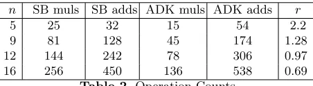
Processor designers go to great lengths to cut the cost in cycles of a mul instruction, even getting it down to 1 clock cycle, the same as that required for an add. However a mul will always require more processor resources, and thus a hidden extra cost will probably show up in actual working code. For example in a multi-scalar architecture only one processor pipeline might support hardware multiplication, whereas all available pipelines will allow simultaneous execution of adds, so whereas one mul can execute in 1 cycle, two or more adds might execute simultaneously. The actual break-even point between ADK and SB can only be determined on a case-by-case basis via an actual implementation. In this next table we calculate the ratiorbetween the costs of muls and adds that mark the expected break-even between SB and ADK.
n SB muls SB adds ADK muls ADK adds r
5 25 32 15 54 2.2
9 81 128 45 174 1.28
12 144 242 78 306 0.97
16 256 450 136 538 0.69
Table 2.Operation Counts
compiler in terms of the number of memory accesses and register move instruc-tions (not considered here) which it might require. However we suspect that any such advantage would be outweighed by the hidden resource consumption of even the fastest integer multiply.
On the other hand it remains a real possibility that a packed-radix imple-mentation of the School-Boy method written in carefully hand-crafted assembly language might prove superior on particular processors, even beyond the 12 limb limit (bearing in mind that a packed-radix representation may actually require less limbs). This could only be established experimentally. A useful resource for comparison purposes would be the well known GMP multi-precision library [6].
6
Some results
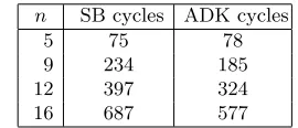
We tested our results on an industry standard Intel i3-4025U 1.9GHz 64-bit processor running in Windows. This is a simple head-to-head comparison of the reduced-radix SB and ADK methods. The test code was written in C, and compiled using the GCC compiler (version 5.1.0) with maximum optimization. It includes the carry propagation code. The multiplication code was fully unrolled, as a compiler cannot always be trusted to do this automatically. Our experience would be that optimized compiler output like this for Intel processors is very hard to improve upon, even using hand-crafted assembly language.
n SB cycles ADK cycles
5 75 78
9 234 185
12 397 324
16 687 577
Table 3.Intel i3-4025U Cycle Counts
These results more than support the conclusion to be drawn from table 2: In fact on this processor the cross-over point occurs already with just 9 limbs. On examining the generated code, it was observed that the number of mul and add-equivalent instructions were as predicted in the analysis above. However an inspection of the generated code also confirmed our suspicion that the ADK code generated more register-register move instructions and memory accesses. On some processors this could offset the ADK advantage.
7
Conclusion
point where Karatsuba variants should be considered ahead of the classic school-boy method for long multiplication.
An obvious extension of the idea applies to Montgomery’s method for mod-ular reduction without division [9] – details are given in an appendix.
Of course we are not claiming that the ADK method is necessarily the best choice in all circumstances. A classic recursive Karatsuba may well be superior in particular cases. For example Hamburg [7] uses a modulus that chimes par-ticularly well with 1-level of classic Karatsuba. And Bernstein et al. [1] may well be correct in applying 2-level Karatsuba in their particular context.
The fact that a multiplication now requires the calculation of the same num-ber of partial products as a squaring, might encourage implementors to use this multiplication algorithm for both squaring and multiplication, so that multipli-cations and squarings cannot be easily distinguished by some simple kinds of side-channel attack, like for example a timing attack.
8
Acknowledgements
References
1. Daniel J. Bernstein, Chitchanok Chuengsatiansup, and Tanja Lange. Curve41417:
Karatsuba revisited. Cryptology ePrint Archive, Report 2014/526, 2014. http:
//eprint.iacr.org/2014/526.
2. Daniel J. Bernstein, Niels Duif, Tanja Lange, Peter Schwabe, and Bo-Yin Yang. High-speed high-security signatures. Cryptology ePrint Archive, Report 2011/368,
2011. http://eprint.iacr.org/2011/368.
3. R. Brent and P. Zimmermann.Modern Computer Arithmetic. Cambridge
Univer-sity Press, 2010.
4. R. Granger and M. Scott. Faster ECC overF2521−1. InPublic-Key Cryptography – PKC 2015, volume 9020 ofLecture Notes in Computer Science, pages 539–553. Springer Berlin Heidelberg, 2015.
5. Robert Granger and Andrew Moss. Generalised Mersenne numbers revisited.
Mathematics of Computation, 82:2389–2420, 2013. http://arxiv.org/abs/1108. 3054.
6. Torbjorn Granlund and the GMP development team.GNU MP: The GNU Multiple
Precision Arithmetic Library, 6.1.0 edition, 2015. http://gmplib.org/.
7. Mike Hamburg. Ed448-Goldilocks, a new elliptic curve. Cryptology ePrint Archive,
Report 2015/625, 2015. http://eprint.iacr.org/2015/625.
8. G. Khachatrian, M. Kuregian, K. Ispiryan, and J. Massey. Faster multiplication of integers for public-key applications. InSelected Areas in Cryptography, volume 2259 ofLecture Notes in Computer Science, pages 245–254. Springer Berlin Heidelberg, 2001.
9. P. Montgomery. Modular multiplication without trial division. Mathematics of
Computation, 44(170):519–521, 1985.
10. P. Montgomery. Five, six and seven term karatsuba-like formulae. IEEE
Transac-tions on Computers, 54(3):362–369, 2005.
11. Y. Nogami, A. Saito, and Y. Morikawa. Finite extension field with modulus of all-one polynomial and representation of its elements for fast arithmetic
opera-tions. IEICE Transactions on Fundementals of Electronics, Communications and
Computer Sciences, E86-A(9):2376–2387, 2003.
12. Andre Weimerskirch and Christof Paar. Generalization of the Karatsuba algorithm for efficient implementations. Cryptology ePrint Archive, Report 2006/224, 2006.
http://eprint.iacr.org/2006/224.
More results
We carried out further tests on a variety of platforms. In all cases we used the GCC compiler tools. Where the well known GMP library could be installed, we provide a comparison with its assembly languagempn mul basecase() packed-radix SB implementation. However it should be noted that whereas the GMP code is only partially unrolled, ours is fully unrolled.
First up is a rather old Intel Core i5 chip running under the Ubuntu OS, and using GCC version 5.2.1.
n SB cycles ADK cycles GMP cycles
5 87 106 99
9 234 248 289
12 400 380 506
16 691 626 921
Table 4.64-bit Intel i5-M520 Cycle Counts
Next a more modern i5 variant, running on an Apple Mac Mini.
n SB cycles ADK cycles GMP cycles
5 66 60 64
9 195 154 172
12 368 250 286
16 658 491 495
Table 5.64-bit Intel i5-4278U Cycle Counts
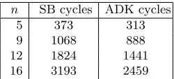
Finally results for an old 32-bit Intel Atom processor, using GCC version 4.8.4
n SB cycles ADK cycles
5 373 313
9 1068 888
12 1824 1441
16 3193 2459
Example Code
Here we present an example of the loop unrolled C code for the SB and ADK methods that we used in our tests. In this small example the number of limbsn
in xandy is 5. Code for carry propagation is included. In practise this code is automatically generated by a small utility program for any value ofn.
t y p e d e f i n t 6 4 t s m a l l ; t y p e d e f i n t 1 2 8 l a r g e ; #d e f i n e B 61 // b i t s i n r a d i x #d e f i n e M ( ( ( s m a l l )1<<B)−1) // Mask
v o i d sbmul5 ( s m a l l ∗x , s m a l l ∗y , s m a l l ∗z ) {
l a r g e t , c ;
t =( l a r g e ) x [ 0 ]∗y [ 0 ] ; z [ 0 ] = ( s m a l l ) t&M; c=t>>B ;
t=c +( l a r g e ) x [ 1 ]∗y [ 0 ] + ( l a r g e ) x [ 0 ]∗y [ 1 ] ; z [ 1 ] = ( s m a l l ) t&M; c=t>>B ;
t=c +( l a r g e ) x [ 2 ]∗y [ 0 ] + ( l a r g e ) x [ 1 ]∗y [ 1 ] + ( l a r g e ) x [ 0 ]∗y [ 2 ] ; z [ 2 ] = ( s m a l l ) t&M; c=t>>B ; t=c +( l a r g e ) x [ 3 ]∗y [ 0 ] + ( l a r g e ) x [ 2 ]∗y [ 1 ] + ( l a r g e ) x [ 1 ]∗y [ 2 ] + ( l a r g e ) x [ 0 ]∗y [ 3 ] ;
z [ 3 ] = ( s m a l l ) t&M; c=t>>B ; t=c +( l a r g e ) x [ 4 ]∗y [ 0 ] + ( l a r g e ) x [ 3 ]∗y [ 1 ] + ( l a r g e ) x [ 2 ]∗y [ 2 ] + ( l a r g e ) x [ 1 ]∗y [ 3 ]
+( l a r g e ) x [ 0 ]∗y [ 4 ] ; z [ 4 ] = ( s m a l l ) t&M; c=t>>B ;
t=c +( l a r g e ) x [ 4 ]∗y [ 1 ] + ( l a r g e ) x [ 3 ]∗y [ 2 ] + ( l a r g e ) x [ 2 ]∗y [ 3 ] + ( l a r g e ) x [ 1 ]∗y [ 4 ] ;
z [ 5 ] = ( s m a l l ) t&M; c=t>>B ; t=c +( l a r g e ) x [ 4 ]∗y [ 2 ] + ( l a r g e ) x [ 3 ]∗y [ 3 ] + ( l a r g e ) x [ 2 ]∗y [ 4 ] ; z [ 6 ] = ( s m a l l ) t&M; c=t>>B ; t=c +( l a r g e ) x [ 4 ]∗y [ 3 ] + ( l a r g e ) x [ 3 ]∗y [ 4 ] ; z [ 7 ] = ( s m a l l ) t&M; c=t>>B ;
t=c +( l a r g e ) x [ 4 ]∗y [ 4 ] ; z [ 8 ] = ( s m a l l ) t&M; c=t>>B ; z [ 9 ] = ( s m a l l ) c ;
}
v o i d adkmul5 ( s m a l l ∗x , s m a l l ∗y , s m a l l ∗z ) {
l a r g e t , s , c , d [ 5 ] ; d [ 0 ] = ( l a r g e ) x [ 0 ]∗y [ 0 ] ; d [ 1 ] = ( l a r g e ) x [ 1 ]∗y [ 1 ] ; d [ 2 ] = ( l a r g e ) x [ 2 ]∗y [ 2 ] ; d [ 3 ] = ( l a r g e ) x [ 3 ]∗y [ 3 ] ; d [ 4 ] = ( l a r g e ) x [ 4 ]∗y [ 4 ] ;
s=d [ 0 ] ; t=s ; z [ 0 ] = ( s m a l l ) t&M; c=t>>B ;
s+=d [ 1 ] ; t=c+s +( l a r g e ) ( x [ 1 ]−x [ 0 ] )∗( y [ 0 ]−y [ 1 ] ) ; z [ 1 ] = ( s m a l l ) t&M; c=t>>B ; s+=d [ 2 ] ; t=c+s +( l a r g e ) ( x [ 2 ]−x [ 0 ] )∗( y [ 0 ]−y [ 2 ] ) ; z [ 2 ] = ( s m a l l ) t&M; c=t>>B ; s+=d [ 3 ] ; t=c+s +( l a r g e ) ( x [ 3 ]−x [ 0 ] )∗( y [ 0 ]−y [ 3 ] ) + ( l a r g e ) ( x [ 2 ]−x [ 1 ] )∗( y [ 1 ]−y [ 2 ] ) ;
z [ 3 ] = ( s m a l l ) t&M; c=t>>B ; s+=d [ 4 ] ; t=c+s +( l a r g e ) ( x [ 4 ]−x [ 0 ] )∗( y [ 0 ]−y [ 4 ] ) + ( l a r g e ) ( x [ 3 ]−x [ 1 ] )∗( y [ 1 ]−y [ 3 ] ) ;
z [ 4 ] = ( s m a l l ) t&M; c=t>>B ;
s−=d [ 0 ] ; t=c+s +( l a r g e ) ( x [ 4 ]−x [ 1 ] )∗( y [ 1 ]−y [ 4 ] ) + ( l a r g e ) ( x [ 3 ]−x [ 2 ] )∗( y [ 2 ]−y [ 3 ] ) ; z [ 5 ] = ( s m a l l ) t&M; c=t>>B ; s−=d [ 1 ] ; t=c+s +( l a r g e ) ( x [ 4 ]−x [ 2 ] )∗( y [ 2 ]−y [ 4 ] ) ; z [ 6 ] = ( s m a l l ) t&M; c=t>>B ; s−=d [ 2 ] ; t=c+s +( l a r g e ) ( x [ 4 ]−x [ 3 ] )∗( y [ 3 ]−y [ 4 ] ) ; z [ 7 ] = ( s m a l l ) t&M; c=t>>B ; s−=d [ 3 ] ; t=c+s ; z [ 8 ] = ( s m a l l ) t&M; c=t>>B ;
Application to Montgomery’s REDC function
This well known method carries out reduction modulo m where field elements are first converted ton-residue form by multiplying them byb−nmodm, where
bn is larger than, and co-prime to, m. Assume that a product of a pair of n
-residues is to be reduced modulo m, and that the value of w = −1/mmodb
is precalculated. The following ADK-based method carries out the reduction. This function may be tightly combined with that of algorithm (1) to provide an integrated modular multiplication/squaring function z = xymodm for n -residues, where eachzi is processed as soon as it is calculated.
Algorithm 2ADK algorithm for the REDC function
Input: Modulusmof degreen, radixb= 2t, precalculatedw=−1/mmodb
Input: z= [z0, . . . , z2n−2,0], wherezi∈[0, b2−1]
Output: r= [r0, . . . , zn−1], whereri∈[0, b−1] andr=zb−n modm
1: functionADKredc(z)
2: t←z0
3: v0 ←twmodb
4: t←t+v0m0
5: c←z1+t/b
6: s←0
7: fork←1 ton−1do
8: t←c+s+v0mk
9: fori←1 +⌊k/2⌋tok−1do
10: t←t+ (vi−vk−i)(mk−i−mi)
11: end for
12: vk←twmodb
13: t←t+vkm0
14: c←zk+1+t/b
15: dk ←vkmk
16: s←s+dk
17: end for
18: fork←nto 2n−2do
19: t←c+s
20: fori←1 +⌊k/2⌋ton−1do
21: t←t+ (vi−vk−i)(mk−i−mi)
22: end for
23: rk−n←tmodb
24: c←zk+1+t/b
25: s←s−dk−n+1
26: end for
27: rn−1 ←cmodb
28: returnr
This implementation includes full carry propogation. Observe that divisions and remainders modulo b are carried out using simple shift and masking oper-ations as b is a power of 2. As is well known the output of this algorithm may require one extra subtraction of the modulus m to get a fully reduced result. However in many contexts field elements will not need to be immediately fully reduced. The number of muls and adds compared with a straight-forward SB-based implementation is given in Table (7) In some cases the constant wmay be equal to 1, which allows some extra saving. Working code in a variety of languages can be found in thebigmodule here2.
muls adds
SB n(n+ 1) 2n2+ 4n−2
ADK (n2+ 5n−2)/2 2n2+ 10n−8 Table 7.REDC Complexity
2