Dynamic project selection

BIROn - Birkbeck Institutional Research Online

Pancs, R. and Nikandrova, Arina (2015) Dynamic project selection. Working

Paper. Birkbeck College, University of London, London, UK.

Downloaded from:

Usage Guidelines:

Please refer to usage guidelines at or alternatively

ISSN 1745-8587

Department of Economics, Mathematics and Statistics

BWPEF 1505

Dynamic Project Selection

Arina Nikandrova

Birkbeck, University of London

Romans Pancs

University of Rochester

April 2015

Birkb

eck Worki

ng

Papers i

n

Economi

cs

&

Fina

Dynamic Project Selection

Arina Nikandrova and Romans Pancs

April 2015

Abstract

We study a normative model of an internal capital market, used by a company

to choose between its two divisions’ pet projects. Each project’s value is initially

un-known to all but can be dynamically learned by the corresponding division. Learning

can be suspended or resumed at any time and is costly. We characterize an

inter-nal capital market that maximizes the company’s expected cash flow. This market

has indicative bidding by the two divisions, followed by a spell of learning and then

firm bidding, which occurs at an endogenous deadline or as soon as either division

requests it.

Keywords: internal capital market, irreversible project selection

JEL codes: D82, D83, G320, G310.

∗_{Nikandrova ([email protected]) is at Birkbeck; Pancs ([email protected]) is at the University}

1

Introduction

A corporate finance textbook (e.g., Webster, 2003, Chapter 12) would recommend that a

company invest in a project if and only if the project’s internal rate of return exceeds the

cost of capital. If companies operated in this manner, their investment decisions would be

independent across projects within the company, conditional on the projects’ cash flows.

In practice, such independence is an exception rather than the rule (Ozbas and

Scharf-stein,2010).

Investment decisions can be interdependent for two reasons: projects may be mutually

exclusive, or internal capital, used to finance these projects, may be scarce. We use the

term “internal capital market” to describe a project-selection mechanism that deals with

either situation. We are interested in the design of an optimal internal capital market.

We focus on problems in which project values are initially unknown but can be learned

over time. Before deciding which project to finance, a company carries out due diligence

on each project. If due diligence were unnecessary or infeasible, optimal project selection

would be trivial because the company would immediately choose the project with the

highest expected value, without any deliberation.

The situation in which Universal Music Group found itself in 2011 fits our model’s

environment exactly. Universal was considering two alternative projects: the purchase of

EMI Music and the purchase of Warner Music Group.1 Purchasing both was infeasible, if

only because of antitrust concerns. Assessing the profitability of each purchase required

costly due diligence by the teams of lawyers, consultants and accountants, to evaluate

music catalogs, potential synergies, and antitrust risks.

EMI is based in London; Warner Music is based in New York. Universal

(headquar-tered in Santa Monica) also happens to have two divisions: one in London and one in

New York. Universal could charge the London division with carrying out due diligence

1_See

pertaining to the purchase of EMI and could charge the New York division with carrying

out due diligence pertaining to the purchase of Warner Music. Our first question asks

how Universal should orchestrate its divisions’ due diligence to maximize its expected

cash flow.

The example of Universal carries one further complication. The London division

fa-vors buying EMI because this purchase would increase the influence of the London

di-vision. The New York division similarly favors buying Warner Music. If Universal’s

headquarters cannot monitor each division’s due diligence, then each division is likely

to be strategic when deciding whether to follow the headquarters’ recommendations

re-garding due diligence (moral hazard) and when deciding whether to report truthfully the

outcomes of its due diligence (adverse selection). Hence, our second question asks how

the optimal policy can be implemented in the presence of both moral hazard and adverse

selection.

To address the two design questions raised above, we study Universal’s problem in an

auction-like environment. HQ (the headquarters) allocates an item (the requisite funds

to pursue an acquisition) to one of two divisions, denoted by D1 and D2. The value

of each division’s project (the profitability of the acquisition) is either 0 or 1 and is

dis-tributed independently across the two divisions. Initially, each division has a belief about

its project’s value and revises this belief as it learns (carries out due diligence).

Time is continuous, and the time horizon is infinite. At each instant, each division can

learn at a cost. A division’s learning affects the arrival intensity of “good news,” which

reveals the project’s value to be 1. The alternative, “no news,” means that the project’s

value can be either 0 or 1 and causes the division to revise its value estimate downward.

HQ maximizes the expected cash flow, defined as the expected value of the winning

project net of both divisions’ expected cumulative costs of learning. Assuming HQ can

directly control each division’s learning, observe learning outcomes, and select the

0.0

0.2

0.4

0.6

0.8

1.0

0.0

0.2

0.4

0.6

0.8

1.0

q

q

I

Division 1

learns

Division 2

learns

Division 2

wins

Division 1

wins

Division 1

learns

Division 2

learns

both divisions learn

x

₁

x

₂

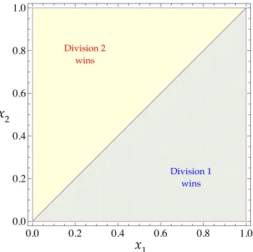
Figure 1: An optimal policy’s prescription for each pair(x1,x2) of the project’s expected

values.

problem’s solution—an optimal policy—is this paper’s first contribution. The second

contribution is the optimal policy’s implementation in the presence of moral hazard and

adverse selection.

Figure1summarizes an optimal policy when the cost of learning is sufficiently small.2

This optimal policy is stationary and prescribes, for every pair(x1,x2)of the two projects’

expected values, whether either division should win immediately, and if not, which

divi-sion should learn. Normalizingx2 ≥x1, four prescriptions are possible:

1. Division 2 wins immediately

D2wins immediately wheneverx1andx2are either both close to 0 or both close to 1.

In this case, there is little uncertainty about each project’s value, and so learning is

not worth the cost. D2 also wins immediately whenever x2 is substantially larger

thanx1. In this case, there is little uncertainty about the fact that the value of project 2

exceeds the value of project 1, so learning is unlikely to affect the decision regarding

which project to select and hence is suboptimal.

2. Division 2 learns

D2 learns when x1 and x2 are close to each other (so that which project is more

valuable is highly uncertain), and when bothx1andx2are far away from 0 and 1 (so

that each project’s value is highly uncertain). In this case, the need for information

is so great that it is worthwhile to ask D2 to learn first, and to plan on also asking

D1to learn later if D2does not observe good news. Asking D2to learn without ever

planning to ask D1to learn is suboptimal, as is explained below.

D2’s learning is more informative than D1’s, which suggests that asking D2to learn

may be optimal. Indeed, because x2 > x1, D2stands a higher chance of observing

good news than D1 does. At the same time, a spell of no news leads to a rapid

downward revision of D2’s belief because a likely event—the arrival of good news—

has failed to occur. Either way, as D2learns, its belief changes fast.

Asking only D2 to learn, without planning to ask D1 to learn later on, amounts to

committing to choose D2’s project. Such a commitment is suboptimal because D2’s

belief is a martingale, and consequently, D2’s learning entails costs, but does not

affect the (ex-ante) expected value of D2’s project. By contrast, if D2’s learning, with

positive probability, is followed by D1’s learning, then the selected project’s identity

is contingent on the outcomes of learning, thereby justifying learning.

Both divisions learn simultaneously if (i)x1 =x2(i.e., which project is more valuable

is unclear), (ii) x1 and x2 are sufficiently large (i.e., learning by either division is

rather informative), and (iii) x1 and x2 are bounded away from 0 and 1 (i.e., each

project’s value is highly uncertain).

4. Division 1 learns

D1 learns whenever the values ofx1and x2 are complementary to those described

in scenarios1–3. In this case, by having D1learn, HQ bets on having D1observe the

good news. HQ is “insured” by D2, which does not learn, and whose project can be

selected if D1observes no news.

We show that the described optimal policy is implementable in the presence of moral

haz-ard and adverse selection. That is, the prescriptions of the optimal policy coincide with

equilibrium outcomes of a carefully constructed dynamic game, called optimal auction

game. In this game, each division learns privately and hence must be motivated to

con-form with the optimal policy. The optimal auction begins with indicative bidding: each

division publicly announces a real number, which does not directly affect the division’s

payment or the chances of getting its project selected. HQ uses the announced indicative

bids to compute the firm-bidding deadline, which HQ then publicly announces. Until the

deadline, each division can learn and, irrespective of whether it is learning, may be asked

by HQ to pay a fee for the right to remain in competition. At any time, either division

may request early firm bidding. Firm bidding takes the form of the second-price auction,

which determines the divisions’ payments and the winning project.

The fees and the firm-auction rules are chosen to ensure that each division pays the

“externality” that its participation imposes on the other division, by analogy to a

Vickrey-Clarke-Groves mechanism. Each division thus becomes a “residual claimant” to the cash

flow. As a result, at equilibrium, each division’s indicative bid equals its prior belief about

its project’s value. Furthermore, each division learns as prescribed by the optimal policy

bid is its final belief about its project’s value. Thus, the highest expected-value project is

selected.

Our paper contributes to two literatures: corporate finance literature on internal

cap-ital markets and economic theory literature on irreversible project selection in the

pres-ence of uncertainty, including the literature on auctions with information acquisition. The

assumptions underlying our model of the internal capital market are motivated by the

vision described byStein(1997).3 In particular, because internal capital is scarce (e.g.,

be-cause of informational frictions associated with raising outside capital), not all profitable

projects can be financed and so HQ must ration. At the same time, even unprofitable

projects may end up being financed (e.g., because of HQ’s empire-building tendencies),

and so HQ invests all available internal capital. Accordingly, we assume that HQ selects

exactly one project.

Existing literature on internal capital markets is predominantly positive. Among the

positive models, in addition to Stein (1997), are Harris and Raviv (1996), Rajan et al.

(2000), Scharfstein and Stein (2000), de Motta (2003), andInderst and Laux (2005). The

only normative dynamic model of an internal capital market that we are aware of is that

ofMalenko(2012). Whereas our focus is on learning about, and selection from, two given

projects, Malenko (2012) studies selection from dynamically arriving projects and does

not model learning.

The economic theory literature on irreversible project selection can be interpreted to

model internal capital market. The real-option approach, exemplified by the work of

Dixit and Pindyck (1994), assumes that the values of projects evolve exogenously. We

extend their approach to situations in which these values evolve endogenously, as a result

of learning. Learning is the focus of multi-armed bandit problems (Bolton and Harris,

1999;Keller et al.,2005;Klein and Rady,2010). Bandit problems model reversible project

selection because a selected arm can be unselected as new information arrives. In the 3_{For a textbook introduction to internal capital markets, seeTirole(2006, Section 10.5) andGertner and}

bandit problems in which no new information can ever justify unselecting an arm (and so

investment irreversibility is irrelevant), there is no way to incorporate the cost of learning

in a manner consistent with our model.4

Persico(2003),Compte and Jehiel(2007),Crémer et al.(2009),Shi(2012), andKrähmer

and Strausz (2011) analyze information acquisition in auctions, but do not investigate

situations in which learning can occur over an infinite horizon, information is cumulable

over time, and no structure is imposed on the timing of learning. The richness of the set

of admissible learning policies distinguishes our model and leads to novel insights. For

example, the insight that sometimes it is optimal for the higher-expected-value division

to learn would be lost in a model with a one-off chance to learn. The richness of the policy

set comes at a cost; we work with a rather special, good-news, learning technology.

Athey and Segal (2007) andBergemann and Välimäki (2010) are our inspirations for

the auction implementation of the optimal policy.

The rest of the paper is structured as follows. Section 2 describes the environment.

Section3conjectures and informally justifies an optimal policy. Section4verifies the

con-jecture by appealing to the viscosity-solution techniques. Section5describes the optimal

policy’s implementation in a dynamic auction. Section6concludes.

2

Model

Time is continuous and is indexed byt≥0. The time horizon is infinite.

Valuations

HQ holds an indivisible item, which it values at zero. HQ allocates this item to one of

two divisions, indexed byi_{∈ N ≡ {}1, 2_}and denoted by Di. Di’s valuationvi ∈ {0, 1}is

4_{The challenge within the bandit framework is to make the cost of learning vanish once an irreversible}

a random variable with Pr_{vi =1} = Xi(0), for some prior beliefXi(0) ∈ [0, 1], i ∈ N. Valuationsv1andv2are statistically independent.

Learning

At any timet, each Di can acquire information about vi, orlearn. Let ai be the indicator function with values in {0, 1} such that ai(t) = 1 indicates that Di learns at time t. The cumulative cost of learning incurred by Di from time 0 to timetisc

Rt

0 ai(s)ds, for some

cost parameterc >0.

Di’s learning process{ai(t)| t≥0}, denoted by ai, controls the arrival-intensity pro-cess_{λai(t)vi |t ≥0}of a Poisson process N_iai(t) |t ≥0 that has N_iai(0) = 0, where

λ > 0 is interpreted as the precision of learning. The event when N_iai(t) is incremented is called good news(about vi). The event when N_iai(t) is not incremented is called no

news. Because the event Nai

i (t) > 0 can occur only if vi = 1, the good news reveals

vi =1. Processes N₁a1 and N2a2 are assumed to be independent.

DefineXai

i (t), Di’s time-ttype, orbelief, to be the expectation ofviconditional on the information revealed up to timetand on some learning process ai:

Xai

i (t)≡E

vi |

Nai

i (s) |0≤s ≤t =E

vi | N_iai(t)

.

The last equality in the display above obtains because Nai

i (t)summarizes all the history that is relevant for learning about vi. For any learning-process profile a ≡ (a1,a2), the

tuple Xa(t) ≡ Xa1

1 (t),X

a2

2 (t)

is a time-ttype profile. By construction (by the Law of

Iterated Expectations), the processXais a martingale.

The Evolution of Types

For anyt andt0 > t, Di’s typeX_iai(t0) is derived fromX_iai(t)by application of the Bayes rule. According to the Bayes rule, Nai

i (t0) > 0 impliesX ai

i (t0) = 1, whereas N ai

implies

Xai

i (t0) 1−Xai

i (t0)

= X

ai

i (t) 1−Xai

i (t)

e−λR_tt0ai(s)ds_{. (1)}

For future reference, let us describe the stochastic type process Xai

i in its differential form. BecauseXai

i is not conditional onvi, it is convenient to define the good-news Pois-son process ˜Nai

i whose arrival intensity is also unconditional, and equals λai(t)X ai

i (t). The stochastic differential equation forXai

i becomes

dXai

i (t) = 1−X ai

i (t)

d ˜Nai

i (t)−λai(t)Xiai(t) 1−X ai

i (t)

dt (2)

subject to Xai

i (0) = Xi(0). The differential representation in (2) is a difference of two terms. The first term is the upward jump in the belief caused by the arrival of good news.

The second, negative, term is the downward revision of the belief caused by the failure of

the good news to arrive during learning; the magnitude of this revision follows from the

Bayes formula in (1).

An Optimal Policy

The environment is stationary, and so no generality is lost by focusing on stationary

poli-cies. A (stationary) policyis a tuple(α,τ), where the learning policy α ≡ (α1,α2) maps

a type profile x _≡ (x1,x2) into learning decisions (α1(x),α2(x)) in {0, 1}2\(0, 0), and

where τ is the stopping time that designates when the item is allocated to the

highest-type division.5 A policy(α,τ)induces the type process denoted by{Xα,τ(t) | t≥0}. A policy (α,τ) is admissible if the learning process {α(X(t))| t≥0}, induced by

the learning policy α, is predictable and integrable,6 and if, for every i ∈ N and every

5_{No generality is lost by requiring that at least one division learn at any time until the item has been}

allocated;(α1(x),α2(x))6= (0, 0).

6_{A continuous-time stochastic process ispredictableif it is measurable with respect to the}

σ-algebra

generated by all left-continuous adapted processes. In the current setting, predictability means that the induced learning process is adapted with left-continuous paths; that is, at everyt,α(X(t)) =α(X(t−)),

where X(t−) ≡ lims→t,s<tX(s). In other words, when armed with an admissible policy(α,τ) and

Xi(0) ∈ [0, 1], the stochastic differential equation (2) has a unique strong solution.7 A policy(α,τ)and an initial type profilexinduce the expectedcash flow

J(x,α,τ)≡E "

max i∈N

Xα,τ

i (τ) −c

∑

Z _τ

0 αi(X

α,τ_{(s))ds| X}α,τ_{(0) = x} #

. (3)

For every initial type profilex, thevalue functionφis defined by

φ(x) ≡sup α,τ

J(x,α,τ), (4)

where the maximization is over all admissible policies. An optimal policy (α∗,τ∗) is

defined to satisfyφ(x) = J(x,α∗,τ∗)for allx.

3

A Conjectured Optimal Policy and Value Function

An optimal policy and the induced value function are conjectured by appealing to HJBQVI

(Hamilton-Jacobi-Bellman Quasi-Variational Inequality), a continuous-time analogue of

the Bellman equation. The conjecture is subsequently verified using the viscosity

ap-proach.

Define the effective cost ˆc _≡c/λ, the cost of learning per unit of precision. The optimal

policy will be shown to depend on c and λ only through ˆc. Inspired by the divisions’

symmetry (except for their prior beliefs), a symmetric optimal policy and a symmetric

value function are conjectured. Hence, whenever the description of a policy or a value

function is restricted to the case in which x2 ≥ x1, the symmetric case x2 < x1 follows

immediately.

foresee, however, the jump inXthat may occur att(Xis not left continuous) or whether the item will be allocated at timet(even though adapted,τneed not be predictable).

7_{Protter(1990, Chapter V) discusses the conditions for existence and uniqueness of strong solutions to}

3.1

HJBQVI

Define an open convex set Ω ≡ (0, 1)2, whose closure is ¯Ω. On the boundary ∂Ω of

Ω, immediate allocation is trivially optimal; the identity of the division with the highest

valuation is known;x _∈ ∂Ωimpliesφ(x) = max{x1,x2}. It remains to findφonΩ.

Any candidate value function, denoted by u, must satisfy HJBQVI, which can be

de-rived as the limit of the Bellman equation for the corresponding discrete-time model as

the length of each time period goes to zero. This derivation is standard and gives

min i∈N

ˆ

c+xi(1−xi)

∂u(x) ∂xi −

xi(1−u(x)),u(x)−xi

=0, x _∈ Ω (5)

and theboundary condition

u(x) =max

i∈N {xi}, x ∈ ∂Ω. (6)

The quasi-variational-inequality (QVI) component of (5) isu(x) ≥max_{x1,x2}. QVI

requires that the value provided by a candidate value functionube at least as high as the

value that can be obtained from immediately allocating the item.

The Hamilton-Jacobi-Bellman (HJB) component of (5) is

min i∈N

ˆ

c+xi(1−xi)

∂u(x) ∂xi −

xi(1−u(x))

=0, x _∈ Ω.

HJB requires that, whenever u suggests the suboptimality of immediate allocation (i.e.,

u(x) > max{x1,x2}), some division, say, Di, learns, andusatisfies the no-arbitrage con-dition

c+ λxi(1−xi)

∂u(x) ∂xi

| {z }

payoff revision due to no news

= λxi(1−u(x))

| {z }

payoff revision due to good news

, x_∈ Ω. (7)

contin-uation value in response to that decline. The right-hand side of (7) is the expected arrival

intensity λxi of good news times the discrete change 1−u(x)in the continuation value in response to the arrival of good news. Thus, condition (7) is essentially definitional; it

requires any candidate value function to promise zero expected change in the payoff from

following a candidate optimal policy. In other words, any expected change in the future

payoff must be incorporated into the current expected payoff.

To admit the possibility that a value function is nondifferentiable on a null set (which

will be the case in our problem), we define a solution concept that ignores the points of

nondifferentiability.

Definition 1. A functionu∗ : Ω →Ris ageneralized solutionof, org-solves, HJBQVI if

u∗satisfies HJBQVI almost everywhere inΩ.

Our conjecture for φ on Ω is denoted by F. It is constructed to g-solve HJBQVI and

satisfy the boundary condition (6). In principle, multiple functions may g-solve HJBQVI

subject to the boundary condition. The constructed conjecture is recommended by the

economic intuition for the underlying policy and, eventually, the verification argument.

The qualitative features of Fvary with the magnitude of ˆc, and so three cases are

distin-guished.

3.2

Learning Is Prohibitively Costly:

c

ˆ

_≥

c

The Conjecture

It is natural to conjecture that if the cost of learning exceeds some threshold, then, at any

type profilex, it will be suboptimal to ask any division to learn. Instead, the item will be

optimally allocated immediately to the highest-type division, as is illustrated in Figure2.

The associated conjectured value function is

0.0

0.2

0.4

0.6

0.8

1.0

0.0

0.2

0.4

0.6

0.8

1.0

q

q

Division 2

wins

Division 1

wins

x

₂

x

₁

Define the relevant effective-cost threshold to bec2= 1₂, or equivalently,

c2 ≡inf

c0 ≥0| inf

0≤x1≤x2≤1

c0−x1(1−x2) ≥0

. (8)

Thresholdc2in (8) is motivated by the infinitesimal look-ahead rule (Ross,1970, Section

9.6), which is a continuous-time counterpart of the one-step look-ahead rule in

discrete-time stopping problems. The thresholdc2in (8) is the smallest (effective) costc0such that,

at any type profilex with x2 ≥ x1 (which is a normalization), HQ prefers allocating the

item immediately to the highest-type division (D2) to having the lowest-type division (D1)

learn forδ →0 units of time, at cost λc0δ, and only then allocating the item to whomever

by then has been revealed as the highest-type division. The revealed highest-type division

is D1if and only if it observes the good news, which occurs with probabilityx1 1−e−λδ

.

With the complementary probability, D2of typex2remains the highest-type division. The

inequality associated with HQ’s stated preference is

x2 ≥ −λc0δ+x1

1₋e−λδ₊₁

−x1

1₋e−λδ_x

2, (9)

which leads to the inequality in (8) whenδ →0.

The Conjecture G-Solves HJBQVI

Lemma 1. Suppose that learning is prohibitively costly, orcˆ≥c2. The conjectured value function

F(x) =max{x1,x2}g-solves HJBQVI subject to the boundary condition.

Proof. SubstitutingFinto HJBQVI (5) and recalling the conventionx2 ≥x1yields

min{cˆ−x1(x1−x2), 0} =0, x ∈ Ω,

which is implied by ˆc_≥c2and the definition ofc2in (8).

by Definition1, Fg-solves HJBQVI.

It is immediate that Fsatisfies the boundary condition (6).

3.3

Learning Is Moderately Costly:

c

≤

c

ˆ

<

c

The Conjecture

If the (effective) cost ˆc of learning is below the threshold c2, defined in (8), asking some

division to learn is optimal, which follows from the infinitesimal look-ahead perturbation

formerly ruled out by (9). Further, it is natural to conjecture that any type profile x at

which learning occurs hasx1andx2close to each other, so that it is quite uncertain which

division has a higher value, and has bothx1andx2sufficiently far away from 0 and 1, so

that there is considerable uncertainty about each division’s value.

Which division learns depends on x and ˆc. For now, we focus on the case in which

c1 ≤ cˆ < c2, wherec1 ≈0.047. Then, whenever learning occurs, the lower-type division

learns. The thresholdc1is the unique solution of8

log(1−

√_c

1)2

c1

= 2

1−√c1

. (10)

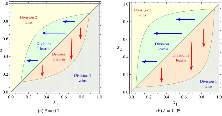
The conjectured optimal policy is illustrated in Figure 3. To demarcate the set of type

profiles at which D1 learns—the lens-shaped region in the figure—normalize x2 ≥ x1.

Define a type threshold for D1as a function of D2’s type:

b(x2) ≡ cˆ

1₋x2

. (11)

In Figure3, D1learns if x1 > b(x2); otherwise, D2wins immediately. When D1 learns, it

wins if and only if it observes the good news. Becauseb is increasing in ˆc, the lower the

cost of learning, the larger the set of type profiles at which some division learns.

8_{Equation (10) admits no interpretation by inspection and emerges from a condition that ensures that}

0.0 0.2 0.4 0.6 0.8 1.0 0.0

0.2 0.4 0.6 0.8 1.0

q1 q2

Division 1 learns

Division 2 learns Division 2

wins

Division 1 wins x₂

x₁

(a) ˆc=0.1.

0.0 0.2 0.4 0.6 0.8 1.0 0.0

0.2 0.4 0.6 0.8 1.0

q₁

q₂ Division 1 _learns

Division 2 learns Division 2

wins

Division 1 wins x₂

x₁

(b) ˆc=0.05.

Figure 3: The optimal policy’s prescription for each type profile when the learning cost is moderate; c1 ≤ cˆ < c2. Within the lens-shaped region, one of the divisions learns. The

In order to see the intuition for why the lower-type division, say D1, is the one that

learns, note that asking D1 to learn amounts to betting on D1’s observation of the good

news. This bet’s upside is to see D1 observe the good news and then let it win. The bet’s

downside is bounded by D2’s type. If D1 observes no news for a sufficiently long period

of time, HQ lets D2win. Because D2 does not learn, its type does not deteriorate and so

ensures against the downward revisions of D1’s type.

The rest of the subsection is concerned with demonstrating, in Lemma 3, that the

conjectured value function F associated with the described conjectured policy g-solves

HJBQVI. In the course of this demonstration, the origins of the boundarybin (11) and of

the thresholdc1in (17) are explained.

The Conjecture G-Solves HJBQVI

A critical element in the proof of the conjectured policy’s optimality is an optimal

stop-ping problem referred to as the V-auxiliary problem, defined in (11). This problem is

solved by b of (11). In this problem, consistent with the conjectured optimal policy, D1,

the lower-type division, learns up to some optimally chosen deadline t ≥ 0. At t or as

soon as D1 observes the good news, learning stops, and the division with the highest

revised type wins. The value of the V-auxiliary problem is denoted by V and will be

observes the good news,” the functionVis defined

V(x) ≡ sup t≥0

       x1

1−e−λt

| {z }

payoff from D₁’s winning

+x2

1−x1

1−e−λt

| {z }

payoff from D₂’s winning

− x1c

Z t

0 sλe

−λs_ds

| {z }

expected cost of learning ifF

− ct1₋x1

1₋e−λt

| {z }

expected cost of learning if notF

         = sup

t≥0

1−(1−x2)

1−x1

1−e−λt

−c

(1−x1)t+x1

1₋e−λt λ

,(12)

where the last equality is obtained by computing the integral and simplifying.

It is convenient to change variables in (12). Instead of maximizing over the deadline

t, maximize over D1’s corresponding threshold type, denoted byz. The relationship

be-tween the deadline and the threshold type is found by the Bayes rule, as in (1):

z

1₋z = x1

1₋x1

e−λt_.

Substitutingzfrom the display above into the expression forV in (12) yields

V(x) _≡ sup z∈[x1,0)

1₋(1−x1) (1−x2)

1−z −cˆ(1−x1) [ϕ(x1)−ϕ(z)]

, (13)

where

ϕ(s)≡ s

1₋s +ln s

1₋s, s ∈(0, 1).

In (13), the term 1−(1−x1) (1−x2)/(1−z)is the expected payoff from eventually

al-locating the item, either to D1 (as soon as D1 observes the good news) or to D2 (if D1

never observes the good news). The term ˆc(1−x1) [ϕ(x1)−ϕ(z)]is the expected cost of learning.

0.0

0.2

0.4

0.6

0.8

1.0

0.0

0.2

0.4

0.6

0.8

1.0

q

q

_x

2

x

₁

ˆ

V

I

b

(

x

₂

)

Figure 4: Each of the depicted setsI and ˆV depends on ˆcand collects the type profiles at which the conjectured optimal policy makes identical prescriptions. The sets_I and ˆ_V are separated by the functionb.

type set

ˆ

V ≡ nx ∈ [0, 1]2 | b(x2) <x1 ≤x2

o

, (14)

and the complementary set

I ≡ nx _∈ [0, 1]2 | x1 ≤x2

o

Vˆ. (15)

These sets are depicted in Figure4.

if x ∈ I, and

V(x) =1−(1−x1) (1−x2)

1−b(x2) −

ˆ

c(1−x1) [ϕ(x1)−ϕ(b(x2))] (16)

if x _∈Vˆ. The policy that achieves V has D2win immediately if x ∈ I and has D1learn if x ∈ Vˆ.

Proof. The thresholdb(x2), defined in (11), is derived using the infinitesimal look-ahead

rule for optimal stopping problems (Ross, 1970, Section 9.6). According to this rule, at

any type profilex, it is optimal for D1to learn if and only if learning for amountδ →0 of time and then allocating the item to the division with the highest revised type delivers a

weakly higher cash flow than immediately allocating the item to the higher-type division.

Assuming (and verifying shortly) that the infinitesimal look-ahead rule applies, D1

learns ifx _{∈ V}ˆ, and D2wins immediately ifx ∈ I. The threshold functionbemerges from

the indifference condition. Whenx1 =b(x2), HQ is indifferent between (i) allocating the

item to D2and (ii) having D1learn forδ →0 units of time and then allocating the item to the division with the highest revised type. This indifference condition is

x2 = lim

δ→0

−cδ+b(x2)

1₋e−λδ₊h₁

−b(x2)

1₋e−λδi_x

2

.

Computing the limit and simplifying gives b as defined in (11). The value function in

(16) is then derived from (13) assuming that the infinitesimal look-ahead rule applies as

described.

By Theorem 9.3 of Ross(1970), to ascertain that the infinitesimal look-ahead rule

in-deed applies, one must verify that_I is closed in the sense thatx _{∈ I} implies that, for any

x0₁ < x1, (x10,x2) ∈ I. The set I is indeed closed, by inspection of (14) and (15). Hence,

the infinitesimal look-ahead rule applies, and the desired result follows.

The thresholdc1in (17) emerges from the condition that, for any x ∈ Vˆ, rules out the

of time before the conjectured optimal policy is resumed. This deviation can be verified

to be unprofitable if and only if ˆc ≥c1, where

c1 ≡ min

c0 _≥0| min

0≤x1≤x2≤1

Φ x,c0

≥0

(17)

for

Φ(x, ˆc) ≡ 1−x2(1−x1) (ϕ(x1)−ϕ(b(x2))). (18)

The right-hand side of (18) depends on ˆc implicitly, through b(θ2) ≡ cˆ/(1−θ2). Here,

Φ is proportional to HQ’s payoff from having D1 learn as prescribed by the conjectured

policy less the payoff from asking D2 to learn forδ →0 and only then asking D1to learn

as prescribed by the conjectured policy. This payoff is nonnegative for all x ∈ Vˆ as long

as ˆc _≥ c1. LemmaB.1 of Appendix B proves that c1 defined in (17) can be equivalently

and more simply characterized as the unique solution of (10).

Lemma 3. Suppose that learning is moderately costly, or c1 ≤ cˆ < c2. The conjectured value

function F(x) = 1_{x∈Vˆ}V(x) +1_{x∈I}x2 g-solves HJBQVI and satisfies the boundary

condi-tion.

Proof. HJBQVI is verified by considering two cases: x∈ I andx ∈Vˆ.

1. Suppose x _{∈ I}, or equivalently, x1 ≤ b(x2), so thatF(x) = x2. As in the proof of

Lemma1, the implied HJBQVI equation is

min

i∈N {cˆ−x1(1−x2), 0} =0, x ∈ Ω

which holds true becausex1 ≤b(x2) = cˆ/(1−x2), byx ∈ I.

verified component by component of the min function:

min   

 

ˆ

c+x1(1−x1)∂V_∂x(₁x) −x1(1−V(x)),

ˆ

c+x2(1−x2)∂V_∂x(₂x) −x2(1−V(x)),V(x)−x2

  

 

=0.

(a) To show

ˆ

c+x1(1−x1)∂

V(x)

∂x1 −x1(1−V(x)) =0, (19)

differentiateVin (16) to obtain

∂V(x) ∂x1

= 1−x2

1₋b(x2)

+cˆ(ϕ(x1)−ϕ(b(x2)))−cˆ(1−x1)ϕ0(x1). (20)

Substitution of the above display and ofVinto (19) verifies the equality.

(b) The inequality V(x) ≥ x2 follows by “revealed preference,” that is, by

con-struction of the V-auxiliary problem.

(c) To show

ˆ

c+x2(1−x2)∂V(x)

∂x2 −

x2(1−V(x))≥0, (21)

apply the Envelope Theorem (Milgrom and Segal, 2002) to the definition ofV

in (16) to obtain

∂V(x) ∂x2 =

1−x1

1−b(x2).

Substituting the above display and (16) into (21), dividing by ˆc, and

substitut-ing the definition ofbyields an equivalent desired inequality:

Φ(x, ˆc)≥0, (22)

whereΦ is defined in (18). Because Φis increasing in ˆc, the inequality in (22)

holds for all admissible x if and only if ˆc is sufficiently large. Then, because

ˆ

definitive.

Fis non-differentiable only on a null subset of the 45-degree line in the type space. Hence,

by Definition1,Fg-solves HJBQVI, as desired. It is immediate that Fsatisfies the

bound-ary condition.

3.4

Learning Is Cheap:

c

ˆ

<

c

The Conjecture

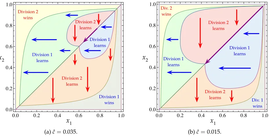
If the (effective) cost ˆc of learning falls below threshold c1, defined in (17), asking the

higher-type division to learn is no longer suboptimal. Intuitively, learning drives the

di-visions’ types apart, thereby helping HQ identify the highest-valuation division.

Learn-ing is faster for the higher-type division, say D2, which is more likely than D1to observe

the good news. If D2 observes the good news, its type jumps to 1. If D2 observes no

news, its type is revised substantially because an event deemed likely (the arrival of the

good news) has failed to occur. That is, in some informal sense, D2’s learning is more

informative than D1’s learning.

Because each division’s revised type is a martingale, the policy of asking only D2 to

learn and then selecting D2’s project regardless of the learning outcome does not affect the

project’s expected value but entails learning costs, and so cannot be optimal. Therefore,

D2’s learning can be optimal only if it is sufficiently long to potentially flip the ranking

of the divisions’ revised types. Lengthy learning can be optimal only if learning is

suffi-ciently cheap—which leads to the condition ˆc<c1—and only if the need for information

is sufficiently large. The need for information is large when the typesx1 andx2 are close

to each other (so that which project is more valuable is highly uncertain), when both x1

and x2 are far away from 0 and 1 (so that each project’s value is highly uncertain), and

whenx2is rather large (so that D2’s learning is rather informative).

0.0 0.2 0.4 0.6 0.8 1.0 0.0

0.2 0.4 0.6 0.8 1.0

q₁

q₂ Division 1

learns

Division 2 learns Division 2

wins

Division 1 wins Division 1

learns Division 2

learns

x₂

x₁

(a) ˆc=0.035.

0.0 0.2 0.4 0.6 0.8 1.0 0.0

0.2 0.4 0.6 0.8 1.0

q₁ q2 _{Division 1}

learns

Division 2 learns Div. 2

wins

Div. 1 wins Division 1

learns

Division 2 learns

x₂

x₁

(b) ˆc=0.015.

Figure 5: The optimal policy’s prescription for each type profile when the learning cost is small; ˆc < c1. Within the lens-shaped region (which encompasses the heart-shaped

heart-shaped region, the highest-type division learns. Elsewhere in the lens-shaped

gion, the lowest-type division learns. On the diagonal traversing the heart-shaped

re-gion, both divisions learn. If neither division learns, the highest-type division wins. The

boundary of the lens-shaped region is demarcated by functionbdefined in (11), as before.

The demarcation of the heart-shaped region is subtler and will be derived after additional

notation has been developed.

The Conjecture G-Solves HJBQVI

The economic intuition for D2’s occasional learning, supplied above, will be

comple-mented by a technical intuition. The notation required to formulate the conjectured

value function will be introduced along the way. The technical intuition can be

infor-mally viewed as the first step of a value-function-iteration-like procedure. Take the value

function in Lemma 3to be the initial guess for the value function for the case in which

ˆ

c <c1.

For every x _{∈ V}ˆ, Lemma 3 prescribes that D1 learn. This prescription induces the

value function that violates HJBQVI whenever ˆc < c1. In particular, inequality (22) in

Step2cof the lemma’s proof fails on thefailure set

F ≡ {x _| Φ(x, ˆc) <0}. (23)

Figure 6aillustrates the failure set. On and only on F, infinitesimal learning by D2

fol-lowed by D1’s learning is a profitable deviation from the policy in which only D1 learns

on ˆV. The described identification of the failure set would be the first step in the

“value-function iteration process.”

Lemma6“patches” the failure setF by making D2learn on a certain set, calledpatch,

which is a strict superset of_F, as is illustrated in Figure6b. The infinitesimal episodes of

0.0 0.2 0.4 0.6 0.8 1.0 0.0

0.2 0.4 0.6 0.8 1.0

q₁ q₂ Division 1

learns

Division 2 learns

Division 1 wins

In the red region, profitable "one-off"

deviations exist.

x₂

x₁

F

(a) OnF, instead of asking the lower-type division to learn, HQ can achieve a higher payoff by mo-mentarily asking the higher-type division to learn and then reverting to asking the lower-type divi-sion to learn.

0.0 0.2 0.4 0.6 0.8 1.0 0.0

0.2 0.4 0.6 0.8 1.0

q₁ q₂

Division 2 learns bidder 2

wins

Division 1 wins

The patch exceeds the red region because linked deviations are more profitable than one-off ones.

x₂

x₁

F

(b) The heart-shaped patch (on which the highest-type division learns) exceedsF.

of these longer spells is more profitable for HQ than an infinitesimal episode (followed by

D1’s learning). As a result, even though on the boundary ofF, HQ is indifferent between

infinitesimal learning by D2and learning by D1 all the way, HQ strictly prefers a longer

episode of learning by D2 to learning by D1. The profitability of having D2 learn thus

extends beyond the failure set and to the patch.

What remains of ˆ_V once it has been patched is the new region on which we conjecture

that D1learns. This set is denoted by

V ≡V\ˆ (A ∪ B ∪ C), (24)

where the sets_A,_B, and_C are depicted in Figure7and will be derived formally shortly.

To characterize the sets _A,_B, and_C, we consider three more auxiliary stopping

prob-lems: A-auxiliary, B-auxiliary, and C-auxiliary. In each of these three problems, the goal

is to find the optimal amount of time that a division (or divisions) must learn before the

learning pattern is changed.

To formulate the C-auxiliary problem, used to characterize the setC, define the bounds

x _≡ 1− √

1−4 ˆc

2 and x¯ ≡

1+√1−4 ˆc

2 . (25)

TheC-auxiliary problemis defined on the set

ˆ

C ≡ nx _∈ [0, 1]2 _| x_≤ x1= x2 ≤x¯

o ,

which is a subset of ˆV. In this problem, both divisions learn until either observes the good

news or until both revised types reach some optimally chosen threshold. At that

thresh-old, the type profile entersV, and the strategy described in Lemma3is followed; that is,

0.0

0.2

0.4

0.6

0.8

1.0

0.0

0.2

0.4

0.6

0.8

1.0

q

q

x

₂

x

₁

¯

a

a

a

⇤

x

_x

_¯

b

(

x

2

)

u

(

x

1

)

d

(

x

1

)

w

(

x

1

)

I

V

A

B

C

anyx ∈ _Cˆ_,

C(x1)≡ max

z∈[θ,x1]

          

1−(1−V(z,z))

1₋x1

1−z

2

−2 ˆc(1−x1)2[σ(x1)−σ(z)]

| {z }

≡MC_(z)

           , (26) where

σ(s) ≡ 2s 1₋s +

1 2

s

1₋s

2

+ln s

1₋s, s∈ (0, 1),

and where the maximand in (26) is denoted by MC(z), for future reference. The maxi-mand is constructed analogously to the maximaxi-mand in (13) and, to conserve space, will not

be written out in detail.

Lemma4characterizes a solution of the C-auxiliary problem in terms of the type

sub-set

C ≡

x _{∈C |}ˆ x1 ∈(a, ¯a) , (27)

where

a≡inf_{z ∈ (x, ¯x)| Φ(z,z, ˆc)≤0_} (28)

¯

a ≡max (

z∈ (a, ¯x)| 1−V(z,z)

(1−z)2 −2 ˆcσ(z) =

1−V(a,a)

(1−a)2 −2 ˆcσ(a)

)

. (29)

The origins ofaand ¯adefined above is revealed in the lemma’s proof.

Lemma 4. Normalize x2 ≥ x1. The value of the C-auxiliary problem in (26) satisfies C(x1) =

V(x1,x1)ifx∈ C\Cˆ , and satisfies

C(x1) =1−(1−V(a,a))

1−x1

1₋a

2

−2 ˆc(1−x1)2[σ(x1)−σ(a)] (30)

if x _{∈ C}. The policy that achieves C has D1learn as in Lemma3if x ∈ C\Cˆ and has both divisions

learn if x _{∈ C}.

x

a

ax

z

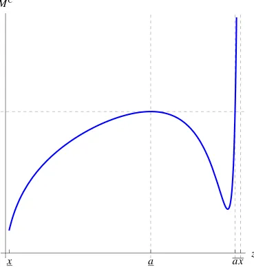
M

Figure 8: MC, the maximand in the C-auxiliary problem. The sign of dMC(z)/dz coin-cides with the sign ofΦ(z,z, ˆc).

suppressed, motivated by the observation that the maximizer in (26) depends onx1 only

through the restriction z _∈ [θ,x1]. To understand the solution of maxz∈[θ,x1]M

C_{(z), it}

is instructive to study the shape of MC on [x, ¯x]. This shape is described by the sign of dMC(z)/dz, which, by differentiation, can be verified to coincide with the sign of

Φ(z,z, ˆc). Figure8illustratesMC.

Note thatΦ(x,x, ˆc) = Φ(x¯, ¯x, ˆc) = 1 (by direct substitution) and thatΦ(z,z, ˆc)is at first

decreasing in zand then increasing in z(by Lemma B.2 in AppendixB) and is uniquely

that, by the definition ofc1in (17) and by LemmaB.1, minzΦ(z,z,c1) = 0. BecauseΦis

strictly increasing in ˆc, ˆc <c1and minzΦ(z,z,c1) =0 imply Φ(z,z, ˆc) <0.

To summarize,Φ(z,z, ˆc)—and hence also dMC(z)/dz—first switches the sign from the positive to the negative and then from the negative to the positive. This

positive-negative-positive sign pattern implies that MC is wave-shaped, with local maxima ata, defined in (28), and ¯x, and with local minima at xand somewhere between aand ¯x. Moreover, by

LemmaB.4of AppendixB, ¯xis the unique global maximum, and soMC(x¯) >MC(a). Coupled with MC(x¯) > MC(a), the wave shape of MC implies the existence of a unique

¯

a ∈ (a, ¯x) such that MC(a¯) = MC(a). Condition MC(a¯) = MC(a) can be simplified to express ¯aequivalently (but still implicitly) by (29).

The derived properties ofMChave the following implications for the program inC(x1)≡

maxz∈[x,x1]M

C_{(z). When x}

1 ∈/ (a, ¯a), MC is maximized on [θ,x1] at x1, and soC(x1) =

V(x1,x1); D1learns. When x1 ∈ (a, ¯a), MC is uniquely maximized on[θ,x1]ata, and so

C(x1) > V(x1,x1); both divisions learn until either division observes the good news or

until both types fall toa, whereupon D1learns.

To characterize the set_Ain Figure7, we formulate theA-auxiliary problemon the set

{x∈ (a∗,a]×[0, 1] | x2 ≥x1}.

In this problem, the choice is when to stop asking D2 to learn and instead adopt the

strategy described in Lemma3, which begins with D1learning. The value of this stopping

problem is, for anyx_{∈ V}ˆ,

A(x)_≡ max z∈[x1,x2]

    

   

1₋(1₋V(x1,z))

1₋x2

1−z −cˆ(1−x2) [ϕ(x2)−ϕ(z)]

| {z }

≡MA_(z;x 1)

    

   

, (31)

anal-ogous to those used in the construction ofVandCabove.

Lemma5characterizes a solution to the A-auxiliary problem in terms of the type

sub-set

A ≡ {x∈ (a∗,a]×[0, 1]| x2 ∈ (d(x1),u(x1))}, (32)

where

a∗ _≡inf_{x1 ∈ [0, 1] | ∃x2∈ [x1, 1] s.t. Φ(x, ˆc) =0}, (33)

d(x1) ≡inf{z∈ [x1, 1]| Φ(x1,z, ˆc) ≤0}, x1 ∈ (a∗, ¯a), (34)

and, lettingb−1denote the inverse function ofb,

u(x1) ≡sup

  

 

z_∈ hx1,b−1(x1)

i

|

1−V(x1,d(x1))

1−d(x1) −cˆϕ(d(x1))

= 1−V(x1,z)

1−z −cˆϕ(z)

  

 

, x1 ∈ (a∗, ¯a). (35)

The origin of the objects entering the definition ofAis revealed in the lemma’s proof.

Lemma 5. Normalize x2 ≥ x1. The value of the A-auxiliary problem in (31) satisfies A(x) =

V(x)if x _∈ (a∗,a]×[0, 1]\A,and satisfies

A(x) =1−[1−V(x1,d(x1))]

1−x2

1₋d(x1) −

ˆ

c(1−x2) [ϕ(x2)−ϕ(d(x1))] (36)

if x ∈ A. The policy that achieves A has D1 learn as in Lemma3if x ∈ (a∗,a]×[0, 1]\Aand

has D2learn if x ∈ A.

Proof. Recall that the maximand in (31) is denoted by MA(z;x1). By differentiating, the

sign of dMA(z;x1)/dz coincides with the sign ofΦ(x1,z, ˆc). Hence, the argument

anal-ogous to the argument in the proof of Lemma4applies, except now, in Φ(x1,z, ˆc), only

one argument,z, varies.

x

d

H

x

L

u

H

x

L

x

z

M

Figure 9: MA, the maximand in the A-auxiliary problem. The sign of dMA(z;x1)/dz

coincides with the sign ofΦ(x1,z, ˆc).

of z, as depicted in Figure 9. By inspection of MA, for a given x1, a local maximum of

MA(z;x1)is given by (34).

Coupled with MA b−1(x1);x1

> MA(d(x1);x1) (by Lemma B.5 of Appendix B), the

wave shape ofMAimplies the existence of a uniqueu(x1) ∈ m(x1),b−1(x1)

such that

MA(u(x1);x1) = MA(d(x1);x1). Condition MA(u(x1);x1) = MA(d(x1);x1) can be

simplified to expressu(x1)equivalently (but still implicitly) as in (35).9

The derived properties ofMAhave the following implications for the program inA(x)≡

9_{As defined in (35),usatisfiesA(x1,u(x}

maxz∈[x1,x2]M

A_(z;x

1). When x2 ∈/ (d(x1),u(x1)), MA(·;x1)is maximized on [x1,x2]at

x2, and so A(x) = V(x). When x2 ∈ (d(x1),u(x1)), MA(·;x1)is uniquely maximized

on[x1,x2]atd(x1), and soA(x) >V(x).

To characterizeB, the remaining set in Figure7, we formulate a degenerate auxiliary

problem, theB-auxiliary problem. The problem is defined on the set

B ≡ {x_∈ (a, ¯a)_×[0, 1] _| x2 ∈ (x1,w(x1))}, (37)

whereais defined in (28), ¯ais defined in (29), and

w(x1) ≡inf

n

z _∈ hx1,b−1(x1)

i

| V(x1,z) = B(x1,z)

o

, x1∈ (a, ¯a). (38)

The problem consists in having D2 learn until it observes the good news or until its

re-vised type drops down to D1’s typex1(the “choice” of this thresholdx1is the degenerate

decision), whereupon both divisions learn as prescribed by the C-auxiliary problem. This

policy’s value is

B(x)≡1−(1−C(x1))

1−x2

1₋x1 −

ˆ

c(1−x2) [ϕ(x2)−ϕ(x1)]. (39)

The function B is constructed using the arguments analogous to those used in the

con-struction ofV,C, and Aabove.

We can now assemble the pieces.

Lemma 6. Suppose that learning is cheap, orcˆ<c1. The conjectured value function

F(x) = 1_{x∈A}A(x) +1_{x∈B}B(x) +1_{x∈C}C(x) +1_{x∈V}V(x) +1_{x∈I}x2

g-solves HJBQVI and satisfies the boundary condition.

1. Suppose that x ∈ I, so that F(x) = x2. HJBQVI holds by Step 1 in the proof of

Lemma3.

2. Suppose that x _{∈ V}, so that F(x) = V(x). HJBQVI follows from the argument in

Step2in the proof of Lemma 3with one modification. Part2cof that step requires

the inequalityΦ(x, ˆc) _≥0. To show this inequality here, note thatΦ(x, ˆc) <0 _⇐⇒

x _{∈ F}, by the definition of the failure set _F in (23). Because _{F ⊂ A ∪ B ∪ C} (by

Lemmas B.5 and B.6) and V ∩(A ∪ B ∪ C) = ∅ (by the definition of V in (24)),

x ∈ V impliesx ∈ F/ . As a result,Φ(x, ˆc) ≥0 for allx ∈ V, as desired.

3. Suppose thatx _{∈ C}, so that F(x) = C(x2) and ∂F(x)/∂xi = (1/2)∂C(xi)/∂xi.10 HJBQVI in (5) will be verified component by component of the min function:

min

ˆ

c+ x2(1−x2)

2

∂C(x2)

∂x2 −x2(1−C(x2)),C(x2)−x2

=0.

(a) The inequality C(x2) ≥ x2 follows by “revealed preference.” By construction

of the C-auxiliary problem, C(x2,x2) ≥ V(x2,x2). By construction of the

V-auxiliary problem,V(x2,x2) ≥x2. Therefore,C(x2) ≥x2.

(b) To show

ˆ

c+ x2(1−x2)

2

∂C(x2)

∂x2 −

x2(1−C(x2)) =0, (40)

differentiateCin (30) to obtain

∂C(x2)

∂x2

= 2

1−x2

1−C(x2)−

ˆ

c x2

. (41)

Substitution of the above display and ofCinto (40) verifies the equality.

4. Suppose x ∈ A ∪ B. If x ∈ A, then F(x) = A(x). If x ∈ B, then F(x) = B(x).

10_{Note the notational convention according to which∂F(x)/∂x}

i 6= ∂C(xi)/∂xi. The rationale is that ∂F(x)/∂xi is the change in the conjectured value function in response to a marginal change in a single

type, whereas∂C(xi)/∂xiis the change in the conjectured value function in response to identical marginal

HJBQVI is verified component by component of the min function:

min   

 

ˆ

c+x1(1−x1) ∂F_∂x(x₁) −x1(1−F(x)),

ˆ

c+x2(1−x2)∂F_∂x(x₂) −x2(1−F(x)),F(x)−x2

  

 

=0.

(a) To verify

ˆ

c+x2(1−x2)∂

F(x)

∂x2 −x2(1−F(x)) =0, (42)

replaceFand∂F/∂x2in the display above byAand∂A/∂x2ifx∈ A, and byB

and∂B/∂x2if x∈ B. The function∂A/∂x2is obtained by differentiating (36):

∂A(x) ∂x2

= 1−V(x1,d(x1))

1₋d(x1)

+cˆ(ϕ(x2)−ϕ(d(x1)))− cˆ

x2(1−x2)

.

The function∂B/∂x2is obtained by differentiating (39):

∂B(x) ∂x2

= 1−C(x1)

1₋x1

+cˆ(ϕ(x2)−ϕ(x1))−

ˆ

c x2(1−x2)

.

(b) To showF(x) _≥ x2, it suffices to show F(x) ≥V(x)and, in order to conclude

thatV(x) _≥ x2by construction of the V-auxiliary problem, to show x ∈ A ∪

B =⇒ x∈ _Vˆ_{. Hence, it will be shown that (i)A(x) ≥V(x)andB(x) ≥V(x),}

and (ii)A ⊆ _Vˆ _{and B ⊆V}ˆ_.

i. Whenx ∈ A, A(x)≥V(x)follows “by revealed preference,” by

construc-tion of the A-auxiliary problem.

When x _{∈ B}, showingB(x) _≥ V(x) is mildly more involved, but is also

essentially a revealed-preference argument, applied twice. In particular,

extend the A-auxiliary problem (originally defined on _A) onto the set _B.

Using the same arguments as in Lemma 5, this problem’s solution can be

verified to imply that, whenever x ∈ B, D2 learns until either he observes

prescription of the V-auxiliary problem is followed, delivering the

contin-uation valueV(x1,x1). So, by revealed preference, A(x) ≥V(x).

OnB, the B-auxiliary problem has the same threshold as the extended

A-auxiliary problem, but once this threshold has been reached, delivers a

higher continuation value, C(x1), with C(x1) ≥ V(x1,x1) by “revealed

preference” in the C-auxiliary problem. So, B(x) _≥ A(x), which,

com-bined with A(x) _≥V(x), givesB(x) _≥V(x), as desired.

ii. The inclusionA ⊆ _Vˆ _{follows because LemmaB.5 shows that x1 ∈ (a}∗_,a)

implies u(x1) <b−1(x1). That is,u(x1), the upper boundary of setA, on

which the A-auxiliary problem is defined, lies strictly below b−1(x1), the

upper boundary of set ˆ_V.

The inclusion _{B ⊆ V}ˆ follows because Lemma B.6 shows that x1 ∈ (a, ¯a)

implies w(x1)<b−1(x1). That is,w(x1), the upper boundary of setB, on

which the B-auxiliary problem is defined, lies strictly below b−1(x1), the

upper boundary of set ˆV.

(c) It will be shown that

ˆ

c+x1(1−x1)

∂F(x) ∂x1 −

x1(1−F(x))≥0. (43)

Ifx∈ A, apply the Envelope Theorem toAin (36) to obtain

∂A(x) ∂x1

= ∂V(x1,d(x1))

∂x1

1₋x2

1−d(x1)

.

inequality (43) and dividing by ˆcyields the equivalent tentative inequality

1 ≥x1(1−x2) (ϕ(x2)−ϕ(d(x1)))

+ x1(1−x2)

(1₋d(x1))cˆ

1−V(x1,d(x1))−(1−x1) ∂V(x1,d(x1))

∂x1

,

which further simplifies by substitutingV and ∂V/∂x1 using (19) and by

di-viding both sides by 1₋x2:

1

1−x2 ≥x1(ϕ(x2)−ϕ(d(x1))) +

1 1−d(x1)

. (44)

Ifx_{∈ B}, differentiateBin (39) and use the expression for∂C(x1)/∂x1to obtain

∂B(x1,x2)

∂x1

= 1−x2

(1−x1)2

1−C(x1)−

ˆ

c x1

.

Substituting the above display and the definition ofBin (39) into the tentative

inequality (43) leads, once again, to the tentative inequality (44).

If x2 = d(x1), the inequality (44) holds trivially, as equality. To show that

the inequality holds also forx2 > d(x1), it suffices to show that its left-hand

side increases inx2 faster than its right-hand side. Indeed, the left-hand side’s

derivative, which is 1/(1−x2)2, is larger than the right-hand side’s derivative,

which is

x1ϕ0(x2) =

x1

x2(1−x2)2

,

byx1< x2. Thus, the tentative inequality (44) is definitive, as desired.

3.5

Synthesis

To summarize, theconjectured value functionis

F(x) =

            

           

x2 ifc2 ≤cˆ

1_{x∈V}V(x) +1_{x∈I}x2 ifc1 ≤cˆ<c2

1_{x∈A}A(x) +1_{x∈B}B(x)

+1_{x∈C}C(x) +1_{x∈V}V(x) +1_{x∈I}x2

if ˆc <c1,

(45)

where A, B,C, andV are defined, respectively, in (36), (39), (30), and (16).

The underlying conjectured optimal policy can be read off Figure 2 when c2 ≤ cˆ,

Figure3whenc1 ≤cˆ<c2, and Figure5when ˆc <c1.

4

Verification of the Conjectured Value Function

Theorem 1. The conjectured value function F in (45) is the sought value function; that is,φ=F.

By implication, the conjectured optimal policy is indeed optimal.

The theorem’s proof builds on several intermediate results and is distilled toward the

end of the section.

4.1

The Big Picture

Continuous-time modelling enables us to compute explicitly HQ’s value function and

derive the implied optimal policy. In addition, the statements of the results are not

con-taminated by provisos stemming from the indivisibility of information increments, which

would be inherent in any discrete-time formulation. The cost of the continuous-time

ap-proach is the unfamiliar mathematics required to rigorously justify the results. In

number of technical conditions are also invoked. Therefore, before delving into the formal

analysis, we informally outline the main ideas and relate continuous-time optimization

to its familiar discrete-time counterpart.

Consider the dynamic programming principle (DPP). DPP says that HQ’s value today

equals HQ’s expected continuation value at an arbitrary future stopping time plus the

flow payoffs enjoyed until that time. These intervening flow payoffs and the eventual

continuation value depend on the intervening controls, which are chosen to maximize

HQ’s value today. This statement of DPP is the same in both continuous and discrete

time and relies on the same backward-induction argument. The argument requires either

a finite horizon or discounting. We impose neither. However, without loss of generality,

we could have imposed a finite horizon. Indeed, if learning is protracted, eventually,

beliefs become so precise that further learning cannot possibly justify its costs. So DPP

holds in our setting.

One can show that DPP holds if and only if the DPP equation holds for the

small-est possible positive stopping time. In a discrete model, this smallsmall-est time is one period,

and the corresponding DPP equation is known as the Bellman equation. In a continuous

model, the smallest time is operationalized by taking limits, thereby obtaining a

differen-tial counterpart of the Bellman equation, known as the HJBQVI equation. Taking limits

is delicate, however, because limits may not exist, even under natural “technical”

condi-tions. That is, the value function need not be differentiable; it may have “kinks.” Kinks

are not an issue in discrete time, because the Bellman equation is not a differential

equa-tion.

In continuous time, kinks cannot be neglected. A candidate value function that solves

HJBQVI at all points of differentiability but with its kinks unrestricted may fail to be the

sought value function. That is, extraneous generalized solutions of HJBQVI are possible.

Enter viscosity solution, which uses HJBQVI to discipline the candidate value function

In our maximization problem, viscosity solution restricts upward kinks, but not

down-ward kinks.11 It is somewhat of a folk wisdom that, in maximization problems, value

functions abhor upward kinks. For instance, that, in a static problem, under natural

con-ditions, the value function admits no upward kinks can be seen graphically by taking the

upper envelope of the reward functions for various values of the control while varying the

state. Clausen and Strub (2012) show how upward kinks can be ruled out in a dynamic

problem (not related to ours).12 HJBQVI’s viscosity solution strengthens generalized

so-lution by imposing the requisite optimality restrictions on the kinks. A characterization

theorem obtains; the sought value function, and only this function, is the viscosity

solu-tion of HJBQVI.

The conjectured value function Fin (45) has no upward kinks at all, as will be shown.

(The downward kinks are where regions A and B border V in Figure 7 and on the

45-degree line except within the heart-shaped region in Figures 4 and 7.) So the viscosity

conditions on the kinks hold automatically. All that remains to verify is that HJBQVI

holds at all points of differentiability, which we have already done. Thus, the conjectured

value function is the viscosity solution of HJBQVI and hence is the sought value function.

To summarize, the conditions that viscosity solution imposes on kinks are substantive,

not technical. The economic content of these conditions is not peculiar to the

continuous-time model. In the discrete model, the same content is already embedded into the Bellman

equation, which is comprehensive because it is not restricted to the value function’s points

of differentiability. Just as, in discrete time, the value function is the unique solution

of the Bellman equation, in continuous time, the value function is the unique viscosity

solution of HJBQVI. This viscosity characterization of the value function is the essence of

the verification procedure, justified and performed in the remainder of this section.