ARABIC NAMED ENTITY RECOGNITION IN CRIME DOCUMENTS

ISSN: 1992-8645 www.jatit.org E-ISSN: 1817-3195

SMOOTH SUPPORT VECTOR REGRESSION BASED ON

MODIFICATION SPLINE INTERPOLATION

1 _{BIN REN,} 1 _{HUIJIE LIU,} 1 _{LEI YANG,} 2 _{LIANGLUN CHENG}

1 _{School of Electronic Engineering, Dongguan University of Technology, Dongguan, 523808, China}

2

School of Automation, Guangdong University of Technology, Guangzhou,510006, China

ABSTRACT

Regression analysis is often formulated as an optimization problem with squared loss functions. Facing the challenge of the selection of the proper function class with polynomial smooth techniques applied to Support Vector Regression models, this study takes three interplation points spline interpolation technology and modification interpolation value to generate a new polynomial smooth function _|x|2

ε in ε-insensitive support vector regression. The experimental analysis shows that 2

M

S _ε-function is better than _p2

ε-function and _S2

ε-function in properties, and the approximation accuracy of the proposed smooth function is three order of higher than that of classical _p2

ε-function.

Keywords: Support Vector Regression, ε-insensitive Loss Function, Smooth Polynomial Function,

Modification Interpolation

1. INTRODUCTION

Smooth function has been widely studied in numerical modeling[1-6], which, especially in the interest of the authors, has been successfully applied for classification of and regression model fittings in image processed and pattern recognition[2, 3, 7, 8]. Applying smooth function to regression models means to deal with square unsmoothed issue in ε-insensitive loss function while fitting the regression models [8]. According to the basic concept on how to solve classification problem, Lee et al, used _p2

ε -function as to smoothly approach the target function, and brought forward the ε-insensitive support vector regression model (ε-SSVR) in 2005 [8]. Their results show that the effect of ε-SSVR is better than both LIBSVM[9] and _SVMlight_{[10] in both regression}

property and efficiency.

It is, however, still an open and challenging issue to find a better smooth function [1,2,5,7,9]. Accordingly this paper is motive to present a study on using three interpolation points Cubic Spline Interpolation polynomial and modification interpolation value to improve this kind of smooth function in fitting support vector regression model. The proposed 2

M

S _ε -function is better than _p2 ε -function and _S2

ε -function in property, and the approximation accuracy of the proposed smooth function is three order of higher than that of

classical p_ε2-function and one order of higher than

that of classical p_ε2 -function S_ε2 -function. The simulation case study shows that it improves the regression effect.

This paper is organized as follows: section 2 introduces regression problems and difficulties. section 3 introduces ε-insensitive loss function and

support vector regression .In Section 4, we first introduce the principle and derive formula of Cubic Spline Interpolation polynomial, then use Modification Spline Interpolation polynomial to smooth single variable positive function, and we define _|x|2

ε’s polynomial approximation function 2 _{( , )}

M

S _ε x k . In Section 5, we analyze the performance of polynomial smooth approximation function 2 _{( , )}

M

S _ε x k . It is the 1st-order smooth

function, and the approximation accuracy is 0.0081/k. Section 6, we run two numerical simulation experiments by using data sets from artificial database and UCI database to verify the validity of the model. Finally, we make a conclusion and foresee the future work in section 7.

2. REGRESSIONBASEDDATAFITTING

First, we discuss the simplest regression problem in 2-dimensional space: Let’s suppose all values

1

x , x₂ , ... , x_m from 1 to m, each x is _i

ISSN: 1992-8645 www.jatit.org E-ISSN: 1817-3195 purpose is using the designated data set to generate

interdependent functiony= f x( ). We usually use this way to solve the problem as below: first, to restrict the function y= f x( ) in a simple function

class in advance, then searching for f x that can ( ) meet the following conditions in the function class as mush as possible:

( ) , 1, 2, ,

i i

y = f x i= L m (1)

In order to easy to deal with, we always use linear regression way, i. e., restricting f x to be ( )

linear functionf x( )=wx b+ . Then search for f (x) which can meet the equation (1).

2 2

(y_i− f x( ))_i =(y_i−wx_i−b) (2)

Equation (2) is often used to measure the deviation degree between y= f x( )=wx+b and

( )

i i

y = f x .The smaller value is, the less error is and higher efficient it is. So this process can be translated into the following optimized formula. So that we can define w and b in the function f x( )=wx+b :

2 ,

1

min ( )

m

i i

w b i

y wx b

=

− −

∑

(3)

Obviously, the regressive formula and solution above can be extended to a normal situation.

First, extending data class (1) to data set S:

1 1

{( , ), , ( , )} n

m m

S = x y _L x y ⊆R ×R (4)

Secondly, the function class which restrict the function y=f (x) (1) above also can be extended to be a real function setF. Generally, there is not only criterion to measure the deviation of regression function y= f x( ) from yi = f x( )i . We call

equation (3) above as quadratic loss function. Of course, other loss function also can be used. If we name loss function as c x y f( , , ) . The optimized formula (3) will become minimization formula with empirical risk.

1

min ( , , ( ))

m

i i i

f F i

c x y f x

∈

∑

₌ (5)

Thus, the interdependent functiony= f x( ) can be obtained, i. e., regression function.

When solving the optimized formula(5), the first issue is how to choose the function class set F. For the designated normal training data set S (4), we can not restrict F to be too small function class,

such as linear functions will produce large regression error in a model in nature of nonlinearity. On the other hand, F cannot be too large otherwise the regression function will be meaningless. For example, we will obtain the following equation based on data set S (4) when F is the whole real function set.

, ( ) {

0,

i i

i

y x x

f x

x x

= =

≠ i=1, 2L, .m (6)

Obviously, the regression function is too illogical. Accordingly the key point is how to choose the function class set F, neither too simple nor too complicated. Furthermore, it becomes difficult to choose the right one for the regression function.

3.

S

UPPORT

V

ECTOR

R

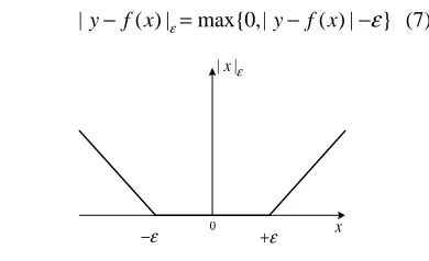
EGRESSION

For better analysis, we define the ε-insensitive

loss function of independent variable X as x_ε ,

|x|_ε=max{0,|x|−ε} , as shown in Figure 1. Definition the square of ε-insensitive loss function

as _|x|2

ε , and the positive function x+ as (x₊)_i =max{0, }x_i .

Data set {( ,_{1 1}), , ( , )} n

m m

S= x y _L x y ⊆R ×R ,

define matrix A=[x x₁, _2,⋅⋅⋅x_m], x_i is n dimensional

vector, each x_iis corresponding with an observed

value y_i , obviously _A∈Rm n× _{, that it is}

{( _i, _i) | _i n, _i , 1, , }.

S= A y A ∈R y ∈R for i= L m

The purpose is using the designated data set S to generate a regression function f x( ) , let f x( ) predict y more accurately according to the new input of x. The standard we use is ε-insensitive loss

function:

|y−f x( ) |_ε=max{0,|y− f x( ) |−ε} (7)

x | |x_ε

ε

[image:2.612.326.521.555.674.2]

− +ε

Figure 1: Ε-Insensitive Loss Function x_ε

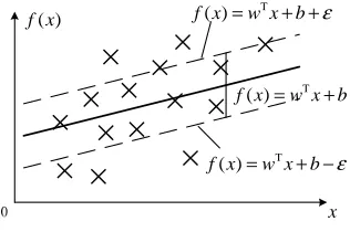
For linear regression case,f x( )=w xT +b, where

n

ISSN: 1992-8645 www.jatit.org E-ISSN: 1817-3195 indeterminate constant. ε-insensitive linear

regression function is shown in Figure 2, we select two hyperplanes of the margin in a way and we call the distance between the two hyperplanes is ε zone.

Only by there are no training points falling into the margin, we can have loss, and the loss is

|y− f x( ) |-ε.

x ( )

f x

×

×

×

×

× ×

×

×

×

×

×

×

×

×

×

T ( )

f x =w x b+ −ε

T ( )

f x =w x b+

T ( )

[image:3.612.104.262.186.291.2]

f x =w x b+ +ε

Figure 2: Ε-Insensitive Linear Regression Function

For nonlinear regression case f x( )=ωϕ( )x +b, where ( )ϕ ⋅ : nonlinear function. In theory, we can change it into linear regression ones to settle it according to kernel technique.

Standard regression problem is to solve the following minimum problem [11]:

* 1 *

2

1

*

*

min ( , , , ) ( )

. . ( )

( )

0, 0, 1, 2, ,

n T

i i i

i i i

i i i

i i

Q b C

s t y x b

x b y

i n

ω ξ ξ ω ω ξ ξ

ω ϕ ε ξ ω ϕ ε ξ ξ ξ

=



= + +

 

 _{− ⋅ − ≤ +}



 _{⋅ + − ≤ +}



 _{≥ ≥ = ⋅⋅⋅}



∑

(8)

Where

1 2

( , , , _n) ,T

ξ = ξ ξ ⋅⋅⋅ξ * * * *

1 2

( , , , _n)T

ξ = ξ ξ ⋅⋅⋅ξ , ε( 0)

is the maximum deviation allowed during the training and C(>0) represents the associated penalty for excess deviation during the training. The slack variables ξ_iandξ_i*, correspond to the size of this excess deviation for positive and negative deviations respectively. The first term,ω ωT is the regularized parameter; thus, it controls the function

capacity; the second term * 1

( )

n

i i i

ξ ξ

= +

∑

, is the

empirical error measured by the ε-insensitive loss

function.

The computation of Standard support vector regression is more complicated, because when solving the Optimization problem, you need to solve quadratic programming, especially when the training sample number is increased. The solution

will face curse of dimensionality, in result that we can’t train it. Suykens J.A.K [11] proposes least squares method-support vector machines (LS-SVM) to make the problem comes down to linear equations, and solving linear equations is easier and faster than the quadratic programming. Standard regression problem is to solve the following problem:

2 1

2

1

min ( , )

2

. . ( ) , 1, 2, ,

n T

i i

i i i

C Q

s t y x b i n

ω ξ ω ω ξ

ω ϕ ξ

= 

= +

 

 _{= ⋅ + = ⋅⋅⋅}



∑

(9)

In addition, Lee et al adds the parameter 2

1

2b into the objective function to induce strong convexity and to guarantee that the problem has a unique global optimal solution. The regression issue can be expressed by below unconstrained optimized issue formula [9]:

1

2 2

( , ) ₁

1

min ( ) | | .

2 2

n

m T

i i

w b R _i

C

w w b A w b y _ε

+

∈ + +

∑

₌ + − (10)

Obviously, the _|x|2

ε in formula (10) is not derivative, so this target function is not derivative.

4. POLYNOMIALSMOOTH

APPROXIMATIONFUNCTION

Cubic spline function may generate smooth interpolation curve by combining the discontinuous cubes and the second derivative is continuous at the joint point, namely sampling point.

4.1 Mathematical Description

Assumption a set of nodes

0 1 ... n

a≤x < < <x x ≤b at[ , ]a b , if the function s(x) meet below term[11],

(1) s x( )∈C a b2[ , ];

(2) s x( ) is cubic polynomial at every region

1

[ ,x x_{i i+}] (i=0,1,...,n−1).

If s(x) also meets the following spline term at node,

(3)S x( )_i = f i_i, =0,1,...n .

Then s x( ) is called cubic spline interpolation

function, the second derivative of s x( ) at [ , ]a b is continuous.

ISSN: 1992-8645 www.jatit.org E-ISSN: 1817-3195

x+, at the end point a=x0,b=xn of region [a,b],

using following boundary conditions: ' '

0 0

( )

S x = f ,

' '

( _n) _n

S x = f , at region[ ,x xi i+1], the formula of cubic spline function is

3 3 2

1 1

1

( ) ( )

( ) ( )

6 6 6

i i i i i

i i i

i i i

x x x x M h x x

S x M M f

h h h

+ + + − − − = + + − 2 1 1 ( ) 6

i i i

i

i

M h x x

f

h

+ +

−

+ − (i=0,1,⋅⋅⋅ −,n 1) (11)

To solve M we can write it in matrix form as _j

following:

0 0

1

1 1 1

1 1 1 2 1 2 ... ... ... ... ... 2 1 2 n n n n d M d M d M d Mn µ λ

λ− − −                        ₌                         (12)

Where: d₀ =6f x x x

[

₀, ,_{1 0}

]

(13)

[

1 1

]

6 , ,

i i i i

d = f x− x x+ (14)

[

1

]

6 , ,

n n n n

d = f x x− x (15)

1 1 i i i i h h h µ − − =

+ (16)

1 1 i i i i i h h h λ µ − = − =

+ (17)

1

i i i

h = −x x₋ (18)

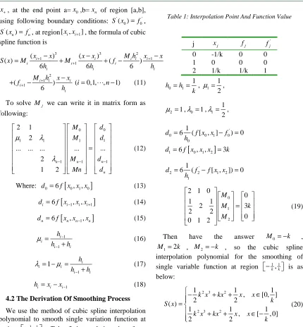
4.2 The Derivation Of Smoothing Process

We use the method of cubic spline interpolation polynomial to smooth single variation function at region 1_,1

k k

−

 

 . Take 3 interpolation data from positive function x+ at region x<0 x=0 and x>0m ,

point 1

j k

x = − , xj+1=0 and xj+2 =1k (k>0),

corresponding f_j =0,fj+1 =0, 1 2

j k

f ₊ = .

Using cubic spline interpolation polynomial to smooth positive function x₊ at region 1_,1

k k

−

 

[image:4.612.92.522.87.551.2]

  , table 1 is interpolation point, corresponding function and the first derivative value.

Table 1: Interpolation Point And Function Value

j x j f j

' j f 0 1 2 -1/k 0 1/k 0 0 1/k 0 0 1 0 1 1 h h k

= = , ₁ 1

2

µ = ,

2 1

µ = ,λ₀ =1, ₁ 1 2

λ = ,

'

0 0 1 0

0 1

6 ( [ , ] ) 0

d f x x f

h

= − =

[

]

1 6 0, 1, 2 3

d = f x x x = k

'

2 2 1 2

1 1

6 ( [ , ]) 0

d f f x x

h

= − =

0

1

2

2 1 0

0

1 1

2 3

2 2

0 0 1 2

M M k M               ₌                  (19)

Then have the answer M0 = −k ,

1 2

M = k , M2 = −k , so the cubic spline interpolation polynomial for the smoothing of single variable function at region 1_,1

k k

−

 

  is as below:

2 3 2

2 3 2

1 1 1

, [0, ]

2 2

( )

1 1 1

, [ , 0]

2 2

k x kx x x

k S x

k x kx x x

k  − + + ∈  =  _{+ + ∈ −}  (20) ( )

S x ≤x₊, in x= ±1 / 3k, the difference value is

the largest, max(x₊−S x( ))=2 / 27k . In order to

make S x greater than x( ) +, the S x as a whole ( ) moves up to 2 / 27k [12].

[image:4.612.298.521.123.553.2]

ISSN: 1992-8645 www.jatit.org E-ISSN: 1817-3195

2 3 2

2 3 2

1 3

1 1 2 1

, 0

2 2 27 3

( , )

1 1 2 1

, 0

2 2 27 3

1

0 0

3

M

x x

k

k x kx x x

k k

S x k

k x kx x x

k k

x k

k



≥

 

_{− + + + ≤ <}



=

 _{+ + + − < <}

 

 _{≤ − >}



(21)

4.3 The polynomial approaching function S_M2_ε of

2

x_ε

Define S_M2_ε( , )x k is the square of polynomial

approaching function S_Mε( , )x k for ε-insensitive

loss function x_ε , from formula (21) we have

following conclusion:

2 1

3

2 3 2 2 1

3

2 3 2 2 1

3

2 1 1

3 3

2 3 2 2 1

3

2 3 2

( ) ,

1 1 2

( ( ) ( ) ( ) ) ,

2 2 27

1 1 2

( ( ) ( ) ( ) ) ,

2 2 27

( , ) 0 ,

1 1 2

( ( ) ( ) ( ) ) ,

2 2 27

1 1

( ( ) ( ) (

2 2

k

k

k

M k k

k

x x

k x k x x x

k

k x k x x x

k

S x k x

k x k x x x

k

k x k x x

ε

ε ε

ε ε ε ε ε

ε ε ε ε ε

ε ε

ε ε ε ε ε

ε ε

− ≥ +

− − + − + − + < < +

− + − + − + − + < <

= − ≤ ≤ − +

− + + + − + + − < < −

+ + + − 2 1

3

2 1

2

) ) ,

27

( ) ,

k

k

x k

x x

ε ε ε

ε ε

            

+ + − − < < − 



 _{− − ≤ − −}



(22)

5. PROPERTYANALYSIS

Lemma 1[8] _p2

ε-function

2_{( , ) ( ( , ))}2 _{( ( , ))}2

p x k_ε = p x−ε k + p − −x ε k ,

where _{p x k}( , ) _x 1 ln(1 _ekx)

k

−

= + + ,k>0 , e is

the base of natural logarithm, it has the following properties:

(1) p_ε2-function is any-order smooth w.r.t. x;;

(2) p x k_ε2( , ) |≥ x|_ε2;

(3) Forx∈Rand|x <| ρ ε+ :

2_{( , ) | |}2 ₂₍log 2₎2 2 _{log 2}

p x k x

k k

ε − ε≤ + ρ .

Lemma 2[13] _S2

ε-function

2 1

2 2 1 1

2 1 1

2 2 1 1

2 1

( ) ,

1 1 1

( ( ) ( ) ) ,

4 2 4

( , ) 0 ,

1 1 1

( ( ) ( ) ) ,

4 2 4

( ) ,

k

k k

k k

k k

k

x x

k x x x

k

S x k x

k x x x

k

x x

ε

ε ε

ε ε ε ε

ε ε

ε ε ε ε

ε ε

 _{− ≥ +}



 _{− + − + − + < < +}

 

= − ≤ ≤ − +



 _{+ − + + − − < < −}

 

− − ≤ − −



(23)

has the following properties:

(1) S_ε2 is 1st-order smooth w.r.t. x. That is, at interpolation points,

2 1

2 1 ( (_k ), )

S k

k

ε ± +ε = Sε2( (± − +1k ε), )k =0

2 1 2

( ( ), )

S k

k k

ε ε

∇ ± + = S2( ( 1 ), )k 0;

k

ε ε

∇ ± − + =

ISSN: 1992-8645 www.jatit.org E-ISSN: 1817-3195

(3) 2( , ) | |2 1₂ 11

S x k x

k

ε − ε≤

Theorem 1 S_M2_ε is defined in(16), we have:

(1) S_M2_ε is 1st-order smooth w.r.t. x. That is, at interpolation points,

2 1

3 2

1

( ( ), )

9

M k

S k

k

ε ± +ε = (24)

2

2 4 ( , )

729

M

S k

k

ε ±ε = (25)

2 1

3

( ( ), ) 0

M k

S _ε ± − +ε k = (26)

2 _{( (}1 _{), )} 2

3 3

M

S k

k k

ε ε

∇ ± + = (27)

2 _{( , )} 2

27

M

S k

k

ε ε

∇ ± = (28)

2 _{( (} 1 _{), ) 0}

3

M

S k

k

ε ε

∇ ± − + = (29)

(2) S_M2_ε( , ) |x k ≥ x|2_ε (30)

(3) 2 ( , ) | |2 1 ₂ 124

M

S x k x

k

ε − ε≤ (31)

Proof:

(1) According to the definition, we can directly prove it.

(2) Verify S_M2_ε( , ) |x k ≥ x|_ε2

For 1 k

x≥ +ε , 1

k

x≤ − −ε and − ≤ ≤ε x ε , Conclusion is obviously correct.

For 1

k

x

ε< < +ε, define:

2 2

( ) ( , ) | |

g x =S_ε x k − x_ε , then we have

2 3 2

1 1

( ) ( ( ) ( ) ( )

2 2

g x = − k x−ε +k x−ε + x−ε

2 2 2 3

2 1

) ( ) ( ( )

27k x ε 2k x ε

+ − − = − −

2 3 2

( ) ( ) )

2 27

k x x

k

ε ε

+ − + − + •

2 3 2

1 1 2

( ( ) ( ) ( ) )

2k x ε k x ε 2 x ε 27k

− − + − − − +

Define:

2 3 2

1

1 3 2

( ) ( ) ( ) ( )

2 2 27

h x k x k x x

k

ε ε ε

= − − + − + − +

2 3 2

2

1 1 2

( ) ( ) ( ) ( )

2 2 27

h x k x k x x

k

ε ε ε

= − − + − − − +

Then we get ₁( ) 4 ₂

729

h

k

ε = , for

1 3k

x

ε< < +ε

2 2

1

3 3

( ) ( ) 2 ( )

2 2

h x k x ε k x ε

∇ = − − + − +

2 2

3

(1 ( ) ) 2 ( ) 0

2 k x ε k x ε

= − − + − > .

So h x1( ) is strictly monotonic increasing at

region 1

3k

x

ε< < +ε . So for 1 3k

x

ε < < +ε ,

1( )

h x > 1 2

4

( ) 0

729

h

k

ε = > , so,h x1( )>0Then we

get 1

2(3k ) 0

h +ε =

For 1

3k

x

ε< < +ε

2 2

2

3 1

( ) ( ) 2 ( )

2 2

h x k x ε k x ε

∇ = − − + − −

1

(1 ( ))(1 3 ( )) 0

2 k x ε k x ε

= − − − − − <

So h x is strictly monotonic decreasing at 2( )

region 1

k

x

ε< < +ε . So for 1 k

x

ε< < +ε ,

2( )

h x > 1

2(k ) 0

h +ε = , so,h x2( )>0.

then S_M2_ε( , ) |x k ≥ x|_ε2 is correct for

1 3k

x

ε< < +ε.

Similarly, for the case of− − < < −3k1 ε x ε, we have S_M2_ε( , ) |x k ≥ x|2_ε.

Hence, S_M2_ε( , ) |x k ≥ x|2_ε

(3) Verify 2 ( , ) | |2 1 ₂ 124

M

S x k x

k

ε − ε≤

For 1

3k

x≥ +ε, 1

3k

x≤ − −εand 1 1

3k− ≤ ≤ − +ε x 3k ε ,

the conclusion is obviously correct.

For− + < <3k1 ε x ε,we have

2 _{( , ) | |}2 2 _{( , )}

M M

S _ε x k − x_ε=S _ε x k ,due to 2 M

S _ε is a strictly monotone increasing function for

1 1

3k ε x 3k ε

ISSN: 1992-8645 www.jatit.org E-ISSN: 1817-3195

2 2

2 2

4 1

( , ) ( , )

729 124

M M

S x k S k

k k

ε ≤ ε ε = < ;For

1 3k

x

ε ε

− < < − ,we have

2 _{( , ) | |}2 2 _{( , )}

M M

S _ε x k − x_ε=S _ε x k ,due to 2 M

S _ε is a strictly monotone decreasing function for

1 1

3k ε x 3k ε

− − < < − ,so

2 2

2 2

4 1

( , ) ( , )

729 124

M M

S x k S k

k k

ε ≤ ε ε = < ; For

1 3k

x

ε< < +ε

2 2

( ) _M ( , ) | |

g x =S _ε x k − x _ε ,we have variable substitution for formula:

2 3 2

1 1

( ) ( ( ) ( ) ( )

2 2

g x = − k x−ε +k x−ε + x−ε

2 2

2

) ( )

27k x ε

+ − − , a=k x( − ∈ε) (0,1) ,then

2 2

3 2

2

1 1 2

( ) ( )

2 2 27

a a

g a a a

k k k k k

= − + + + − has

maximum value point a=0.0751 at region

0<a<1,hence ( ) (0.0751) 1 ₂ 124

g x g

k

≤ < ,therefore,

the conclusion is correct.

Similarly, for the case of ₃1

k ε x ε

− − < < − , we

have ( ) (0.0751) 1 ₂

124

g x g

k

≤ < .

Hence, 2 ( , ) | |2 1 ₂ 124

M

S x k x

k

ε − ε≤ .

6. EXPERIMENTALRESULT

In the case of k=5,ε=0.3, the smooth function approximation comparison chart is as Figure 3, then we can see that, SM2ε -function has higher

approximation accuracy than _p2

ε -function and Sε2 -function with the same K value.

When p_ε2-function and S_ε2-function as smooth

functions, define ρ=1/ k , from Lemma 1 and Lemma 2 we have p x k_ε2( , ) | |− x_ε2≤1.3854 /k2 and

2 2 2

( , ) | | 0.0909 /

S_ε x k − x_ε≤ k , Table 2 list the approximation accuracy of three smooth functions, then we can see that the approximation accuracy of

2 M

S _ε-function is three order of magnitude higher

than that of the p_ε2 -function and one order of

magnitude higher than that of the S_ε2-function at the same K value.

Figure 3: Smooth Function Approximation

Comparison Chart In The Case Of K=5 And Ε=0.3

Table2: Approximation Accuracy Of Smooth Functions

smooth function

2

p_ε- function

2

S_ε- function

2 M

S _ε- function approximation

accuracy

2

1.3854 / k 2

0.0909 / k

2 0.0081 / k

To further verify the property of this smooth function applying to support vector regression, Two simulated experiments were selected to demonstrate the analytical results, which were run at Matlab7.0 on a personal computer with an AMD X4 620 processor and 2GB memory. Based on the first order optimality conditions of unconstrained convex minimization problem, our stopping criterion was satisfied when the 2-norm of gradient of the objective function is less than ₁₀−5_{.For an} observation vector y and the prediction vector ˆy , the 2-norm relative error of two vectors y and

ˆy was defined as follows:

2

2 ˆ

|| ||

|| ||

y y

y

−

(32)

ISSN: 1992-8645 www.jatit.org E-ISSN: 1817-3195 ability. We performed tenfold cross-validation on

each data set and reported the average testing error in our numerical results. To generate a highly nonlinear function, a Gaussian kernel was used for all nonlinear numerical tests defined as below:

2 2

|| ||

( , T) Ai Aj , , 1, 2, 3, ,

i j

K A A =e−µ − i j= L m (33)

The parameters µ and C were determined by a tuning procedure.

First, we selected 101 points evenly from [-1, 1] as the input data of the artificial data sets and the observation was generated from a simple function as follows:

30

sin( )

( ) 0.5 ,

30 x f x

x

π _ρ

π

[image:8.612.326.509.324.398.2]

= ⋅ + (34)

Table 3: Numerical Result For Sin Function

Methods #SVs Train Error(%)

Test Error(%)

CPU (s)

ε-PSSVR

ε-MPSSVR

69

69

5.76

5.48

5.76

5.48

0.026

0.022

-1 -0.5 0.5 1 x -0.1

0.1 0.2 0.3 0.4 0.5

Figure 4: Regression Function Produced By Smooth Support Vector Regression

Where ρ is an additive Gaussian noise with mean=0 and standard deviation σ =0.04.We set

0.02

ε = , which is one half standard deviation of the Gaussian noise. The rest of the parameters,

33

µ= and C=6, were determined by a tuning procedure. The experimental results show that the

ε-PSSVR has the smallest relative error. ε-PSSVR took 0.026 CPU seconds , while ε-MPSSVR took 0.022 seconds. We summarized the results in Figure 4 and Table 3.

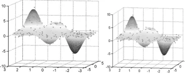
The second artificial data set was obtained by using MATLAB command “peaks (170)” to generate 28900 data points in R2. Just like our first experiment, the Gaussian noises (mean=0 and

standard deviation σ =0.4 ) were added. Similar to the first experiment, we setε =0.02,µ=1 and C = 1000. Because of storing the fully dense kernel matrix required in nonlinear ε-PSSVR, will exceed

the memory capacity and the reduced kernel technique was applied here. We randomly selected 300 points which are slightly over 10 percent of the entire training data set to form a reduced set and used the reduced kernel formulation to generate the nonlinear regression function. The resulting function of ε-PSSVR (a) and the original function

(b, without noises) were shown in Figure 5. The dots that were shown in Figure 5 form the reduced set. This result was generated in 11.362 seconds with 0.01 relative error. We also tested ε-SSVR on

his artificial data set. However, they took a much longer time to get the solution with the same level of accuracy. We summarized the numerical results of these two artificial data sets in Table4.

Figure 5: The Regression Of 3D Artificial Data Sets(A)(B)

Table4: Numerical Result For 3D Artificial Data Sets

Methods #SVs Train

Error(%)

Test

Error(%) CPU(s)

ε_-PSSVR

ε-MPSSVR 17820 17818

1.08 1.01

1.12 1.01

12.086 11.362

7. CONCLUSIONS

In this paper, we successfully obtain the polynomial smoothing function which approaches the square of ε-insensitive loss function by using

three interpolation points cubic Spline interpolation method, that is S_M2_ε-function, and proved that this function has better properties, the approximation accuracy is three order of higher than P_ε2-function

and one order of higher than S_ε2-function. As a

result, to apply 2 M

ISSN: 1992-8645 www.jatit.org E-ISSN: 1817-3195 vector regression model fitting and other related

fields.

ACKNOWLEDGEMENTS

This work was supported by the Guangdong Natural Science Foundation Project(No.S2011 010002144),The Ministry of Education, Guangdong Province, Production and Research Projects(No.2010B090400457, No.2011B090400 269 , No.2011A091000028),Guangdong Province Enterprise Laboratory Project(No.2011A091000 0 46) , the Natural Science Foundation of Dong Guan University of Technology Project (No.2010ZQ04).

REFERENCES:

[1] C. Chen and O. L. Mangasarian, “A class of smoothing functions for nonlinear and mixed complementarity problems”, Computational

Optimization and Application, Vol.5, No.5,

1996, pp.97-138.

[2] Y. B. Yuan, J. Yan and C. X. Xu, “Polynomial smooth support vector machine (PSSVM)”,

Chinese Journal of Computers , Vol. 28, No. 1,

2005, pp. 9-17.

[3] C. Chen and O. L. Mangasarian, “Smoothing methods for convex inequalities and linear complementarity problems”, Mathematical Programming, Vol. 71, 1995, pp. 51-69.

[4] C. astroNeto, M. J. Youngseon, J. Myong K. et al, “AADT prediction using support vector regression with data-dependent parameters”,

Expert Systems with Applications, Vol. 36, No.

2: PART 2 , 2009, pp. 2979-2986.

[5] C. Andreas and V. M. Arnout, “Bouligand derivatives and robustness of support vector machines for regression”, Journal of Machine

Learning Research, Vol. 9, 2008, pp. 915-936.

[6] L. Mangasarian and D. R. Musicant, “Successive overrelaxation for support vector machines”, IEEE Transactions on Neural

Networks, Vol. 10, No. 8, 1999, pp. 1032-1037.

Y. J. Lee and O. L. Mangasarian, “SSVM: A smooth support vector machine for classification”, Computational Optimization

and Applications, Vol. 22, No. 1, 2001, pp.

5-21.

[7] Y. J. Lee, W. F. Hsieh and C. M. Huang, “ε -SSVR: A smooth support vector machine for ε -insensitive regression”, IEEE Transactions on

Knowledge and Data Engineering , Vol. 17,

No. 5, 2005, pp. 5-22.

[8] C. C. Chang and C. J. Lin, LIBSVM:A library for support vector machines, software available at http://www.csie.ntu.edu.tw/~cjlin/libsvm, 2012.

[9] J Platt. Sequential minimal optimization: A fast algorithm for training support vector machines,

Advances in Kernel Methods-Support Vector Learning. MIT Press, Cambridge, MA, 1999,

PP.185-208.

[10] N. Y. Deng and Y. J. Tian. The new method in data mining-support vector machine, Press of science, 2004, pp. 244.

[11] H. Q. Yuan,W. G. Tu,J,Z. Xiong, et al, new polynomial smooth support vector machine,

Computer Science, Vol. 38, No. 3, 2011, pp.

243-247.

[12] Ren Bin, Cheng Lianglun, “Polynomial smoothing support vector regression”, Journal

of Control Theory and Applications. Vol. 28,