Stability Analysis of a Deterministic Epidemic Model in Metapopulation Setting

(1)

http://www.scirp.org/journal/apm

ISSN Online: 2160-0384 ISSN Print: 2160-0368

DOI: 10.4236/apm.2018.83011 Mar. 14, 2018 219 Advances in Pure Mathematics

Stability Analysis of a Deterministic Epidemic

Model in Metapopulation Setting

Petros Kelkile Desalegn, Samuel Mwalili, John Mango

Department of Mathematics, Pan Africa University Institute of Basic Sciences, Technology and Innovation, Nairobi, Kenya

Abstract

We present in this article an epidemic model with saturated in metapopula-tion setting. We develop the mathematical modelling of HIV transmission among adults in Metapopulation setting. We discussed the positivity of the system. We calculated the reproduction number, If R0j ≤1 for j=1, 2,3, 4,

then each infectious individual in Sub-Population j infects on average less than one other person and the disease is likely to die out. Otherwise, if

0j 1

R > for j=1, 2,3, 4, then each infectious individual in Sub-Population j infects on average more than one other person; the infection could therefore establish itself in the population and become endemic. An epidemic model, where the presence or absence of an epidemic wave is characterized by the value of R0j both ideas of the inner equilibrium point of stability properties

are discussed.

Keywords

Basic Reproduction Ratio, Lyapunov Function, Meta-Population, Disease-Free and the Endemic Equilibrium

1. Introduction

Numerous mathematical models have been developed in order to understand disease transmissions and behavior of epidemics. One of the earliest of these models as discussed by Kermack [1], by considering the total population into three classes, namely, susceptible (S) individuals, infected (I) individuals, and recovered (R) individuals which is known to us as SIR epidemic model. This SIR or SI epidemic model is very significant in todays analysis of diseases. SIR Model: The SIR model labels these three compartments S = number susceptible, I = number infectious, and R = number recovered. This is a good and simple model for many infectious diseases. Birth→_S→_I→_R→_{Death and The SI model labels}

How to cite this paper: Desalegn, P.K., Mwalili, S. and Mango, J. (2018) Stability Analysis of a Deterministic Epidemic Mod-el in Metapopulation Setting. Advances in Pure Mathematics, 8, 219-231.

https://doi.org/10.4236/apm.2018.83011

Received: November 4, 2017 Accepted: March 11, 2018 Published: March 14, 2018

http://creativecommons.org/licenses/by/4.0/

(2)

DOI: 10.4236/apm.2018.83011 220 Advances in Pure Mathematics these two compartments S = number susceptible and I = number infectious. This is a good and simple model for many infectious diseases. Birth→_S→_I→_Death.

In the mathematical epidemiology area an key concept is associated to the basic reproduction number (R0). This is defined as the second expected number produced from just a one individual in a susceptible population. For any infectious disease, one of the most key concerns is its capacity to invade a population, as studied by various authors [2]. This can be expressed by a threshold parameter: if the disease free equilibrium is locally asymptotically stable, then the disease cannot invade the population and R0<1, whereas if the number of infected individuals grows, the disease can invade the population and

0 1

R > , as studied by various authors [3].

2. Compartmental Model and Differential Equations

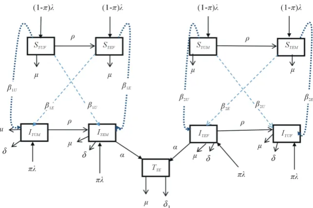
In this section, we approached this study by using SI deterministic model.

In our model system the recruitment into the susceptible human population is only by births (

λ

). The size of the human population is decreased by natural deaths (

µ

_{), infected and awareness/education. Uneducated and educated}

infected female youth move to the classes SYUF, SYEF respectively at the rate 1

β _{whereas uneducated and educated infected males youth move to the classes}

YUM

I , IYEM respectively at the rate β2 resulting in an increase in the youth infectious classes. The infectious classes are all decreased by natural deaths (

µ

₎

and disease induced deaths (

δ

, δ1). SYEF and IYEM is decreased further as a result of the infected educated, II vertical transmission and tested youths going through the Antiretroviral therapy thus moving to the treatment class TY at the rate

α

_{. We assume that once a person becomes infected with HIV they do not}

[image:2.595.214.536.492.706.2]

fully recover as there is no immunity to HIV and that only the educated and tested persons qualify the antiretroviral therapy.

(3)

[image:3.595.213.537.67.294.2] [image:3.595.219.530.330.630.2]

DOI: 10.4236/apm.2018.83011 221 Advances in Pure Mathematics

Figure 2. Schematics of the metapopulation model.

Differential Equation of the model

(

)

(

)

(

)

(

)

, , ,

1, , 1, , ,

, ,

, , ,

, 1, , 1, , ,

, ,

2, , 2,

, d

1 d

d

1 d

d

1 d

YUF i U YUM i E YEM i

i i YUF i i YUF i YUF i

YUM i YEM i

YEF i U YUM i E YEM i

YUF i i YEF i i YEF i YEF i

YUM i YEM i

YUM i U YUF i E YEF

i YUM i i

YUF i

S I I

S S S

t N N

S I I

S S S S

t N N

S I I

S

t N

λ µ β β ρ µ

λ ρ β β µ

λ β β

= − Π − − − +

= − Π + − − −

= − Π − −

(

)

(

)

(

)

,

, ,

,

, , ,

, 2, , 2, , ,

, ,

1, , 1, , ,

, ,

, , 1, d

1 d

d

d d

i

YUM i YUM i

YEF i

YEM i U YUF i E YEF i

YUM i i YEM i i YEM i YEM i

YUF i YEF i

YUM i YUM i

U U

YUM i YUF i i YEF i YUM i

YUM i YUM i

YEM E YEM

i YUM i i

S S

N

S I I

S S S S

t N N

I I

I S S I

N N

I I

I t

ρ µ

λ ρ β β µ

λ β β ρ µ δ

λ ρ β

− +

= − Π + − − −

= Π + + − + +

= Π + +

(

)

(

)

(

)

,

, 1, , ,

, ,

, 2, , 2, , ,

, ,

2, , 2, , ,

, ,

d d

d

i E YEM i

YUF i i YEF i YEM i

YEM i YEM i

YEF i YEF i

F E E

YEF

i YU i i YUM i i YEM i YEF i

YEF i YEF i

YUF i YUF i

U U

YUF

i YUM i i YEM i YUF i

YUF i YUF i

I

S S I

N N

I I

I

I S S I

t N N

I I

I

S S I

t N N

T

β α µ δ

λ ρ β β α µ δ

λ β β ρ µ δ

+ − + +

= Π + + + − + +

= Π + + − + +

(

)

,

1, , d

Y i

YEM YEF i Y i

I I T

t α α µ δ

                          

 ₌ ₊ ₋ ₊



From the proposed schematics of the compartment model shown (see Figure 1), we extracted a metapopulation model for HIV dynamics among the youth coupled with awareness/education i.e., we extended the single patch disease model to include multiple patches. A schematic of the Metapopulation Model (see

(4)

3. Positivity and Boundedness

The theory of ordinary differential equations requires that, for every set of initial conditions

(

SYUF i,0,SYEF i,0,SYUM i,0,SYEM i,0,IYUM i,0,IYEM i,0,IYEF i,0,IYUF i,0,Ti0

)

the state variables

( )

( ) ( )

(

SYUF i, t S, YEF i, t S, YUM i, t S, YEM i, t I, YUM i, t I, YEM i, t I, YEF i, t I, YUF i, t T t, i

)

of the solution must remain non-negative. Proposition 3.1. Let

( )

( ) ( )

(

SYUF i, t S, YEF i, t S, YUM i, t S, YEM i, t I, YUM i, t I, YEM i, t I, YEF i, t I, YUF i, t T t, i

)

be the solution of the system (2.0). 1) Given the initial condition

(

)

∈Ω

then there exist a unique positive solution

( )

( ) ( )

(

)

(

SYUF i, t ,SYEF i, t ,SYUM i, t ,SYEM i, t ,IYUM i, t ,IYEM i, t ,IYEF i, t ,IYUF i, t T t, i

)

for every t≥0 such that the solution will remain in Ω with probability of one.

2) The solution

(

)

(

SYUF i,,SYEF i,,SYUM i,,SYEM i,,IYUM i,,IYEM i,,IYEF i,,IYUF i,,Ti

)

is defined in the interval

[ )

0,

∞

and limt supN t

( )

4 λ µ

→∞ ≤ where

( )

( ) ( )

YUF YEF YUM YEM YUM

YEM YEF YUF

N t S t S t S t S t I t

I t I t I t T t

= + + + +

+ + + +

Proof: In (1) we let

(

)

∈Ω

Evidently, the coefficients of system (2.0) are locally Lipschitz continuous. Hence, for any given initial condition

(

)

∈Ω

there exist a unique local solution

( )

( ) ( )

(

)

(

SYUF i, t ,SYEF i, t ,SYUM i, t ,SYEM i, t ,IYUM i, t ,IYEM i, t ,IYEF i, t ,IYUF i, t T t, i

)

for every

t

∈

[ )

0,

T

, where T is the final time. Here, it can be deduced that

( )

, , , , ,

, , ,

4

YUF i YEF i YUM i YEM i YUM i

YEM i YEF i YUF i i

S t S t S t S t I t

I t I t I t T t λ

µ

+ + + +

+ + + + ≤

(5)

( ) (

)

d

N t

≤

4 λ µ

−

N

d

t

. Suppose x(t) is the solution of the differential equation

( )

(

( )

)

dN t = 4

λ

−dx t dt,

x

( )

0 =

N

( )

0

where

( )

, , , , ,

, , ,

0 0 0 0 0 0

0 0 0 0

i YUF i YEF i YUM i YEM i YUM i

YEM i YEF i YUF i i

N S S S S I

I I I T

= + + + +

+ + + +

Hence, by comparison theorem; N t

( ) ( )

x t 4λ µ

≤ ≤ _for

t

∈

[ )

0,

T

as required. Again, we can verify in (2) that

, , , , ,

, , , 1,

d 4 d

i

i i YUF i YEF i i YUM i i YME i i YUM i

i YEM i i YEF i i YUF i i i i i N

S S S S I

t

I I I T T

λ µ µ µ µ µ

µ µ µ µ δ

≤ − − − − −

− − − − −

(

1

)

₍

₎

1, 1

d d

4 4

d d

n i

i n

i

i i i i i i i i

i N N

N T N

t t λ µ δ λ µ

=

∑

=

∑

− − ≤ −

Integrating inequality (3.0) gives N t

( )

4λ

(

1 e µt

)

µ

−

≤ − for every t∈

[

0,T

]

which implies N t

( )

8λ µ

≤ _{. It can therefore be verified that the solution}

(

)

(

SYUF i,,SYEF i,,SYUM i,,SYEM i,,IYUM i,,IYEM i,,IYEF i,,IYUF i,,Ti

)

is bounded within the

interval t∈

[

0,T

]

. This implies N t

( )

4λ

(

1 e µt

)

µ

−

≤ − _{for every}

t

∈ ∞

[ )

0,

. Hence limt supN t

( )

4

λ µ

→∞ ≤ . Hence, employing the same intuition used in

proving proposition 3.1, we see that system (2.0) with non-negative initial conditions SYUF i,0≥0 , SYEF i,0≥0 , SYUM i,0 ≥0 , SYEM i,0 ≥0 , IYUM i,0≥0 ,

0

, 0

YEM i

I ≥ ,

0

, 0

YEF i

I ≥ ,

0

, 0

YUF i

I ≥ ,

0 0

i

T ≥ has a non-negative solution defined in R and the set

(

, , , , , , , ,

)

,

, , , , , ,

, ,

, , , , , , , , / 0,

0, 0, 0, 0, 0, 0,

0, 0, 0 and

YUF i YEF i YUM i YEM i YUM i YEM i YEF i YUF i i c i

YUF i YEF i YUM i YEM i YUM i YEM i

YEF i YUF i i YUF YEF YUM YEM

YUM YEM YEF Y

S S S S I I I I T S

S S S S I I

I I T S S S S

I I I I



Ω = >



> > > > > >

> > > + + +

+ + + + UF T 4

λ µ



+ = 



is invariant by system (2.0).

4. Calculation of the Basic Reproduction Number

The basic reproduction number (R0) is defined as an infections originating from an infected individual that invades a population originally of susceptible individuals. R0 is used to predict whether the epidemic will spread or die out. In the next part, we will analyze the dynamics of IYUM i, , IYEM i, , IYEF i, and

,

YUF i

(6)

DOI: 10.4236/apm.2018.83011 224 Advances in Pure Mathematics model from 2.0).

(

)

(

)

(

)

(

)

(

)

(

)

, ,

1, , ,

,

1, , , ,

,

, ,

, 1, , ,

,

1, , , ,

, , d d d d d d

YUM i U YUM i

i YUF i YUF i

YUM i

YUM i U

i YEF i YEF i i i i YUM i

YUM i

YEM i E YEM i

i YUM i i YUF i YUF i

YEM i

YEM i E

i YEF i YEF i i i i YEM i

YEM i YEF i I I N I t N I

I I I

N

I I

I N I

t N

I

N I I

N I

t

λ β

β ρ µ δ

λ ρ β

β α µ δ

λ

= Π + −

+ − − + +

= Π + + −

+ − − + +

= Π +

(

)

(

)

(

)

(

)

(

)

(

)

,

, 2, , ,

,

2, , , ,

,

, ,

2, , ,

,

2, , , ,

, , , , d d d d YEF i F E

i YU i i YUM i YUM i

YEF i

YEF i E

i YEM i YEM i i i i YEF i

YEF i

YUF i U YUF i

i YUM i YUM i

YUF i

YUF i U

i YEM i YEM i i i i YUF i

YUF i

Y i

i YEM i i YEF i I

I N I

N I

N I I

N

I I

N I

t N

I

N I I

N T

I I

t

ρ β

β α µ δ

λ β

β ρ µ δ

α α

+ −

+ − − + +

= Π + −

+ − − + +

= + −

(

µ δ_i _1,_i

)

T_{Y i}_,

                            ₊ 

The above system can be represented in matrix form as .

I = fI+vI where f is the matrix of the infection rates and v is the matrix of the transition rates.

The spectral radius of the Metzler Matrix,

(

1

)

FV

ρ

₋ −

, is defined as the largest eigenvalue of the Metzler Matrix [4]. Thus:

(

1

) (

1

)

FV FV I

ρ ₋ − _{= −} − ₋λ ₌

(

)

(

2, ,

)

,

1

, U

i YEM i YUM i

i i i YUF i

N N

R

N

β

ρ µ δ

+ =

+ +

(

)

(

1, ,

)

,

2

, E

i YEF i YUF i

i i i YEM i

N N

R

N

β

α µ δ

+ =

+ +

(

)

(

2, ,

)

,

3

, E

i YEM i YUM i

i i i YEF i

N N

R

N

β

α µ δ

+ =

+ +

(

)

(

1, ,

)

,

4

, U

i YEF i YUF i

i i i YUM i

N N

R

N

β

ρ µ δ

+ =

+ +

If R0j≤1 for j=1,2,3,4, then each infectious individual in Sub-Population

j infects on average less than one other person and the disease is likely to die out Otherwise, If R0j>1 for j=1,2,3,4 , then each infectious individual in

(7)

5. Stability of the Disease Free Equilibrium Stability

Consider the differential equation x= f t x x

( )

; , ∈Rn then a point x is Liaponouv stable if and only if for all >0 there exists

δ

>0 such that if

x

− <

y

δ

then if f x t

( )

, − f y t

( )

, < for all t≥0 . A point x is quasi-asymptotically stable if there exists

δ

>0 such that if

x

− <

y

δ

then if

( ) ( )

x t, y t, 0

ϕ

−

ϕ

→ _as t→ ∞. A point x is asymptotically stable if it is both liaponouv stable and quasi-asymptotically stable [5].

Local Asymptotic Stability

A point

x

∗ is an equilibrium point of the system if f x

( )

∗ =0.

x

∗ is locally stable if all solutions which start near

x

∗ (meaning that the initial conditions are in a neighborhood of

x

∗) remain near

x

∗ for all time. The equilibrium point

x

∗ is said to be locally asymptotically stable if

x

∗ is locally stable and, furthermore, all solutions starting near

x

∗ tend towards

x

∗ as t→ ∞ [5].

Global Asymptotic Stability

The system x∗= f t x

( )

; is globally asymptotically stable if for every trajectory

x t

( )

, we have x t

( )

→x∗ as t→ ∞ (implies

x

∗ is the unique equilibrium point) [5].

Liapunov stability

An important technique in stability theory for differential equations is one known as the direct method of Liapunov. A Liapunov function is constructed to prove stability or asymptotic stability of an equilibrium in a given region.

Definition 5.1. A positive-definite function V in an open neighborhood of the origin is said to be a Liapunov function for the autonomous differential system,

x



=

f x y

( )

,

y



=

g x y

( )

,

, if V x y

(

,

)

≤0 for all

( )

x y

,

∈

U

( )

0, 0

. If

(

,

)

0

V x y < for all

( )

x y

,

∈

U

( )

0, 0

, the function V is called a strict Liapunov

function.

Theorem 5.1. (Liapunovs Stability Theorem [6].) Let

(

0, 0

)

be an equilibrium of the autonomous system

x



=

,

f x y

( )

and let V be a positive definite 1

C

function in a neighborhood U of the origin.

1) If V x y

(

,

)

≤0 for all

(

x y,

)

∈U

(

0, 0

)

, then

(

0, 0

)

is stable.

2) If V x y

(

,

)

<0 for all

(

x y,

)

∈U

(

0, 0

)

, then

(

0, 0

)

is asymptotically stable.

3) If V x y

(

,

)

<0 for some

(

x y,

)

∈U

(

0, 0

)

, then

(

0, 0

)

is unstable. We note that in case 1 the function V is a Liapunov function and in case (2) V is a strict Liapunov function.

Here, we investigate the local stability of the disease free equilibrium point

0

E , by employing the method described in [7][8] to linearize the model system (2.0) by computing its Jacobian matrix. The Jacobian matrix is computed at disease free equilibrium point by differentiating each equation in the system with respect to the state variables SYUF,SYEF,SYUM,SYEM,IYUM,IYEM,IYEF,IYUF and

(

)

T ART

.

(8)

(

)

, , 1, 1, , , M M

YU i YE i

U E

i M i M

YU i YE i

I I

A

N N

β

ρ µ

= − − − + _,

, ,

1, 1,

, ,

M M

YU i YE i

U E

i M i M

YU i YE i

I I

B

N N

β

µ

= − − − _,

(

)

, , 2, 2, , , F F

YU i YE i

U E

i F i F

YU i YE i

I I

C

N N

β

ρ µ

= − − − + _,

, ,

2, 2,

, ,

F F

YU i YE i

U E

i F i F

YU i YE i

I I

D

N N

β

µ

= − − − _,

(

)

, , 1, 1, , , F F

YU i YE i

U U

i M i M

YU i YU i

S S

E

N N

β

ρ µ δ

= + − + + ,

(

)

, , 1, 1, , , F F

YU i YE i

E E

i M i M

YE i YE i

S S

F

N N

β

α µ δ

= + − + + _,

(

)

, , 2, 2, , , M M

YU i YE i

E E

i F i F

YE i YE i

S S

G

N N

β

α µ δ

= + − + + _,

(

)

, , 2, 2, , , M M

YU i YE i

U U

i F i F

YU i YU i

S S

H

N N

β

ρ µ δ

= + − + + _,

(

1,i

)

I= −

µ δ

+ , , 2, , M YU i U i F YU i S K N

β

= − _, , 2, , M YE i U i F YU i S L N

β

= − , , 1, 1, , , , , 1, 1, , , , 2, , , 2, , , , 1, 1, , , , 1, 1 ,

0 0 0 0 0 0

0 0 0 0 0

0 0 0 0 0 0

0 0 0 0 0

0 0 0 0 0 0

F F

YU i YU i

U E

i M i M

YU i YE i

F F

YE i YE i

U E

i M i M

YU i YE i

M YU i E i F YE i M YE i E i F YE i M M

YU i YU i

U U

i M i M

YU i YU i

M YE i E i M YE i S S A N N S S B N N S C K N S D L N

J I I

E

N N

I N

β β

ρ β β

β ρ β β β β β − − − − − − = , , , , , 2, 2, , , , , 2, 2, , ,

0 0 0 0 0

0 0 0 0 0 0

M YE i E i M YE i F F

YE i YE i

E E

i F i F

YE i YE i

F F

YU i YU i

U U

i F i F

YU i YU i

I F N I I G N N I I H N N I ρ

β β ρ

(9)

DOI: 10.4236/apm.2018.83011 227 Advances in Pure Mathematics Therefore the Jacobian J0 at the disease free equilibrium

(

)

0 YUF0, YEF0, YUM0, YEM0, YUM0, YEM0, YEF0, YUF0, E0

E = S S S S I I I I T

when

0 , , , , 0, 0, 0, 0, 0

YUF YUM

N N

E λ λ ρ λ λ ρ

ρ µ µ ρ µ µ

+ +   =  ₊ ₊    Let

(

)

, , 1, 1, , , F F

YU i YE i

U U

i M i M

YU i YU i

N N

S

N N

β

ρ µ δ

= + − + + _,

(

)

, , 1, 1, , , F F

YU i YE i

E E

i M i M

YE i YE i

N N

P

N N

β

α µ δ

= + − + + _,

(

)

, , 2, 2, , , M M

YU i YE i

E E

i F i F

YE i YE i

N N

R

N N

β

α µ δ

= + − + + _,

(

)

, , 2, 2, , , M M

YU i YE i

U U

i F i F

YU i YU i

N N

Q

N N

β

ρ µ δ

= + − + + _,

(

1,i

)

U= − µ δ+

(

)

(

)

, , 1, 1, , , , , 1, 1, , , , , 2, 2, , , 0 , , 2, 2, , ,

0 0 0 0 0 0

0 0 0 0 0

0 0 0 0 0 0

0 0 0 0 0

0 0 0 0 0 0 0 0

0 0 0 0 0 0

F F

YU i YU i

U E

i M i M

YU i YE i

F F

YE i YE i

U E

i M i M

YU i YE i

M M

YU i YU i

E U

i F i F

YE i YU i

M M

YE i YE i

E U

i F i F

YE i YU i

N N N N N N N N N N N N J N N N N S P

ρ µ β β

ρ − + − − − − − − + − − = − − − 0

0 0 0 0 0 0 0

0 0 0 0 0 0 0 0

0 0 0 0 0 0

R Q U ρ α α                                            

The characteristics equation corresponding to the above matrix

(

)

(

)

(

) (

(

)

(

)

(

)

(

)

(

)

1 2 3 4

, ,

1, 1, 5

, ,

1, 1, 6

, ,

2, 2, 7

, ,

F F

YU i YE i

U U

i M i M

YU i YU i

F F

YU i YE i

E E

i M i M

YE i YE i

M M

YU i YE i

E E

i F i F

YE i YE i

S S N N S S N N S S N N

ρ µ λ µ λ ρ µ λ µ λ

β β ρ µ δ λ

β β α µ δ λ

− + − − − − + − − −    ×__ + − + + _− _        ×__ + − + + _− _       ×_ + − + + − _   × , ,

(

)

(

)

2, 2, 8 1, 9

, ,

0

M M

YU i YE i

U U

i F i F i

YU i YU i

S S

N N

β β ρ µ δ λ µ δ λ

 

+ − + + − − + − =

 

(10)

DOI: 10.4236/apm.2018.83011 228 Advances in Pure Mathematics For E0 to be asymptotically stable, all eigenvalues i<0, (i = 1, 2, 3, 4, 5, 6, 7, 8, 9) of J₀ must be negative. From (5.0.), it is clear that λ1= −

(

ρ µ+

)

,

2

λ = −µ _, λ₃= −

₍

ρ µ+

₎

, λ4= −µ and

λ

9= −

(

µ δ

+ 1,i

)

is negative and therefore if

(

)

, ,

5 1, 1,

, ,

0

F F

YU i YE i

U U

i M i M

YU i YU i

S S

N N

λ

=

β

+

β

−

ρ µ δ

+ + < _,

(

)

, ,

6 1, 1,

, ,

0

F F

YU i YE i

E E

i M i M

YE i YE i

S S

N N

λ

=

β

+

β

−

α µ δ

+ + < _,

(

)

, ,

7 2, 2,

, ,

0

M M

YU i YE i

E E

i F i F

YE i YE i

S S

N N

λ

=

β

+

β

−

α µ δ

+ + <

and

(

)

, ,

8 2, 2,

, ,

0

M M

YU i YE i

U U

i F i F

YU i YU i

S S

N N

λ

=

β

+

β

−

ρ µ δ

+ + <

then both eigenvalues are negative. The condition λ <5 0, λ <6 0, λ <7 0 and

8 0

λ < _{implies that}

, ,

1, 1,

, ,

F F

YU i YE i

U U

i M i M

YU i YU i

S S

N N

β

+

β

< + +

ρ µ δ

,

, ,

1, 1,

, ,

F F

YU i YE i

E E

i M i M

YE i YE i

S S

N N

β

+

β

< + +

α µ δ

_,

, ,

2, 2,

, ,

M M

YU i YE i

E E

i F i F

YE i YE i

S S

N N

β

+

β

< + +

α µ δ

_,

, ,

2, 2,

, ,

M M

YU i YE i

U U

i F i F

YU i YU i

S S

N N

β

+

β

< + +

ρ µ δ

respectively. Hence the disease-free equilibrium is locally asymptotically stable if the basic reproduction number,

(

)

(

)

1, , ,

01 ,

1

U F F

i YU i YE i M

YU i

S S

R N β

ρ µ δ +

= <

+ + ,

(

)

(

)

1, , ,

02 ,

1

E F F

i YU i YE i M

YE i

S S

R N β

α µ δ +

= <

+ + ,

(

)

(

)

2, , ,

03 ,

1

E M M

i YU i YE i F

YE i

S S

R N β

α µ δ +

= <

+ +

and

(

)

(

)

2, , ,

04 ,

1

U M M

i YU i YE i F

YU i

S S

R N β

ρ µ δ +

= <

+ +

(11)

0j, 1, 2, 3, 4

R j= , and then the endemic equilibrium point exists and the infection persists in the mepopulation.

Theorem 5.2. (see Van den Driessche and Watmough [9]). The disease free equilibrium of system (2.0), E0, is locally asymptotically stable if R0<1

6. Global Stability of the Disease-Free Equilibrium

In this section, we prove that E0 is actually globally asymptotically stable when

0j 1

R ≤ . Therefore, the model (2.0) demonstrates global threshold dynamics. We shall achieve our goal by constructing an appropriate Lyapunov functional.

Theorem 6.1. The disease-free equilibrium

0 0

0 , , , , 0, 0, 0, 0, 0

YUF YUM

N N

E λ λ ρ λ λ ρ

ρ µ µ ρ µ µ

+ +

 

=  ₊ ₊ 

 

is globally asymptotically stable in 9

R₊ whenever R₀_j≤1.

Proof: We consider the Lyapunov function

( )

1 2 3 4 5

6 7 8 9

YUF YEF YUM YEM YUM

YEM YEF YUF E

L t w S w S w S w S w I w I w I w I w T

= + + + +

+ + + +

where w ii, =1, 2,, 9 are constants that would be chosen in the course of the proof. Hence, calculating the rate of change of Lalong the solution of (2.0) gives,

d d d d

d

d d d d d

YUF YEF YUM YEM

YUM YEM YEF YUF

S S S S

L L L L L

t S t S t S t S t

I I I I

L L L L L T

I t I t I t I t T t

∂ ∂ ∂ ∂ = ⋅ + ⋅ + ⋅ + ⋅ ∂ ∂ ∂ ∂ ∂ ∂ ∂ ∂ ∂ + ⋅ + ⋅ + ⋅ + ⋅ + ⋅ ∂ ∂ ∂ ∂ ∂

(

)

(

)

(

)

(

)

, ,

1 1, , 1, , ,

, ,

2 , 1, , 1, , ,

, ,

,

3 2, , 2,

, d 1 d 1 1

YUM i YEM i

U E

i YUF i i YUF i i i YUF i

YUM i YEM i

F U E

i YU i i YEF i i YEF i i YEF i

YUM i YEM i

YUF i YE

U E

i YUM i i

YUF i

I I

L

w S S S

t N N

I I

w S S S S

N N

I I

w S

N

λ β β ρ µ

λ ρ β β µ

λ β β

 

= _ − Π − − − + _

 

 

+ _ − Π + − − − _

 

+ − Π − −

(

)

(

)

(

)

, , , , , ,

4 , 2, , 2, , ,

, ,

5 1, , 1, , ,

, ,

1

F i

YUM i i i YUM i YEF i

YUF i YEF i

U E

YUM i i YEM i i YEM i i YEM i

YUF i YEF i

YUM i YUM i

U U

i YUF i i YEF i i i i YUM i

YUM i YUM i

S S

N

I I

w S S S S

N N

I I

w S S I

N N

ρ µ

λ ρ β β µ

λ β β ρ µ δ

  − +        

+ _ − Π + − − − _

 

 

+ _Π + + − + + _

 

(

)

(

)

, ,

6 , 1, , 1, , ,

, ,

7 , 2, , 2, , ,

, ,

,

8 2, ,

,

YEM i YEM i

E E

i YUM i i YUF i i YEF i i i i YEM i

YEM i YEM i

YEF i YEF i

E E

i YUF i i YUM i i YEM i i i i YEF i

YEF i YEF i

YUF i U

i YUM i

YUF i

I I

w I S S I

N N

I I

w I S S I

N N

I

w S

N

λ ρ β β α µ δ

λ β

 

+ _Π + + + − + + _

 

 

+ _Π + + + − + + _

 

+ Π + +

(

)

(

)

(

)

,

2, , ,

,

9 , , 1, ,

YUF i U

i YEM i i i i YUF i

YUF i

i YEM i i YEF i i i Y i

I

S I

N

w I I T

β ρ µ δ

α α µ δ

(12)

(

)

(

)

(

)

(

)

(

)

(

)

(

)

(

)

(

)

,

5 1 7 3 8 4 5 1 1, ,

,

6 1 1, , 2 1 , 1 ,

,

, ,

5 2 1, , 6 2 1, , 2 ,

, ,

8 3 2, d

d

YUM i U

i i i i i i i YUF i

YUM i

YEM i E

i YUF i i YUF i i YUF i

YEM i

YUM i YEM i

U E

i YEF i i YEF i i YEF i

YUM i YEM i

YU U

i

I L

w w w w w w w w S

t N

I

w w S w w S w S

N

I I

w w S w w S w S

N N

I w w

λ λ λ β

β ρ µ

β β µ

β

= − Π + − Π + − Π + −

+ − + − −

+ − ,

(

)

,

, 7 3 2, ,

, ,

F i E YEF i

YUM i i YUM i

YUF i YEF i

I

S w w S

N + − β N

(

)

(

)

(

)

(

)

(

)

(

)

(

)

(

)

(

)

(

)

(

)

,

4 3 , 3 , 8 4 2, ,

, ,

7 4 2, , 4 , 6 5 ,

,

5 , 9 6 , 5 6 ,

7 5 , 5 , 6 1, 7 ,

YUF i U

YUM i i YUM i i YEM i

YUF i

YEF i E

i YEM i i YEM i YUM i

YEF i

YUM i YEM i i YUF i

YEF i i i YEF i i i YUF i i Y i

I

w w S w S w w S

N I

w w S w S w w I

N

w I w w I w w I

w w I w I w I w T

ρ µ β

β µ ρ

µ δ α ρ

α µ δ µ δ µ δ

+ − − + −

− + + − + −

+ − − + − + − +

Choosing w1=w2=w3=w4=w5=w6=w7=w8=w9 gives the following

(

)

(

)

(

1

)

7 2

(

)

38

(

4 1,

)

9 , 5 6

YUF YEF YUM YEM YUM YEM

YEF YUF i Y i

w S w S w S w S w I w I

w I w I w T

µ µ µ µ µ δ µ δ

µ δ µ δ µ δ

− − − − − + − +

− + − + − +

It follows that Lis positive definite and d d L

t is negative definite. It can therefore be ascertained that the function is a Lyapunov function for system (2.0). Hence by Lyapunov asymptotic stability theorem [10], the equilibrium E0 is globally asymptotically stable.

7. Conclusion

In this study, we approached using deterministic model. We developed a mathematical model of HIV transmission among adults in Meta-population setting in Ethiopia. Our model captures the disease induced deaths in transmission as HIV is known to cause deaths in transmission. Mathematical analysis was done and it was established that in the absence of the disease a disease free equilibrium will always exist if R0j≤1 for j=1, 2, 3, 4. We also

established that the endemic equilibrium exists in the presence of the disease that is when R0j>1 for j=1, 2, 3, 4, with the infectious population greater

than zero. Reducing the infection in the vector population reduces R0j for

1, 2, 3, 4

j= , greatly. Thus the best methods of controlling HIV transmission is to target the Infected uneducated female youth, Infected educated female youth, Infected uneducated male youth, Infected educated male youth. R0j is

a threshold that completely determines the global dynamics of disease transmission.

Conflict of Interest

(13)

DOI: 10.4236/apm.2018.83011 231 Advances in Pure Mathematics publication of this paper.

References

[1] Kermack, W.O. and McKendrick, A.G. (1927) Contributions to the Mathematical Theory of Epidemics. Proceedings of the Royal Society A: Mathematical, Physical and Engineering Sciences, 115, 700-721.

[2] Heffernan, J.M., Smith, R.J. and Wahl, L.M. (2005) Perspectives on the Basic Re-productive Ratio. Journal of the Royal Society Interface, 2, 281-291.

https://doi.org/10.1098/rsif.2005.0042

[3] van den Driessche, P. and Watmough, J. (2003) Reproduction Ratio and Endemic Equilibria for Deterministic Models of Disease Transmission. Mathematical Sciences, 181, 25-49.

[4] Siekmann, O. and Heesterbeek, J.A.P. (2000) Mathematical of Infectious Diseases: Model Structure, Analysis and Interpretation. John Wiley and Sons, New York. [5] Cull, P. (1986) Local and Global Stability for Population Models. Biological

Cyber-netics, 54, 141-149. https://doi.org/10.1007/BF00356852

[6] Li, J. and Zou, X. (2009) Generalization of the Kermack-McKendrick SIR model to a Patchy Environment for a Disease with Latency. Mathematical Modelling of Natural Phenomena, 4, 92-118.https://doi.org/10.1051/mmnp/20094205

[7] Ngwenya, O. (2009) The Role of Incidence Functions on the dynamics of SEIR Model. Doctoral Dissertation, University of Manitoba, Canada.

[8] Tessa, O.M. (2006) Mathematical Model for Control of Measles by Vaccination. Proceedings of Mali Symposium on Applied Sciences, 2006, 31-36.

[9] van den Driessche, P. and Watmough, J. (2002) Reproduction Numbers and Sub-Threshold Endemic Equilibria for Compartmental Models of Disease Trans-mission. Mathematical Biosciences, 180, 29-48.

https://doi.org/10.1016/S0025-5564(02)00108-6