Effects of Globalization under Consistent Conjectures

Received Jan 29, 2016 / Accepted Aug 21, 2016

Editorial Académica Dragón Azteca (EDITADA.ORG)

Effects of Globalization under Consistent Conjectures

Mariel A. Leal-Coronado

1

, Arturo García-Martínez

1

, and Vyacheslav V. Kalashnikov

1,2,3 1

_{Tecnológico de Monterrey (ITESM), Campus Monterrey, Nuevo León, México 64849}

2

_{Central Economics and Mathematics Institute (CEMI), Moscow, Russia 117418}

3

_{Sumy State University, Sumy, Ukraine 40007}

[email protected], [email protected], [email protected]

Abstract. We study the effects of merging two separate markets each originally monopolized by a producer into a globalized duopoly market. We consider a linear inverse demand with cap price and quadratic cost functions. After globalization, we find the consistent conjectural variations equilibrium (CCVE) of the duopoly game. Unlike in the Cournot equilibrium, a complete symmetry (identical cost functions parameters of both firms) does not imply the strongest coincident profit degradation. For the situation where both agents are low-marginal cost firms, we find that the company with a technical advantage over her rival has a better ratio of the current and previous profits.Moreover, as the rival becomes ever weaker, that is, as the slope of the rival’s marginal cost function increases, the profit ratio improves.

Keywords: Duopoly Game, Conjectural Variations Equilibrium, Cap Price, Globalization.

1.

Introduction

The purpose of the present paper is to investigate a market with two competing producers of an identical commodity. We consider two stages: before globalization (separate markets) and after globalization (united market). Before globalization, each producer satisfies the separate demand of the market that it monopolizes. After globalization, both firms compete in a united market. This model is often said to have the structure of a pure (classic) duopoly where both companies satisfy the complete market demand.

One can find numerous studies on the effects of combining two or more markets in the literature. According to [1], there are two types of global markets: a) the free trade market which allows the existence of n different markets with a separate supplier; and b) a single integrated market in which all producers compete.

Since the 1980s, there has been a lot of research on the role of imperfect competition. This was pointed out in [2], which deals with global markets of type a). In fact, there are several works which models correspond to these type of markets. Some examples are found in [3]–[5], too. On the other hand, [1] analyzes a globalized market of type b), through a Nash-Cournot equilibrium model, whereas in [1], the authors examine cases where all producers’ profits are degraded in the same manner. For each producer, they use the ratio of the profit obtained after globalization to the profit before globalization to represent the degree of the profit degradation, and the largest of the ratios among the producers is a measure of coincident degradation. They found that under a complete symmetry, i.e., when the values of parameters of cost and demand functions are equal, all producers have profit degradation coincidently. For the model they use which boasts linear demand functions for the separated markets and the globalized market, as well as linear cost functions, under Nash-Cournot conjectures, the value of the measure of coincident degradation is the lowest (the worst) when the firms are identical.

63

As well, at the stage of globalization, when competition takes place, we raise a kind of equilibrium with consistent conjectural variations (CCVE). Conjectural Variations Equilibria (CVE) were introduced by Bowley in 1924 [6] and Frisch in 1933 [7] as another possible solution concept in static games. According to this concept, agents behave as follows as was stated in [8]: each agent chooses her most favorable action taking into account that every rival’s strategy is a conjectured function of her own strategy. In [8] and [9], we studied mixed oligopoly models with consistent conjectural variations (CCV), which correspond to the market price variations due to the change in the output level of a producer. Concepts such as exterior and interior equilibrium were introduced, and proofs of existence and uniqueness of equilibrium were presented in the above-mentioned papers. We apply these concepts in our present paper, too.

The paper is organized as follows. In Section 2, we describe the mathematical model and specify the assumptions to accept for each stage. This section shows the optimal output levels produced by each firm before globalization as well and finds the consistent conjectural variations equilibrium price and production volumes. In Section 3, we define two types of agents: low-marginal and high-low-marginal cost firms. As we study a market with 2 agents, we have four feasible situations corresponding to the possible combination of types of firms. We define the profit ratio and compute it for each situation in terms of the parameters in order to analyze the effect of the cost parameters on this ratio. To do so, we use the concept of technical advantage introduced by [10]. In this section, we also display an example which shows that, unlike the Nash-Cournot case [1], a complete symmetry does not necessarily render the worst-case ratio under consistent conjectures. Finally, in Section 4, we present our conclusions and outline our future work.

2.

Model Specification

Before globalization, consider two monopolistic markets. Each monopoly faces an active demand 𝐷𝑖, 𝑖ϵ{0,1} which does not

depend on market price and a passive demand G𝑖(𝑝𝑖) whose argument 𝑝𝑖 is the market clearing price. We will assume that in

every market the price value 𝑝𝑖 = 𝑃̅ is the cap price. This means that the demand functions have a discontinuity point (a

break) and for prices higher than 𝑃̅ the demand is zero. Therefore, the company 𝑖 output volume, 𝑞𝑖≥ 0 , will satisfy the

following inequality if the market is “balanced”:

𝑔𝑖(𝑝𝑖) + 𝐷𝑖 ≤ 𝑞𝑖 ≤ 𝐺𝑖(𝑝𝑖) + 𝐷𝑖 . (1)

Here, 𝑔𝑖(𝑝𝑖), is the right limit of the function 𝐺𝑖 at any point while the left limit of this function at each point is assumed to

coincide with its proper value.

After globalization, both firms compete in a globalized market. The consumers’ (passive) demand is described by a demand function 𝐺(𝑝𝑤 ), whose argument 𝑝𝑤 is the market clearing price. An active demand value 𝐷is non-negative and does not depend

on the market price. Here we take for granted that after globalization, the cap price will be the same as before globalization. Since the demand function has a point of discontinuity (a break at the cap price 𝑃̅ ), the balance between the demand and supply for a given price 𝑝𝑤 is described by the following (“balance”) inequality:

𝑔(𝑝𝑤 ) + 𝐷 ≤ 𝑄 ≤ 𝐺(𝑝𝑤 ) + 𝐷 . (2)

Here, 𝑔(𝑝𝑤 )is the right limit of the function 𝐺at any point 𝑝𝑤 and 𝑄 = 𝑞0 + 𝑞1.

2.1 Assumptions

Accept the following assumptions about the demand and cost functions in order to study the effects of globalization. Before Globalization

A1.1. The inverse demand function for each firm 𝑖, 𝑖 ∈ {0, 1}, is defined as follows:

𝑝𝑖(𝜃𝑖) = {

𝑃 𝑖𝑓 0 ≤ 𝜃𝑖≤ 𝑄̅ 2⁄ ;

𝑐 − 𝑑𝜃𝑖 𝑖𝑓 𝑄̅ 2⁄ < 𝜃𝑖≤ 𝑐 𝑑⁄ .

(3)

Here 𝑐 and 𝑑 are positive values, and 𝑃 = 𝑐 − 𝑑𝑄̅ 2⁄ . The total quantity demanded in the market 𝑖 at the price 𝑝𝑖 is 𝜃𝑖, which

includes the passive and the active quantities demanded.

A1.2. For each 𝑖 ∈ {0, 1}, the cost function 𝑓𝑖(𝑞𝑖) is quadratic, i.e., 𝑓𝑖(𝑞𝑖) = 1 2𝑎𝑖𝑞𝑖

2_{+ 𝑏𝑞}

𝑖 where 𝑎𝑖> 0 and 0 < 𝑏 < 𝑐.

A1.3. 𝑃 > max

64

After Globalization

A2.1. The market inverse demand function is defined as follows:

𝑝𝑤(𝜃) = {

𝑃 𝑖𝑓 0 ≤ 𝜃 ≤ 𝑄;

𝑐 − 𝑑𝜃 2⁄ 𝑖𝑓 𝑄 < 𝜃 ≤ 2𝑐 𝑑⁄ .

(4)

Here 𝑐, 𝑑, and 𝑃 are defined as in A1.1.The variable 𝜃 is the total quantity demanded (including the passive and the active demand).

Assumption A1.2 about the cost function is also made; the cost structure won’t change after globalization. As a consequence of A1.3, if 𝑞0+ 𝑞1 < 𝑄 then 𝑃 > 𝑎𝑖𝑞𝑖+ 𝑏, for at least one 𝑖, 𝑖 ∈ {0, 1}.

2.2 Objective functions of the companies

2.2.1 Before Globalization

Recall that before globalization exists a single company in each market commercializing the commodity. Company 𝑖, ( 𝑖 ∈ {0, 1}) chooses its output volume so as to maximize its net profit function: 𝜋𝑖(𝑞𝑖) = 𝑝𝑖(𝑞𝑖)𝑞𝑖 − 𝑓𝑖(𝑞𝑖).

Note that assumption A1.3 implies that the output value that maximizes the benefits cannot be less than 𝑄̅ 2⁄ . Because of that, we can rewrite the maximization problem of any firm with sub-index 𝑖 as follows:

maximize

𝑞_𝑖 𝜋𝑖(𝑞𝑖) = 𝑝𝑖(𝑞𝑖)𝑞𝑖− 𝑓𝑖(𝑞𝑖),

subject to 𝑞𝑖≥ 𝑄/2, (5)

which can be easily solved by Karush-Kuhn-Tucker (KKT) equations. The optimal output value 𝑞̅𝑖 for private firm 𝑖, 𝑖 ∈ {0, 1}

is found as:

𝑞̅𝑖=

{ 𝑐 − 𝑏

2𝑑 + 𝑎𝑖

𝑖𝑓 𝑐 − 𝑏

2𝑑 + 𝑎𝑖

>𝑄 2; 𝑄

2 𝑖𝑓

𝑐 − 𝑏 2𝑑 + 𝑎𝑖

≤𝑄

2.

(6)

2.2.2 After Globalization

After globalization, there is an integrated market where both companies compete in a classic duopoly. The price at this stage is determined in the global market, so it obeys the inverse demand function (4) cited in assumption A2.1.

The problem of each private company 𝑖 is to maximize its net profit

𝜉𝑖(𝑞𝑖) = 𝑝𝑤 (𝑄)𝑞𝑖 − 𝑓𝑖(𝑞𝑖), 𝑖 = 0,1 . (7)

The output level of each company under the assumptions made is found using the theory of [11]. As in [11], we also claim that the output volume chosen by a producer influences the market price. This can be described by a conjectured function of the variations of the price upon variations of the production volume. Then, the first order maximum condition to define the equilibrium would have the form 𝑖, 𝑖 ∈ {0, 1}:

∂𝜉𝑖

∂𝑞𝑖

= 𝑝𝑤(𝑄) +

∂𝑝𝑤(𝑄)

∂𝑞𝑖

⋅ 𝑞𝑖− 𝑎𝑖𝑞𝑖− 𝑏 {

= 0 𝑖𝑓 𝑞𝑖> 0;

≤ 0 𝑖𝑓 𝑞𝑖= 0.

(8)

As in [11], denote 𝑣𝑖= − 𝜕𝑝𝑤(𝑄) 𝜕𝑞⁄ 𝑖 . In order to describe each agent’s behavior, we need to evaluate 𝑣𝑖. The conjectured

dependence of 𝑝𝑤 on 𝑞𝑖 must account for the (local) concavity of the 𝑖 –th agent’s objective function; otherwise one cannot guarantee

that the output volumes found via the first order optimality conditions (8) maximize (but not minimize) the profit functions. For instance, it suffices to assume that the coefficient 𝑣𝑖 (from now on referred to as the 𝑖 –th agent’s influence coefficient) is

65

In [11] and [12], we defined the concept of exterior equilibrium, i.e., conjectural variations equilibrium (CVE) with the influence coefficients fixed in an exogenous mode. As the competition after globalization has been represented by the model presented in [11], the equilibrium would be found as in the mentioned publication. Theorem 1 in [11] establishes the existence and unicity of the exterior equilibrium (𝑝𝑤 ; 𝑞̃0, 𝑞̃1) under assumptions A1.2 and A2.1, and also provides the left and right

derivatives of the equilibrium price 𝑝𝑤= 𝑝𝑤(𝐷, 𝑣0, 𝑣1) with respect to 𝐷. This theorem serves as a base for the concept of

interior equilibrium, which was defined in [11] as the exterior equilibrium with consistent conjectures (influence coefficients). Under the above assumptions, according to Theorem 2 in [11], there exists interior equilibrium after globalization.

Consistent Conjectural Variations Equilibrium:

Let

𝜏 = { −∞ 𝑖𝑓 𝑝𝑤= 𝑃̅, − 2 𝑑⁄ 𝑜𝑡ℎ𝑒𝑟𝑤𝑖𝑠𝑒.

Given the previous results obtained in [11] the influence coefficient of the agent 𝑖, 𝑖 ∈ {0, 1}, after globalization is:

𝑣𝑖=

1 1 𝑣−𝑖+𝑎−𝑖− 𝜏

, 𝑖 = 0,1,

(9)

where the symbol −𝑖 represents the competitor’s sub-index.

In (9), 𝜏 ∈ [−∞, 0]. When 𝜏 = −∞, system (9) has the unique solution

𝑣

𝑖 = 0, 𝑖 ∈ {0, 1}. The latter result corresponds to the

perfect competition equilibrium (cf., [11]).

The following result was already derived and published as Theorem 3 in [11] and Theorem 4.3 in [12], including for the case of a mixed oligopoly (competition among a public firm and several private companies).

Theorem 2.1([11]-[12]). Under assumptions A1.2 and A2.1, for any 𝜏 ≥ 0, Eq. (9) has a unique solution 𝑣𝑖 = 𝑣𝑖(𝜏 ), 𝑖 ∈

{0, 1} , continuously depending upon 𝜏. Furthermore, 𝑣𝑖(𝜏 ) → 0 when 𝜏 → −∞, and strictly increases and tends up to

𝑣𝑖(𝜏 )as 𝜏 → 0, 𝑖 = 0, 1.

Therefore, the solution of the system formed by equations (9) for the firm i’s influence coefficient is:

𝑣𝑖= {

−𝑎𝑖

2 + √

𝑎𝑖2

4 +

𝛤 𝛫−𝑖

, 𝜏 = −2

𝑑;

0, 𝜏 = −∞,

(10)

i = 0,1, where 𝛤 = 𝑎𝑖+𝑎−𝑖+ 2𝑎𝑖𝑎−𝑖⁄𝑑 and 𝛫−𝑖= 2 (2 + 2

𝑑𝑎−𝑖) 𝑑⁄ .

For the interior equilibrium price 𝑝𝑤> 𝑏, Theorems 1 and 2 in [11] imply that relationship (8) defines uniquely the equilibrium

production volume𝑠 𝑞̃𝑖, 𝑖 ∈ {0, 1}, taking into account that 𝑝𝑤= 𝑃̅ implies 𝑣𝑖 = 0:

𝑞̃𝑖=

{ 𝑝𝑤− 𝑏𝑖

𝑣𝑖+ 𝑎𝑖

, 𝑝𝑤< 𝑃̅;

𝑝𝑤− 𝑏𝑖

𝑎𝑖

, 𝑝𝑤= 𝑃,̅

(11)

i = 0,1. However, assumption A1.3 entails that the total output level given by (11) at 𝑝𝑤= 𝑃̅, is greater than 𝑄̅, but at this price

the quantity demanded is at most 𝑄̅, which means that the market is not balanced. Hence, the equilibrium can be reached only when 𝑝𝑤< 𝑃̅.

In the equilibrium when 𝑝𝑤< 𝑃̅, the total supply output equals the demand in the market. Then, from A2.1, 𝑝𝑤 = 𝑐 − 𝑑𝑄 2⁄ ,

where 𝑄 = 𝑞̃0 + 𝑞̃1 . Plug in this in the equilibrium outputs (11) to obtain the total output and the equilibrium price 𝑝𝑤 . These

66

3.

Effects of Globalization on Profits

To find the effects of globalization on profits we look for the ratio of benefits. We determine conditions involving the parameters under which these ratios are greater or smaller than 1. If the profit ratio is greater than 1 for company 𝑖, 𝑖 ∈ {0, 1} we say that globalization is beneficial for this firm, and it is not otherwise, that it, if the profit ratio is less than 1. In order to do that, we first introduce the properties of companies being low-marginal, or vice versa, high-marginal cost firms.

Definition 3.1. We say that agent 𝑖 is a low-marginal cost firm (LMCF) if the marginal cost 𝑓′

𝑖(𝑞𝑖) evaluated at 𝑄̅ 2⁄ is

less than the cap price minus a proportion 𝑑 of the quantity 𝑄̅ 2⁄ , that is, 𝑓′

𝑖(𝑄̅ 2⁄ ) <

𝑃

̅

− 𝑑

𝑄̅ 2⁄ . Conversely, agent 𝑖 is a

high-marginal cost firm (HMCF) if 𝑓′

𝑖(𝑄̅ 2⁄ ) ≥

𝑃

̅

− 𝑑

𝑄̅ 2⁄ .

Before globalization, the output level produced by firm i to supply to a separate market depends on the value of the corresponding parameters. On the one hand, if firm 𝑖 is an LMCF, it produces

𝑞̅

_𝑖

=

𝑐−𝑏

2𝑑+𝑎𝑖

.On the other hand, if it is an HMCF

it supplies 𝑞̅𝑖= 𝑄̅

2. Because of that, before globalization four situations in total are feasible depending on the characteristics of

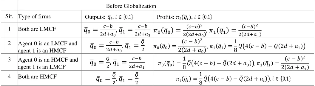
[image:5.612.48.576.324.469.2]

the firms of both markets. These situations are described in Table 1, which shows the optimal outputs and the profits for both firms.

Table 1. Possible Situations.

Before Globalization

Sit. Type of firms Outputs: 𝑞̅𝑖, 𝑖 ∈ {0,1} Profits: 𝜋𝑖(𝑞̅𝑖), 𝑖 ∈ {0,1}

1 Both are LMCF

_𝑞̅

₀

₌

𝑐−𝑏

2𝑑+𝑎0,

𝑞̅

1

=

𝑐−𝑏

2𝑑+𝑎1

𝜋

0

(𝑞̅

0

) =

(𝑐−𝑏)2

2(2𝑑+𝑎0)

, 𝜋

1

(𝑞̅

1

) =

(𝑐−𝑏)2 2(2𝑑+𝑎1)

2 Agent 0 is an LMCF and

agent 1 is an HMCF

𝑞̅

0

=

𝑐−𝑏 2𝑑+𝑎0,

𝑞̅

1

=

𝑄̅

2 𝜋0(𝑞̅0) =

(𝑐 − 𝑏)2

2(2𝑑 + 𝑎0)

, 𝜋1(𝑞̅1) =

1

8𝑄̅(4(𝑐 − 𝑏) − 𝑄̅(2𝑑 + 𝑎1)) 3 Agent 0 is an HMCF and

agent 1 is an LMCF

𝑞̅

0

=

𝑄̅ 2

, 𝑞̅

1

=

𝑐−𝑏

2𝑑+𝑎1 𝜋0(𝑞̅0) =

1

8𝑄̅(4(𝑐 − 𝑏) − 𝑄̅(2𝑑 + 𝑎0)), 𝜋1(𝑞̅1) =

(𝑐 − 𝑏)2

2(2𝑑 + 𝑎1)

4 Both are HMCF

_𝑞̅

0

=

𝑄̅ 2,

𝑞̅

1

=

𝑄̅

2 𝜋𝑖(𝑞̅𝑖) =

1

8𝑄̅(4(𝑐 − 𝑏) − 𝑄̅(2𝑑 + 𝑎𝑖)), 𝑖 ∈ {0,1}

Let 𝑅𝑖 denote the profit ratio of company 𝑖, 𝑖 ∈ {0,1} and be given by:

𝑅

𝑖

=

𝜉𝑖(𝑞̃𝑖) 𝜋𝑖(𝑞̅𝑖)

. (12)

Formula (12) would take different values according to the faced situation. 3.1 Measure of coincident profit degradation

Globalization may improve or degrade the profits of the companies. However, [1] study the cases when coincident profit degradation occurs, that is, both firms have smaller profits after globalization than before. In the above-mentioned work, the profit ratio of a producer after globalization to that before globalization is proposed as the degree of profit degradation for the producer due to globalization. They utilize the largest of the ratios of profit degradation among producers as a measure of coincident degradation. According to [1], the reason is: a smaller value of the measure is supposed to indicate stronger coincident degradation. The situation where only one of the producers suffers profit degradation cannot be considered overall coincident producer profit degradation as far as the other producer enjoys profit improvement. The measure of coincident profit degradation used in [1] for a duopoly is defined by the following equality:

𝑘𝑅 = 𝑚𝑎𝑥{𝑅0, 𝑅1}. (13)

67

is reached by a market system if, and only if the system is in complete symmetry. In the next subsection, we show how this result is not necessarily true in the case of the equilibrium with consistent conjectural variations, at least for a system of two firms with quadratic cost functions. We also describe the effect of the cost parameters values, 𝑎𝑖 and 𝑎−𝑖 on the profit ratios. In order to do

so, we use the concept of technical advantage. According to the definition of technical advantage introduced in [10], a firm has technical advantage over its rival, if it can produce the same output that its rival produces at lower marginal and total costs than its rival. We say that firm 𝑖 has technical advantage over firm (−𝑖)if 𝑎𝑖< 𝑎−𝑖.

The proofs of the propositions are exported to Appendix due to the space issues. 3.2 Situation 1

Situation 1 stated in Table 1 refers to the case when both agents are low-marginal cost firms. Substitute the profits at the equilibrium (shown in Appendix A) and the optimal profits (Table 1) into formula (12), and after some algebraic manipulations obtain:

𝑅𝑖=

2𝑑 + 𝑎𝑖

2𝑣𝑖+ 𝑎𝑖

(2 𝑑𝑣𝑖)

2

, (14)

where

𝑣

_𝑖

=

−𝑎𝑖

2

+ √

𝑎𝑖2

4

+

Γ

Κ−𝑖 according to equation (10).

Proposition 3.1. There is degradation of the profits of private firm i if, and only if

𝜆1(𝑎𝑖, 𝑎−𝑖, 𝑑) + 𝜆2(𝑎𝑖, 𝑎−𝑖, 𝑑) > 1, (15)

where 𝜆1(𝑎𝑖, 𝑎−𝑖, 𝑑), 𝜆2(𝑎𝑖, 𝑎−𝑖, 𝑑) ∈ (0,1) are continuous functions specified in Appendix A.

Proof. See Appendix B. Coincident degradation of the benefits occurs when inequality (15) is satisfied for both 𝑖 = 0, 1. The degradation or increase of company i’s profit depends not only on the cost parameters of the same company but also on the cost parameters of the other agent.

Proposition 3.2. The profit ratio of competitor 𝑖 increases if 𝑎−𝑖 grows.

Proof. See Appendix B. Proposition 3.2 states that the larger the coefficient of the quadratic term of the rival’s cost function, the lower the profit degradation for producer 𝑖 (or, its profits may even increase). The proof of Proposition 3.2 shows that the increase of the parameter 𝑎−𝑖 of the cost function of the rival affects positively the profit ratio of player 𝑖, as expected. However, the

parameter 𝑎𝑖 of its own cost function has an ambiguous effect on this ratio. In order to show that, calculate the derivative of

𝑅𝑖 with respect to 𝑎𝑖

∂𝑅𝑖

∂𝑎𝑖

= 𝑣𝑖

𝑑2_{(𝑑 + 𝑎}

−𝑖)(2𝑣𝑖+ 𝑎𝑖)3

𝜒𝑖(𝑎𝑖, 𝑎−𝑖, 𝑑) , (16)

where 𝜒𝑖(𝑎𝑖, 𝑎−𝑖, 𝑑) is a continuous function specified in Appendix A . The sign of this derivative is the same as the sign of

𝜒𝑖(𝑎𝑖, 𝑎−𝑖, 𝑑). In order to describe the behaviour of 𝜒𝑖(𝑎𝑖, 𝑎−𝑖, 𝑑), let 𝑎𝑖 = 𝜌𝑎−𝑖 and 𝑑 = 𝜎𝑎−𝑖; 𝜌, 𝜎 > 0. By substituting

them in 𝜒𝑖, we have: 𝜒𝑖(𝜌, 𝜎, 𝑎−𝑖) = 𝑎−𝑖4 𝜒̃𝑖(𝜌, 𝜎), where 𝜒̃𝑖(𝜌, 𝜎) is a continuous function of two variables specified in

Appendix A.

In general, the sign of 𝜒̃𝑖 depends on both values 𝜌 and 𝜎. However, in particular, we can say that χ̃i shows various types of

behavior when 𝜌 takes values around zero, however 𝜒̃𝑖→ 0 when 𝜌 → 0. While 𝜌 is cut off from zero, that is, if 𝜌 ≥ 𝜌̅1> 0,

then 𝜒̃𝑖 takes negative values, for any value of 𝜎 > 0. That is, a little increments in 𝑎𝑖 affect negatively the profit ratio 𝑅𝑖,

regardless of whether firm 𝑖 has technical advantage over her rival or not, while the value of 𝑑 doesn’t exceed 𝜌̅1 times 𝑎−𝑖 (in

this case, 𝑑 may also be less than 𝑎−𝑖, but remember that the behavior of 𝜒 is ambiguous when 𝜌 is very close to zero). If 𝑠 ≤

1, which means that the rival firm (−𝑖) has no technical advantage over firm 𝑖, the effect of little increments in 𝑎𝑖 is positive

68

For the current situation, the profits of the weaker firm (−𝑖) are degraded after globalization. Another important fact is that if a firm has a technical advantage over the other, the degradation of her own profit due to globalization (if the latter happens at all) is lower than the profit degradation of the other firm. Even more, the profits of firm 𝑖 can increase. These results are summarized in Proposition 3.3.

Proposition 3.3. If 𝑎𝑖 < 𝑎−𝑖, i.e., competitor 𝑖 has technical advantage over (−𝑖), then

a) 𝑅−𝑖< 1;

b) 𝑅−𝑖< 𝑅𝑖.

Proof. See Appendix B. Note that if we consider the case where there is coincident degradation of the profits, the measure of the latter in this case would equal 𝐾𝑅 _{= 𝑅}

𝑖, i.e., the profit degradation of the firm with the technical advantage.

Under the complete symmetry, both producers suffer coincident profit degradation. This result is the same as in [2] and is stated in Proposition 3.4:

Proposition 3.4. If the firms are symmetric (𝑎𝑖 = 𝑎−𝑖 = 𝑎) the ratio of both firms is given by

𝑅 = 2𝑑 + 𝑎

2√𝑎₄2+𝑎𝑑_{2 (} 𝑎 𝑎

2+ √

𝑎2

4 +

𝑎𝑑 2 )

2

.

(17)

This resulting value is less than 1 for any positive values of 𝑎 and𝑑, which means that globalization degrades profits for each company when both firms face the same costs.

Proof. See Appendix B. In contrast to [1], the latter is not necessarily the worst case under consistent conjectures. We introduce a numerical example to show it. In the following examples, we compute, together with the consistent conjectural variations equilibrium (CCVE), the equilibrium under Nash-Cournot conjectures considering the quadratic cost functions. In [1], the cost function is linear. Nevertheless, our examples with quadratic costs show that a complete symmetry implies the worst-case ratio under Nash-Cournot conjectures, too.

Example 1. Consider a duopoly with c = 50, 𝑑 = 10, 𝑃 ̅ = 30, 𝑄̅ = 4, 𝑏 = 1, and 𝑎0 = 0.1. Table 2 (which has been

exported to Appendix A due to the space issues), simulates Situation 1 for the above-given values of the parameters and different values of the parameter 𝑎1, starting with 𝑎1 = 0.06 and increasing with a mesh of 0.02. The above-mentioned table

shows the influence coefficients in the case of CCVE, while the values of the influence coefficients at the Nash-Cournot equilibrium are always 𝑣0 = 𝑣1 = − 𝑑 2⁄ . The minimal value of the measure 𝑘𝑅 among the values presented in Table 2 is

achieved when 𝑎1 = 0.06, 𝑘𝐶𝑉𝑅 = 0.23021, which means that the worst case is not the one where the firms are symmetric,

unlike the Nash-Cournot case in which the worst case ratio is obtained when 𝑎1= 𝑎0 = 0.1. In the CCVE, as long as firm 1

has technical advantage over firm 0, 𝑘𝐶𝑉𝑅 = 0.23021 (when 𝑎1= 𝑎0, 𝑘𝐶𝑉𝑅 = 𝑅1= 𝑅0). With regard to 𝑅1, notice that 𝜌 =

10 = 100 > 𝜌̅2 . Therefore, at least when firm 0 has no technical advantage over firm 1 (𝜎 ≤ 1), 𝑅1 will increase along

with 𝑎1. This explains why a complete symmetry does not necessarily entail the worst case ratio in for conjectural CVEs.

However, in Example 2 where 𝑐 = 50, 𝑑 = 0.1, 𝑃 ̅ = 49.8, 𝑄̅ = 4, 𝑏 = 1, and 𝑎0 = 0.1, the profit ratio of firm

1 decreases as it loses the technical advantage and becomes weaker (𝜌 = 0.1 = 1), whereas the profit ratio of firm 0 increases as 𝑎1 grows. In this case, the worst measure occurs when the firms are symmetric. These results are found in Table 3 also

exported to Appendix. 3.2 Situations 2 and 3

69

𝑅0=

2𝑑 + 𝑎0

2𝑣0+ 𝑎0

(2 𝑑𝑣0)

2

, 𝑅1=

1

2(2𝑣1+ 𝑎1)((𝑐 − 𝑏)

2 𝑑𝑣1)2

𝑄

2(2𝑑 + 𝑎1) (

𝑐 − 𝑏 2𝑑 + 𝑎1−

1 2

𝑄 2)

. ₍₁₈₎

Here, propositions 3.1 and 3.2 are still valid for firm 0 because the formulas of the profit ratio for firm 0 from equations (18) are identical to formulas (14). Firm 0 would face degradations of her profits if, and only if (15) holds. The profit ratio of firm 0 increases with respect to 𝑎1. The larger the value of 𝑎1 the higher is the profit ratio for firm 0. The latter means that if

globalization damages the profits of firm 0, the degradation would not be too strong as it would be with a smaller value of 𝑎1.

For firm 1, the higher values of the slope of the rival’s marginal cost would result in a better profit ratio as stated in Proposition 3.5.

Proposition 3.5. Profit ratio of competitor 1increases on 𝑎0.

Proof. See Appendix C.

3.3 Situation 4

In Situation 4 from Table 1, both producers are high-marginal cost firms. Substituting the equilibrium and optimal values in formula (12), after simple algebraic manipulations one obtains for 𝑖 = 0, 1:

𝑅𝑖=

1

2(2𝑣𝑖+ 𝑎𝑖)((𝑐 − 𝑏)

2 𝑑𝑣𝑖)2

𝑄

2(2𝑑 + 𝑎𝑖)(_{2𝑑 + 𝑎}𝑐 − 𝑏 𝑖−

1 2 𝑄 2)

.

(19)

Proposition 3.6. The profit of competitor i increases together with 𝑎−𝑖.

Proof. See Appendix D. Therefore, the effect of increase of the quadratic cost coefficient 𝑎−𝑖 on the rival’s profit (player 𝑖) is positive.

4.

Conclusions and Future Work

In this paper, we examine consistent conjectural variations equilibrium (CCVE) for a duopoly in a market of a homogeneous product. We study the effects of uniting two separate markets each monopolized by a producer: after globalization, both firms compete in one common market. Our model assumes an inverse demand function with a cap price and quadratic cost functions of both agents. Similar to previous studies, we investigate if the companies lose or gain due to globalization by evaluating their profit ratios, i.e., the ratios of their net profits after and before entering the common market. For the situations where both agents are low-marginal cost firms, we find that the company with a technical advantage over her rival has a better profit ratio. In addition, as the rival becomes weaker, this is, as the slope of the rival’s marginal cost function increases, the agent’s profit ratio enhances, too. Moreover, when both agents are low-marginal cost firms, at least the weaker company suffers degradation of her profits due to the globalization.

Unlike the previous study [1] which considers Nash-Cournot equilibrium, we show with an example that the complete symmetry of the agents does not always provide the worst case (the lowest profit ratio) in the case of CCVE. As a consequence, we demonstrate that under consistent conjectures it is important to analyze not only the case where firms are symmetrical, although this leads us to deal with more complicated or even intractable problems.

In our forthcoming papers, we are going to analyze a system with a public firm whose maximized objective is distinct from its net profit.

Acknowledgments

70

References

1. Kameda, Hisao, & Ui, Takashi: Effects of symmetry on globalizing separated monopolies to a Nash-Cournot oligopoly. International Game Theory Review, 14(2), 1-15 (2012).

2. Brander, J.A., & Spencer, B.J.: Intra-industry trade with Bertrand and Cournot oligopoly: The role of endogenous horizontal product differentiation. Research in Economics, 69(2), 157-165 (2015).

3. Brander, J.A.: Intra-industry trade in identical commodities. Journal of International Economics, 11(1), 1-14 (1981).

4. Brander, J.A., & Krugman, P.: A “reciprocal dumping” model of international trade. Journal of International Economics, 15(3), 313-321 (1983).

5. Yilmazkuday, D., & Yilmazkuday, H.: Bilateral versus multilateral free trade agreements: A welfare analysis. Review of International Economics, 22(3), 513-535 (2014).

6. Bowley, A.L.: The mathematical groundwork of economics. Oxford: Clarendon Press (1924).

7. Frisch, R.: Monopoly - polypoly – the concept of force in the economy, National International Economics Papers, London Macmillan, 1, 23-36 (1951) (Translation by W. Beckerman).

8. Kalashnikov, V. V., Bulavsky, V. A., Kalashnykova, N. I., & Castillo, F.J.: Mixed oligopoly with consistent conjectures. European Journal of Operational Research, 210(3), 729-735 (2011).

9. Kalashnykova, N. I., Kalashnikov, V.V., & Montantes, M.A.: Consistent conjectures in mixed oligopoly with discontinuous demand function. In: Intelligent Decision Technologies (J. Watada, T. Watanabe, G. Phillips-Wren, R. J. Howlett, and L. C. Jain, eds.), 15, 427-436, (2012). 10. Flores, D., & García, A.: On the output and welfare effects of a non-profit firm in a mixed duopoly: A generalization. Economic Systems,

40(4): 631-637 (2016).

11. Kalashnikov, V.V., Bulavsky, V.A., Kalashnikov-Jr., V.V., & Kalashnykova, N.I.: Structure of demand and consistent conjectural variations equilibrium (CCVE) in a mixed oligopoly model. Annals of Operations Research, 217(1), 281-297 (2014).

12. Kalashnykova, N.I., Bulavsky, V.A., Kalashnikov, V.V., & Castillo-Pérez, F.J.: Consistent conjectural variations equilibrium in a mixed duopoly. Journal of Advanced Computational Intelligence and Intelligent Informatics, 15(2), 425-432 (2011).

5.

Appendices

5.1 Appendix A

Profits before globalization

𝜋𝑖=

{

(𝑐 − 𝑏)2

2(2𝑑 + 𝑎𝑖)

, 𝑖𝑓 𝑐 − 𝑏 2𝑑 + 𝑎𝑖

>𝑄̅ 2; 1

8𝑄̅(4(𝑐 − 𝑏) − 𝑄̅(2𝑑 + 𝑎𝑖)), 𝑖𝑓

𝑐 − 𝑏 2𝑑 + 𝑎𝑖

≤𝑄̅ 2.

(20)

Equilibrium price, outputs, and profits. We know from (9) that ∑ 1

𝑣𝑗+𝑎𝑗

1

𝑗=0 =

1 𝑣𝑖+𝑎𝑖+

1 𝑣𝑖−

2

𝑑, 𝑖 ∈ {0,1}. After some

algebraic manipulations one yields:

𝑄 =

∑ _𝑣𝑐 − 𝑏

𝑗+ 𝑎𝑗 1

𝑗=0

𝑑 2(

1 𝑣𝑖+ 𝑎𝑖+

1 𝑣𝑖)

, _𝑝

𝑤= 𝑐 −

∑ _𝑣𝑐 − 𝑏

𝑗+ 𝑎𝑗 1

𝑗=0

1 𝑣𝑖+ 𝑎𝑖+

1 𝑣𝑖

, (21)

𝜉𝑖(𝑞𝑖 ~

) = (2𝑣𝑖(𝑐 − 𝑏))

2

2𝑑2_(2𝑣 𝑖+ 𝑎𝑖)

. (22)

Profit Ratios in Situation 1

From (8), 𝑝𝑤= (𝑣𝑖+ 𝑎𝑖)𝑞̃ + 𝑏, and from 𝑖 A1.1, 𝑝𝑖(𝑞_𝑖) = 𝑐 − 𝑑𝑞_𝑖. Plug in these values in (12) and note that

(𝑐 − 𝑑𝑞_𝑖)𝑞_𝑖−1

2𝑎𝑖𝑞𝑖 2

− 𝑏𝑞_𝑖=1

2 (𝑐−𝑏)2 (2𝑑+𝑎_𝑖)=

1

2(2𝑑 + 𝑎𝑖)𝑞𝑖 2

, then (12) can be rewritten as

𝑅

_𝑖

=

2𝑣𝑖+𝑎𝑖

2𝑑+𝑎𝑖

(

𝑞𝑖̃ 𝑞̅𝑖

)

2

.

In the equilibrium, when 𝑝𝑤< 𝑃, the total supply output equals the demand in the market. Then, from A2.1, 𝑝𝑤= 𝑐 − 𝑑 2𝑄,

71

Insert the equilibrium outputs in (11) to obtain the total output and the equilibrium price 𝑝𝑤:

𝑄 = 𝑝

𝑤

∑

1 𝑣𝑗+𝑎𝑗 1

𝑗=0

−

∑

𝑏

𝑣𝑗+𝑎𝑗 1

𝑗=0

.

Then

𝑄 =

∑ 𝑐−𝑏 𝑣𝑗+𝑎𝑗 1 𝑗=0 1+𝑑 2∑ 1 𝑣𝑗+𝑎𝑗 1 𝑗=0

.

We know from (9) that

∑

1

𝑣𝑗+𝑎𝑗 1

𝑗=0

=

1 𝑣𝑖+𝑎𝑖

+

1 𝑣𝑖

−

2

𝑑

, 𝑖 ∈ {0,1}

, hence

𝑄 =

∑ 𝑐−𝑏 𝑣𝑗+𝑎𝑗 1 𝑗=0 𝑑 2 1 𝑣𝑖+𝑎𝑖+ 1 𝑣𝑖

. The equilibrium price 𝑝𝑤= 𝑐 − 𝑑𝑄 2⁄ can be plugged in (11), hence the output values ratio of firm 𝑖 is:

𝑞̃𝑖 𝑞̅𝑖

=

2𝑑+𝑎𝑖 𝑣𝑖+𝑎𝑖

−

(2𝑑+𝑎𝑖)(∑ 𝑐−𝑏 𝑣𝑗+𝑎𝑗 1 𝑗=0 ) (𝑐−𝑏)(2+𝑎𝑖 𝑣𝑖) .

Substitute this ratio in

𝑅

_𝑖

=

2𝑣𝑖+𝑎𝑖

2𝑑+𝑎𝑖

(

𝑞̃𝑖 𝑞̅𝑖

)

2

and after a little of algebra obtain

𝑅

_𝑖

=

2𝑑+𝑎𝑖

2𝑣𝑖+𝑎𝑖

(1 −

𝑣𝑖 𝑣−𝑖+𝑎−𝑖

)

2

.

Note from (9) that 𝑣𝑖

𝑣−𝑖+𝑎−𝑖

= 1 −

2

𝑑

𝑣

𝑖. Then

𝑅

𝑖

=

2𝑑+𝑎𝑖 2𝑣𝑖+𝑎𝑖

(

2 𝑑

𝑣

𝑖

)

2

The desired result is obtained by plugging in the influence coefficients (10) in the last formula for 𝑅𝑖.

Functions omitted in text for space issues

𝜆1(𝑎𝑖, 𝑎−𝑖, 𝑑) =

( 2√𝑎𝑖

2

4 +

Γ 𝐾−𝑖

2𝑑 + 𝑎𝑖

)

1 2

𝜆2(𝑎𝑖, 𝑎−𝑖, 𝑑) = 1 −

2

𝑑(−

𝑎𝑖

2 + √

𝑎_𝑖2

4 +

Γ 𝐾−𝑖

)

𝜒𝑖(𝑎𝑖, 𝑎−𝑖, 𝑑) = −(8𝑎2𝑑3+ 6𝑎𝑖𝑑2(3𝑎2+ 𝑑) + 𝑎𝑖2𝑑(14𝑎2+ 9𝑑) + 4𝑎𝑖3(𝑎2+ 𝑑)) + (2𝑑2(3𝑎2+ 𝑑)

+ 𝑎𝑖𝑑(10𝑎2+ 7𝑑) + 4𝑎𝑖2(𝑎2+ 𝑑))√

𝑑 + 𝑎𝑖

𝑑 + 𝑎2

(𝑑𝑎𝑖+ 𝑑𝑎2+ 𝑎1𝑎−𝑖)

𝜒̃𝑖(𝜌, 𝜎) = −(8𝜌3+ 4(𝜌 + 3)𝜌2𝜎 + 2(𝜌 + 2)𝜌𝜎2)

− (2(𝜌 + 3)𝜌2+ 4(𝜌 + 1)𝜎2+ (7𝜌 + 10)𝜌𝜎) (𝜎 − √(𝜌 + 𝜎) ( 𝜌

[image:10.612.49.515.83.267.2]

1 + 𝜌+ 𝜎))

Table 2. Example 1

Table 1. Example 1: 𝑐 = 50, 𝑑 = 10, 𝑃̅ = 30, 𝑄̅ = 4, 𝑏 = 1 and 𝑎0 = 0.1

𝑎1 𝑣0 𝑣1 𝑅0𝐶𝑉 𝑅1𝐶𝑉 𝑘𝐶𝑉𝑅 𝑅0𝐶 𝑅1𝐶 𝑘𝐶𝑅

[image:10.612.69.533.295.522.2]

[image:11.612.109.503.97.181.2]

72

Table 3. Example 2

Table 1. Example 2: 𝑐 = 50, 𝑑 = 0. 1, 𝑃̅ = 49.8, 𝑄̅ = 4, 𝑏 = 1 and 𝑎0 = 0.1

𝑎1 𝑣0 𝑣1 𝑅0𝐶𝑉 𝑅1𝐶𝑉 𝑘𝐶𝑉𝑅 𝑅0𝐶 𝑅1𝐶 𝑘𝐶𝑅

0.06 0.03292 0.03633 0.78401 1.03483 1.03483 0.83424 1.07555 1.07555 0.08 0.03498 0.03649 0.86406 0.97464 0.97464 0.90354 1.01047 1.01047 0.10 0.03660 0.03660 0.92820 0.92820 0.92820 0.96000 0.96000 0.96000 0.12 0.03790 0.03670 0.98068 0.89125 0.98068 1.00682 0.91973 1.00682 0.14 0.03898 0.03677 1.02439 0.86112 1.02439 1.04625 0.88685 1.04625

5.1 Appendix B. Proofs for Situation 1

Proof of Proposition 3.1. We say that profit degrades when the benefits earned after globalization are less than before, i.e. 𝑅𝑖<

1. As all parameters are positive formula 𝑅𝑖< 1 is equivalent to

(

2

𝑑

(−

𝑎𝑖

2

+ √

𝑎_𝑖2

4

+

Γ 𝐾−𝑖

))

2

<

2(√𝑎𝑖 2 4+

Γ 𝐾−𝑖)

2𝑑+𝑎𝑖

which leads to (15).

From (9), 𝑣𝑖

𝑣−𝑖+𝑎−𝑖

= 1 −

2

𝑑

𝑣

𝑖. Recall that 𝑣𝑖> 0, 𝑖 = 0,1, if

𝜏 = −

2

𝑑, and the demand and cost functions’ parameters are

also positive, then

0 < 𝑣

_𝑖

<

𝑑

2. Hence, given (10), we have

0 < 2√

𝑎_𝑖2

4

+

Γ

𝐾−𝑖

< 𝑑 + 𝑎

𝑖

, therefore

0 <

(

2(√𝑎𝑖 2 4+

Γ 𝐾−𝑖)

2𝑑+𝑎𝑖

)

1/2

< 1

.

Assumptions A1.2 and A2.2 ensure that both firms actually produce maintain nonzero output levels before and after globalization, then 𝑞̃𝑖

𝑞̅𝑖

> 0

. Since 𝑑, 𝑎𝑖, 𝑣𝑖 are positive, the product 2𝑣𝑖+𝑎𝑖

2𝑑+𝑎𝑖

(

𝑞̃𝑖 𝑞̅𝑖

)

is positive, too. Similar to the proofs in

Appendix A, substitute the value of 𝑞̃𝑖

𝑞̅𝑖

in the formulas for the ratios and find 2𝑣𝑖+𝑎𝑖

2𝑑+𝑎𝑖

(

𝑞̃𝑖 𝑞̅𝑖

) =

2

𝑑

𝑣

𝑖

> 0

. Therefore, the second

element of the sum in (15) is also smaller than 1.

∎

Proof of Proposition 3.2. Differentiate (14) by 𝑎−𝑖, and a simplification yields ∂𝑅𝑖 ∂𝑎−𝑖

=

2𝑑+𝑎𝑖

4(√𝑎𝑖 2 4+

Γ 𝐾−𝑖)

3

(

2 𝑑

)

2

(

Γ

𝐾−𝑖

) ⋅

𝐾𝑖 𝐾_−𝑖2

> 0

∎

Proof of Proposition 3.3.

a) We want to show that, if 𝑎𝑖< 𝑎−𝑖 then

𝑅−𝑖=

2𝑑 + 𝑎−𝑖

2𝑣−𝑖+ 𝑎−𝑖

(2 𝑑𝑣−𝑖)

2

< 1. (23)

Expression (23) is equivalent to

(2𝑑 + 𝑎−𝑖)(𝑣−𝑖)2< (2𝑣−𝑖+ 𝑎−𝑖) (

𝑑 2)

2

. (24)

73

(2𝑑 + 𝑎−𝑖)(𝑎𝑖(2𝑎−𝑖(𝑑 + 𝑎−𝑖) + 𝑑2) + 𝑎−𝑖𝑑(2𝑎−𝑖+ 𝑑))

4(𝑑 + 𝑎𝑖)

− (2𝑑𝑎−𝑖+ 𝑎−𝑖2 )√

𝑎−𝑖2

4 +

𝑑 (𝑎−𝑖+ 𝑎𝑖+_𝑑2𝑎𝑖𝑎−𝑖)

2 (2 +2_𝑑𝑎𝑖)

<1 2𝑑

2_√𝑎−𝑖2

4 +

𝑑 (𝑎−𝑖+ 𝑎𝑖+2_𝑑𝑎𝑖𝑎−𝑖)

2 (2 +_𝑑2𝑎𝑖)

,

(25)

which is tantamount to

(2𝑑 + 𝑎−𝑖)(𝑎𝑖(2𝑎−𝑖(𝑑 + 𝑎−𝑖) + 𝑑2) + 𝑎−𝑖𝑑(2𝑎−𝑖+ 𝑑))

4(𝑑 + 𝑎𝑖)

< ((2𝑑𝑎−𝑖+ 𝑎−𝑖2 ) +

1 2𝑑

2_{) √}𝑎−𝑖2

4 +

𝑑 (𝑎−𝑖+ 𝑎𝑖+

2 𝑑𝑎𝑖𝑎−𝑖)

2 (2 +2_𝑑𝑎𝑖)

.

(26)

Note that both sides of the inequality are positive, so we can square inequality (26) and after some algebraic manipulations obtain the following equivalent relationship:

(𝑎−𝑖+ 𝑑)(2𝑎−𝑖(𝑎−𝑖+ 2𝑑) + 𝑑2)2(𝑎𝑖+ 𝑑)(𝑎𝑖𝑑 + 𝑎−𝑖(𝑎𝑖+ 𝑑)) > (𝑎−𝑖+ 2𝑑)2(𝑎𝑖(2𝑎−𝑖(𝑎−𝑖+ 𝑑) + 𝑑2) +

𝑎−𝑖𝑑(2𝑎−𝑖+ 𝑑))2, (27)

or, which is the same,

(𝑎−𝑖+ 𝑎𝑖)𝑑7+ (5𝑎−𝑖2 + 3(𝑎−𝑖− 𝑎𝑖)𝑎𝑖)𝑑6+ 2𝑎−𝑖(2𝑎−𝑖2 + (𝑎−𝑖− 𝑎𝑖)(3𝑎𝑖+ 2(𝑎−𝑖+ 𝑎𝑖)))𝑑5+ 𝑎−𝑖2 (𝑎−𝑖2

+ (𝑎−𝑖− 𝑎𝑖)(10𝑎𝑖+ 2(𝑎−𝑖+ 𝑎𝑖)))𝑑4+ 4𝑎−𝑖3 (𝑎−𝑖− 𝑎𝑖)𝑎𝑖𝑑3> 0.

(28)

Inequality (28) is true since 𝑎𝑖< 𝑎−𝑖.

∎ b) Let 𝑎−𝑖= 𝑎. Then, after some manipulations:

𝑅𝑖=

(2𝑑 + 𝑎𝑖) (𝑎𝑖− √

𝑑 + 𝑎𝑖

𝑑 + 𝑎 √𝑑𝑎 + 𝑑𝑎𝑖+ 𝑎𝑎𝑖) 2

𝑑2_{√𝑑 + 𝑎}𝑖

𝑑 + 𝑎 √𝑑𝑎 + 𝑑𝑎𝑖+ 𝑎𝑎𝑖

,

𝑅−𝑖=

(2𝑑 + 𝑎) (𝑎 − √_{𝑑 + 𝑎}𝑑 + 𝑎

𝑖√𝑑𝑎 + 𝑑𝑎𝑖+ 𝑎𝑎𝑖) 2

𝑑2_√𝑑 + 𝑎

𝑑 + 𝑎𝑖√𝑑𝑎 + 𝑑𝑎𝑖+ 𝑎𝑎𝑖

.

In this situation, 𝑅−𝑖< 𝑅𝑖 if

𝑑 + 𝑎

2𝑑 + 𝑎(√

𝑑 + 𝑎𝑖

𝑑 + 𝑎√𝑎𝑑 + 𝑎𝑖𝑑 + 𝑎𝑎𝑖− 𝑎𝑖)

2

> 𝑑 + 𝑎𝑖 2𝑑 + 𝑎𝑖

(√𝑑 + 𝑎

𝑑 + 𝑎𝑖

√𝑎𝑑 + 𝑎𝑖𝑑 + 𝑎𝑎𝑖− 𝑎) 2

. (29)

The last inequality is obtained by simplifying the terms in the original 𝑅−𝑖< 𝑅𝑖. Note that if 𝑎𝑖< 𝑎, then

𝑑 + 𝑎𝑖

2𝑑 + 𝑎𝑖

< 𝑑 + 𝑎

74

Also, if 𝑎𝑖< 𝑎, then

𝑎𝑖 𝑎𝑖+𝑑

<

𝑎

𝑎+𝑑, because

𝑔(𝑥) =

𝑥

𝑥+𝑑 is an increasing function by 𝑥, with 𝑑 > 0. Multiply both sides by

𝑎 − 𝑎𝑖> 0 to get 𝑎𝑖

𝑎𝑖+𝑑

(𝑎 − 𝑎

𝑖

) <

𝑎

𝑎+𝑑

(𝑎 − 𝑎

𝑖

)

, which is equivalent to

𝑎

𝑖

(

𝑎+𝑑

𝑎𝑖+𝑑

− 1) < 𝑎 (1 −

𝑎𝑖+𝑑

𝑎+𝑑

)

. This

inequality is tantamount, after some algebra, to:

(𝑎 − 𝑎𝑖)2> ((√

𝑑 + 𝑎 𝑑 + 𝑎𝑖

− √𝑑 + 𝑎𝑖

𝑑 + 𝑎) √𝑑𝑎 + 𝑑𝑎𝑖+ 𝑎𝑎𝑖)

2

.

Because 𝑎 − 𝑎𝑖> 0, which implies that

√

𝑑+𝑎 𝑑+𝑎𝑖

− √

𝑑+𝑎𝑖

𝑑+𝑎

> 0

, we have 𝑎 − 𝑎𝑖> (√ 𝑑+𝑎 𝑑+𝑎_𝑖− √

𝑑+𝑎_𝑖

𝑑+𝑎) √𝑑𝑎 + 𝑑𝑎𝑖+ 𝑎𝑎𝑖

. Hence,

(√

𝑑+𝑎𝑖

𝑑+𝑎

) √𝑑𝑎 + 𝑑𝑎

𝑖

+ 𝑎𝑎

𝑖

− 𝑎

𝑖

> (√

𝑑+𝑎

𝑑+𝑎𝑖

) √𝑑𝑎 + 𝑑𝑎

𝑖

+ 𝑎𝑎

𝑖

− 𝑎

. Note that both sides are positive, therefore:

(√𝑑 + 𝑎𝑖

𝑑 + 𝑎 √𝑎𝑑 + 𝑎𝑖𝑑 + 𝑎𝑎𝑖− 𝑎𝑖)

2

> (√𝑑 + 𝑎 𝑑 + 𝑎𝑖

√𝑎𝑑 + 𝑎𝑖𝑑 + 𝑎𝑎𝑖− 𝑎) 2

. (31)

Inequalities (30) and (31) combined together imply the desired relationship (29).

∎

Proof of Proposition 3.4.

As 4𝑎6_{+ 16𝑎}5_{𝑑 + 20𝑎}4_𝑑2_{+ 8𝑎}3_𝑑3_{< 4𝑎}6_{+ 16𝑎}5_{𝑑 + 20𝑎}4_𝑑2_{+ 8𝑎}3_𝑑3_{+ 𝑎}2_𝑑4 _{then ((2𝑎}2_{+ 2𝑎𝑑)√𝑎(𝑎 + 2𝑑))}2_<

(𝑎𝑑2_{+ 2𝑎}3_{+ 4𝑎}2_𝑑)2_{. Therefore, (2𝑎}2_{+ 2𝑎𝑑)√𝑎(𝑎 + 2𝑑) < (𝑎𝑑}2_{+ 2𝑎}3_{+ 4𝑎}2_{𝑑), given that both sides of the inequality are}

positive. Hence, √𝑎(𝑎 + 2𝑑)(𝑎 − √𝑎(𝑎 + 2𝑑))2< 𝑎𝑑2 _{, which entails that} √𝑎(𝑎+2𝑑)⋅(𝑎−√𝑎(𝑎+2𝑑)) 2

𝑎𝑑2

< 1

, and thus,

𝑅 = 2𝑑 + 𝑎

2 (√𝑎₄2+𝑎𝑑₂) (2

𝑑(

−𝑎

2 + √

𝑎2

4 +

𝑎𝑑

2)) =

√𝑎(𝑎 + 2𝑑)(𝑎 − √𝑎(𝑎 + 2𝑑))2

𝑎𝑑2 . ₍₃₂₎

On account of that, R < 1.

∎ 5.3 Appendix C. Proofs in Situations 2 and 3

Proof of Proposition 3.5. Differentiate 𝑅1 by 𝑎0 to get

∂𝑅1

∂𝑎0

= 2𝑑

2_{(𝑑 + 𝑎}

1)(𝑐 − 𝑏)2Γ

𝑄((𝑑 + 𝑎0)(𝑑 + 𝑎1)(𝑎0𝑑 + 𝑎1𝑑 + 𝑎0𝑎1)) 3

2_{(4(𝑐 − 𝑏) − 𝑄(2𝑑 + 𝑎1))}

.

(33)

By assumption A1.2, 𝑐 − 𝑏 > 0, 𝑖 = 0,1; 𝛤 is positive by definition. The expression 4(𝑐 − 𝑏) − 𝑄(2𝑑 + 𝑎1) is positive.

Assumption A1.3 states 𝑃 > 𝑚𝑎𝑥

𝑖∈{0,1}{𝑎𝑖𝑄/2 + 𝑏}, which is equivalent to 𝑐−𝑏 2𝑑+2𝑎𝑖

>

𝑄

4. Therefore, clearly, ∂𝑅1

∂𝑎0

> 0.

The proof is complete.

∎ 5.4 Appendix D. Proof in Situation 4

Proof of Proposition 3.6. Observe that 𝑅𝑖 in (19) for 𝑖 = 1 is the same 𝑅1 of (18). See Proof of Proposition 3.5