Physics Based Finite Element Interpolation Functions for Rotating Beams

(1)

Research Paper

Physics Based Finite Element Interpolation Functions for Rotating Beams

RANJAN GANGULI*

Department of Aerospace Engineering, Indian Institute of Science, Bangalore 560 012, India

(Received on 22 April 2016; Accepted on 28 April 2016)

Rotating beams are ubiquitous members of industrial structures such as wing turbine rotors, helicopter rotors, turbomachinery, robotic systems and aerial robots. Typically, finite element analysis is used to solve the vibration problem for these structures. We show that it is possible to significantly enhance the efficiency of the finite element methods for rotating beams by creating basis functions which more closely satisfy the governing differential equation of the structure. Since the rotating beam equation cannot be solved as an exact solution, different approximate strategies are explored to improve finite element convergence, especially at higher rotating speeds where the centrifugal stiffening terms become dominant. Keywords: Finite Element Method; Basis Functions; Shape Functions; Collocation Method; Free Vibration

*Author for Correspondence: E-mail: [email protected]; Tel.: +91-80-22933017 Proc Indian Natn Sci Acad 82 No. 2 June Spl Issue 2016 pp. 257-270

Printed in India. DOI: 10.16943/ptinsa/2016/48418

Introduction

Rotating beams are critical members of many important practical structures such as helicopter rotors, propellers, wind turbines, gas turbines, steam turbines and robotic manipulators (Wang and Wereley, 2004; Ganguli et al., 1998; Banerjee, 2000). Depending on the slenderness of the beam, they can be classified as Euler-Bernoulli, Rayleigh or Timoshenko beams (Bokaian, 1990). There is a plethora of literature on the analysis of non-rotating beams. However, the governing equation or rotating beams is complicated by the presence of a centrifugal term which inserts an integral into the partial differential equation (Wright A D et al., 1982). The free vibration problem of the rotating beam provides a good platform to investigate analytical and numerical approaches towards efficient computational solution. The choice of interpolation functions plays a critical role in the convergence of finite element methods for rotating beams. The rotating beam problem provides a good platform for pedagogy in finite element methods and numerical methods. This paper reviews some of the recent research of the author and his co-workers on the rotating beam problem related to selection of shape functions.

Interpolation Functions

The PDE for Euler-Bernoulli beam bending for stiffened beams is given by Wang and Wereley, (2004)

2 2 2

( , ) Z

w w

EI m

x x t

w

T f x t

x x

 

  _ 

 

    

     __ __

  (1)

where EI is the flexural stiffness, m is the mass per unit length, T is the centrifugal tension and f_z is the applied force. The spatial coordinate along the blade is x and t represents time. Consider the free vibration problem. This yields

2 2 2

2 2 2 0

w w w

EI m T

x x t x x

 

  _  _    _

 

  _ _

       (2)

(2)

2 2

2 2 0

w w

EI T

x x x x

 

  _    _

 

  _ _

      (3)

Note that if T = 0, the above equation yields

4

0 w

x



_



(4)

for a uniform beam. The solution of this equation is

( )

w x =

a

₀



a x

₁ + a x₂ 2a x₃ 3. This cubic polynomial is typically used as the basis function for beam finite elements, resulting in the well-known Hermite Cubic for displacement and slope degrees of freedom at the ends of the finite element. The cubic function works well for non-rotating beams but not for rotating beams. This is because for rotating beams, a cubic polynomial does not satisfy Eq. (3). In general, basis functions based on the static homogenous governing differential equation of the system show better convergence behaviour.

Stiff-String Basis Functions

Unfortunately, Eq. (3) does not have a simple closed form solution, even for a uniform beam. This is because of the presence of the integral term containing a spatially varying tension force. Let us assume T = constant and a uniform beam, leading to,

4 2

0 w

w

EI

T

x



_



_



(5)

which is the static part of the stiff-string equation, which is used to model piano strings. Solving, we obtain

0 1 2 3

( ) Cx Cx

w x a a xa e a e (6)

where, C T

EI 

This function given in Eq. (6) can be used to obtain the shape functions of a rotating beam. However, the tension in a rotating beam is not constant, as assumed in Eq. (5). However, to put this in the context of the finite element method, we can use this equation at an element level. Thus, we define

i

i i

T C

EI

 _{for finite element i where,}

2

( )

(

)

i

R

i i

x

T





m x



R



x dx



F

1

2

( )

(

)

j

x j N

j j i _x

m x

R

x dx

F

 



 





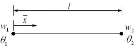
₍₇₎

where x_i is the location of the left edge of the element

i and x_N+1 = R is the radius of the beam. Consider the two noded, 4 degree of freedom beam finite element shown in Fig. 1. The boundary conditions for the element of length l are given by w(0) = w₁,

1 2

(0)

, dw

w

dx   w(l) = w3, 2 4

( )

. dw l

w dx  

Putting Eq. (6) into the element boundary conditions

yields:

w

₁

  

a

₀

a

₂

a

₃

,

w

₂

 

a

₁

Ca

₂



Ca

₃

,

3

w

=

a

0



a l

1 + 2

Cl

a e +a e₃ Cl and

w

4=

a

1– 2

Cl

a Ce +a Ce₃ Cl. Here we have dropped the subscript i in C as the entire discussion here is relevant

within the finite element. Solving for

a a a

₀

,

₁

,

₂ and

a₃ in terms of the nodal displacements and slopes using the above expressions, w can be approximated by

1 1 2 2 3 3 4 4

w



w N



w N



w N



w N

(8)

where

N N N

₁

,

₂

,

₃ and

N

₄ are the stiff-string shape functions and are given as

 

1 2

3 4

, ,

,

R x R x

N N

D CD

R x R x

N N

D CD

 

  (9)

[image:2.612.324.543.411.492.2]

(3)

where

4 2 Cl 2 Cl Cl Cl

D   e  e Cle Cle

 

1 2

Cl Cl Cl

Cx Cl Cx Cx Cx Cl

e e Cle

R x Cle Cxe Cxe

e e e e

 



   

    

 

 _    _

_ _ _ _ 

 

 

2

Cl Cl Cl Cl

Cl Cl

Cx Cl Cx Cl

Cx Cx Cl Cx Cl Cx

e e Cle Cle

Cxe Cxe Cx

R x

e Cle

e e Cle e

 



   

  

    

_ _ _ 

 

_ _

  

 

 _ _ _ 

 

 

3

2

Cl Cl Cl

Cl Cx Cl Cx Cx Cx Cl

e e Cxe

R x Cxe e e

e e

 

   

    

 

 _   _

_ _ 

 

 

4

2 Cl Cl 2

Cl Cl Cx

Cx Cx Cl Cx Cx Cx Cl

Cl e e Cx

Cxe Cxe Cle

R x

e e e

Cle e



 

   

    

_ _ _ 

 

_ _

  

 

_ _ 

 

(10)

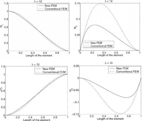
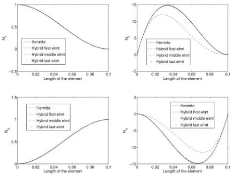
These shape functions are called the stiff-string shape functions. Fig. 2 compared these stiff-string

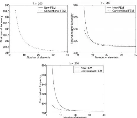
shape functions with the conventional Hermite cubics for one element case and with a non-dimensional rotational speed of 12. Fig. 3 shows this comparison at a much higher rotation speed. Figs. 4 and 5 clearly show the good performance of the stiff-string basis functions, especially for the important fundamental mode. This effect if more significant at the higher rotation speed. Table 1 and Table 2 show the comparison of predictions of rotating beam frequencies with the published literature. It can be observed that the stiff-string basis function depend

Fig. 2: Variation of shape functions along the elements (N = 1,= 12) with the new and conventional finite element at high rotation speed

Fig. 3: Variation of shape functions along the elements (N = 1, = 200) with the new and conventional finite element at very high rotation speed

[image:3.612.317.548.82.277.2] [image:3.612.67.295.509.702.2] [image:3.612.318.548.519.721.2]

(4)

on the material property of the element and on the local tension level. Thus, these shape functions adjust to the physics of the problem.

The analytical limits of these stiff string basis functions as the rotation speed tends to zero is shown in Eq. (11) to become the Hermite cubics.

3 2 3 3 2 2

1 3 2 2

0 0

2

3

2 lim

, lim

C C

x

x l

l

x

x l

xl

N

l

 











3 2 3 2

3 3 4 2

0 0

2

3 lim

, lim

C C

x

x l

x

x l

N

l

 









(11)

As the rotation speed tends to infinity, the interpolation functions and become linear and approach zero, as given in Eq. (12).

1 2

3 4

lim 1 , lim 0,

lim , lim 0

C C

x

N N

l x

N N

l

 

  

  (12)

In a following work, Gunda et al proposed the hybrid stiff-string polynomial basis functions (Gunda

et al., 2009),

2 3

0 1 2 3

4 5

( )

Cx Cx

w x

a

a x

a e



a e

 



(13)

The idea here is to keep the cubic polynomial which works well for the non-rotating beam and add the stiff string basis which works well for beams at high rotating speeds. These hybrid shape functions were obtained by adding a centre node with displacement and slope degrees of freedom to the finite element as shown in Fig. 6. This additional node with two degrees of freedom allows us to determine all the six constants in Eq. (13). The expressions for the shape functions are given in Reference (Gunda

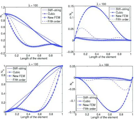
et al., 2009). Fig. 7 and 8 show the new hybrid basis

functions, along with stiff string, Hermite cubic and fifth order polynomial basis functions. Fig. 7 results are for an element at low rotation speed of  = 12 and Fig. 8 shows results for an element at high rotation speed of = 100. The new basis functions adapt to rotation speed changes. Fig. 9 shows the mode shapes of the cantilever beam. It can be observed that at high rotation speeds, the beam behaves like a rotating cord. The hybrid stiff-string polynomial basis functions

Fig. 5: Convergence of the natural frequencies with  = 200

Fig. 6: Beam finite element with centre node for hybrid stiff-string polynomial basis functions

(5)

[image:5.612.68.296.81.284.2]

Fig. 8: Variation of shape functions (N = 1,= 100) with the new, stiff-string, conventional cubic and fifth order finite elements

Table 1: Comparison of non-dimensional natural frequencies of cantilever uniform beam

Mode Present- Wang and Wright Hodges FEM Wereley et al. et al.

 = 12

[image:5.612.319.546.82.185.2]

1 13.1702 13.1702 13.1702 13.1702 2 37.6031 37.6031 37.6031 37.6031 3 79.6145 79.6145 79.6145 79.6145 4 140.534 140.534 140.534 N/A 5 220.537 220.537 220.537 N/A

Table 2: Comparison of non-dimensional natural frequencies of hinged uniform beam

Mode Present- Wang and Wright FEM Wereley et al.

 = 12

1 12.0000 12.0000 12.0000 2 33.7603 33.7603 33.7603 3 70.8373 70.8373 70.8373 4 126.431 126.431 126.431 5 201.123 201.122 201.122

addressed the issues of convergence of the stiff string basis functions which favoured the fundamental node and did not give good results for higher nodes. The hybrid basis functions performed well for all modes.

Physics Based Basis Function

Consider the static homogenous equation of the rotating beam rewritten as,





4 2

2 2

4

0

2 d w

m

d

dw

EI

R

x

dx









_

_



_

_



(14)

Let

2 4

2

m

L

EI







Then,





4 2

2 2

4 4

0

2 d w

d

dw

L

x

dx

L dx

dx









_

_



_

_



(15)

We split the above equation into two parts and find their solution [15],

4

0 d w

dx



(16)



2 2



0

d dw

L x

dx dx

 _ _

 

  (17)

This yields two equations as solutions of Eq (16) and Eq. (17),

(1) 2 3

0 1 2 3

W a a xa x a x (18)

(2)

ln L x

W a

L x 

 

 __ __

 (19)

The basis function used to create finite element shape functions is thus,

[image:5.612.338.547.306.435.2] [image:5.612.66.294.541.662.2]

(6)

(1) (2)

0 1

2 3

2 3 4

( )

ln

w x

W

a

a x

L

x

a x

a

L

x





 









_

_

_

_



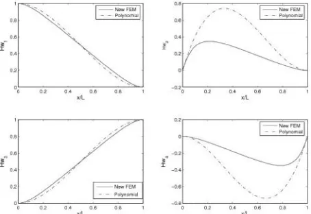
(20)

Ganesh and Ganguli (2013) developed this approach and found that this approach worked well for rotating beams. The additional constant is addressed by forcing the error given by the basis function to zero at the element midpoint. The complete shape functions are given in Ref. Ganesh and Ganguli (2013). Figs. 10 and 11 show the shape functions. The difference between the polynomial and these physics based functions is amplified at higher rotation speeds.

Point Collocation Method

Here, we write the static homogenous equation as,

4 2 2 2 2 2 2

4 2 2

2

0 d w

m

R d w

m

x d w

dx

EI

dx

EI

dx

m

x dw

EI

dx













(21)

Let,

2

m

c

EI





and 2 2

2 m

L

d

EI





4 2 2 2

4 2 2

0

2 d w

d w

cx d w

dw

d

cx

dx



dx



dx



dx



(22)

The cubic polynomial does not satisfy Eq. (22). Consider a collocation point located inside the finite element and choose a basis function as,

2 3 4

0 1 2 3 4

wa a xa x a x a x (23)

Now, the interpolating polynomial is required to satisfy the ODE at x. This yields a₄ in terms of

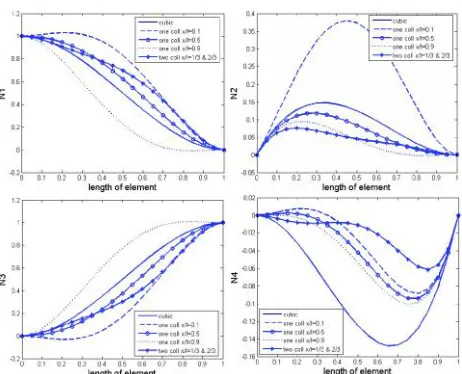
a₀, a₁, a₂ and a₃. These collocation inspired basis functions are used to get shape functions by Sushma and Ganguli (2012). Fig. 12 and 13 show the shape functions.

Rotor Blade Problem

A rotor blade can be modelled as a beam with axial (u_e), lag bending (v), flap bending (w) and torsion

Fig. 10: Comparison of shape function values for  = 12 for different elements in the beam

Fig. 11: Comparison of shape function values for = 100 for different elements in the beam

(7)

degrees () of freedom. A simplified model with these motions can be written as



2 

0

e e e

EAu





m x u

  

v u

 



(24)

2

0

l IV

Z e

x

EI v

mv

mu

v

mxd















_



_













(25)

0

l IV

y

x

EI w

mw

w

mxd













_



_











(26)



2 1



2 2 2

0

m m m

GJ







mK







m



K



K



(27)

Here EA is the axial stiffness, EI_z is the inplane or lag bending stiffness, EI_y is the out-of-plane or flap bending stiffness and GJ is the torsion stiffness. Also

2

m

K is the radius of gyration.

To derive the shape functions based on the logic discussed in the previous sections, we remove the inertial and velocity terms to obtain the static part of the governing homogenous differential equations. These equations in dimensional form are given as:

2

0

e e

EAu m u  (28)

2 2

0

L IV Z x

EI v

m

v

m

xd









  

_





_









(29)

2

0

L IV y x

EI w

w

m

xd











_





_









(30)



2 1



2 2 2

0

m m

GJ





 

m



K



K



(31)

where,

2

L x

T 



m xd ₍₃₂₎

The constant tension T_i for the element is approximated by taking the average centrifugal tension in the element. The centrifugal tension T_i for the ith_{element can be expressed as:}

2

i

L

i i

x

T





m



xdx

₍₃₃₎

Here x_i is the location of the left edge of the finite element. The solutions of the differential equations (28) to (31) are obtained as:

2 2

1

sin

2

cos

e

m

u

C

x

C

x

EA



_





_





_

_



_

_









(34)

2 2 3 2 2 4 2 2 5 2 2 6

4 exp

2

4 exp

2

4 exp

2

4 exp

2

Z Z Z Z Z Z Z Z

T

EI m

C

x

EI

T

EI m

C

x

EI

v

T

EI m

C

x

EI

T

EI m

C

x

EI





_

_

_





















_

_









_

_











_

_

_





_

_











 

_

_





_





_









_

_





_

_













_

_









_























(35)

7 8 9

10

exp

y y

T

w

C

C x C

x

EI

T

C

x

EI









































(36)

[image:7.612.68.299.79.266.2]

(8)









2 1

2 2 2

11

2 2 2

12

exp

m m

m K K

C x

GJ

m K K

C x

GJ

     

 

 

 _ _ 

 

 

 

 

(37)

These solutions were used to obtain shape functions for a rotor blade by Chhabra and Ganguli (2010). Figs. 14-16 show these shape functions along with the classical polynomials. Again, these shape functions give better results at high rotation speeds, relative to the polynomials. The shape functions contain the material properties and rotation speed of the blade, allowing them to adapt to different rotation speeds and non-uniform geometries.

Spectral Finite Element Method

The spectral finite element method solves the free vibration problem in the frequency domain. We construct the weak form of the governing differential equation and write the total energy of a non-conservative rotating system in transverse motion is the frequency domain as,

 

2

2 2 0

2

0 1

2 2 0

2 0

1 ( )

2

1 ( )

2

1 ( )

2

1 _ˆ

2

n

L

n L

n N

i t

L n

n n L

T n n

d w

E I x

dx

dw

T x

dx

e

A x

w dx

i

w dx

F

W







 





_

_





_

_

_

_

















_

_

_











 

_

_



_

_















 







_{ }



















(38)

where

ˆ

,

 

T

F

W

 

 



represents the externally applied nodal force and nodal displacement vectors in frequency domain,_n the circular frequency of the

th

n

sampling point, andw_n is the spatially dependent Fourier coefficient and  is the damping force per

Fig. 14: Shape functions in flapwise bending at 383rpm

Fig. 15: Shape functions in lead-lag bending at 383

Fig. 16: Shape functions in axial deformation and torsion at 383 rpm

unit length, per unit velocity. According to principle of minimum potential energy in the frequency domain,

(9)

i.e.,

 

 

2 2 2 2 0 0 2 0 0 ( ) ( ) 0 ( ) ˆ L n n L n n L

n n n

L

T

n n n

d w d

E I x w dx

dx dx

dw d

T x w dx

dx dx

A x w w dx

i w w dx W F

                _ _    _ _   _{ }   _ _      _ _ _{ }       



 _  _      (39)

To obtain the dynamic stiffness matrix in frequency domain, we need to substitute an interpolating function for the transverse displacement

 

w

n



in Eq. (39). We consider two choices for the

interpolating function and hence two types of elements viz: the SFER and SFEN are formulated.

Interpolating Function for SFER

To obtain the interpolating function for SFER, we assume the beam to be uniform and replace T(x) by the maximum centrifugal force, T_max (Thakkar and Ganguli, 2006). 2 2 2 max 0 ( ) 2 L A L

T 



A x  xdx   ₍₄₀₎

This allows us to represent of the rotating beam with damping, as a constant coefficient PDE, which can be written as

4 2 2

max

4 2 2

0 w

w

EI

T

A

x



t



t



_



_



_



_



(41)

where is the damping force per unit length, per unit velocity. Eq. (41) is analogous to the “stiff string’’ equation where the tension is constant along the length. The exact solution of this equation, in frequency domain is given as

   

1 4

2 3

1 2

3 4

ˆ ( ) n n

n n

ik x ik x

n n n

ik L x ik L x

n n

w x C e C e

C e C e

 

  



where k_pn is the wave number, obtained from the relation.

2

2 2 2 2

4 2 2 2 n n pn i A

A L A L

EI EI EI EI

k                                 (42)

Here, p represents the modes of wave propagation. Eq. (42) is the interpolating function for SFER in the frequency domain.

Interpolating Function for SFEN

Similar to SFER, we can obtain the interpolating function for SFEN by assuming the beam to be uniform and non-rotating. This can be obtained by substituting

T_max = 0 in the rotating beam equation, which then reduces to the form

4 2

0 w

w

EI

A

x



t



t



_



_



_



(43)

The exact solution of Eq. (43) is given by

   

1 4

2 3

1 2

3 4

ˆ ( ) n n

n n

ik x ik x

n n n

ik L x ik L x

n n

w x C e C e

C e C e

 

 

  (44)

But here, the wave number is different from the previous case and is given by

2 n n pn A i k EI EI      _{ }     __ _{ }_{ } ___  

  (45)

Where p represents the mode of wave propagation. Eq. (45) is the frequency domain interpolating function for SFEN. Vinod et al showed the advantages of using the spectral finite element method for rotating beams (Thakkar and Ganguli, 2006; Vinod et al., 2007). To compare the spectral finite element methods, the resonant peaks for a uniform cantilever beam and a hinged beam are compared in Fig. 17.

(10)

2 2

( , ) ( , )

( ) ( ) ( , )

( , )

( ) 0

x t w x t

I x GA x k x t

t x

x t EI x

x x



 



 _  _ 

 

 

 

   

 __ __

 

(47)

where T(x) is axial force due to centrifugal stiffening and is given by

2

( ) ( )

L x

T x 



A x  dx

Here L is the length of beam, is the rotational speed,(x, t) is angle of rotation of cross section,

w(x, t) is the vertical displacement of beam, is the density, E and G are elastic constants, k is the shear coefficient, A(x) is area of cross section, I(x) is moment of inertia of cross section. The

non-dimensional constants are

2

,

AL

I





GAkL

2

EI





and Gk,

E  



  2 2 4

.

A

L

k

EI







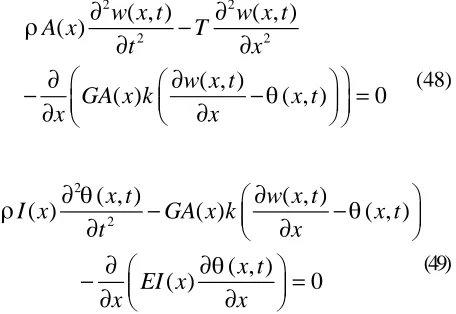
For beams with

constant tension, Eqs. (46) and (47) reduce to

2 2

( , ) ( , )

( )

( , )

( ) ( , ) 0

w x t w x t

A x T

t x

w x t

GA x k x t

x x





 _ 

 

   

 _ __  ___

 

 

(48)

2 2

( , ) ( , )

( ) ( ) ( , )

( , )

( ) 0

x t w x t

I x GA x k x t

t x

x t EI x

x x



 



 _  _ 

 

 

 

   

 __ __

 

(49)

where T is the constant axial tension. We call these the violin string equations in an analogy to the typical Euler-Bernoulli stiff string equations. The stiff strings are studied in the acoustic analysis of piano strings. Piano strings have flexural stiffness but are typically quite long. In fact, the most prized pianos are those with the largest strings. Violins are much smaller than pianos. Timoshenko theory gives a better representation of inharmonicity of violin strings

[image:10.612.68.298.80.308.2]

Fig. 17: (A) and (B) Resonant peaks of uniform cantilever beam, (C) and (D) Resonant peaks of uniform hinged b e a m

Table 3: Convergence study on the natural frequencies of uniform beam for = 12, using the spectral elements SFER (rotating beam basis functions assuming constant (maximum) centrifugal force) and SFEN (non-rotating beam basis functions)

Mode SFER SFEN SFER SFEN Exact

n = 8 n = 16

1 13.1731 13.1731 13.1731 13.1731 13.1702 2 37.6017 37.6113 37.6017 37.6017 37.6031 3 79.6136 79.6328 79.6136 79.6136 79.6145 4 140.5318 140.5702 140.5318 140.5318 140.5342 5 220.5385 220.6056 220.5385 220.5385 220.536

but the difference in predicted frequencies is small.

Violin String Basis Function

The earlier examples considered Euler-Bernoulli rotating beams. However, short beams are better modelled as Timoshenko beams. The governing equation for free vibrations of a rotating Timoshenko beam is given by (Vinod Kumar and Ganguli, 2012).

2 2

( , )

( )

( , )

( )

( , )

0 w x t

w x t

A x

T x

t

x

w x t

GA x k

x t

x







_



















 









_

_



_

_

_









(46)

(A) (B)

[image:10.612.320.548.445.602.2]

(11)

compared to Euler-Bernoulli beam theory (Maezawa

et al., 1988). The static part of Eqs. (48) and (49) is

obtained by ignoring the inertial term which leads to

2

( )

0 d w

d

dw

T

GA x k

dx









_

_



_

_

_







(50)

( ) dw d ( )d 0

GA x k EI x

dx dx dx

 

 _ _  _

   

    (51)

Putting Eq. (51) in Eq. (50) yields and putting T = 0 for a non-rotating beam.

2

( )

0 d

d

EI x

dx





_{ }









(52)

For a uniform beam,

 

3

2

0 1 2

3

0 d

x

a

a x

dx



_{ }

_

_{ }

_

(53)

Also, for a uniform beam, Eq. (52) and Eq. (53) give

2 2

d w

d

dx





(54)

2

0 dw

EI d

dx

GAk dx



 



(55)

We see that the typical cubic shape functions used for the displacement field w(x) satisfies the non-rotating Timoshenko beam equation. It therefore works quite well for a non-rotating beam. Friedman and Kosmatka (1993) also ensured that the w(x) and

(x) displacement fields satisfied both Eq. (52) and Eq. (53) for a uniform beam. In the case of axially loaded beams, Kosmatka used the same shape functions and did not include the axial force. This yields

2 3

1 2

3 0 2

2 ( )

2 3

a a

EI

w x a a a x x x

GAk

 

 __  __   ₍₅₆₎

as the displacement field. We see that four constants

a₀, a₁, a₂ and a₃are present in w(x) and(x) which can be calculated from four nodal values for an element.

We propose to use Eqs. (50) and (51) to derive new shape functions which are suitable for rotating Timoshenko beams. The presence of T(x) in Eq. (1) presents a difficulty in obtaining an analytical solution. While the assumption of T(x) = T = constant may appear too simplistic for the whole beam, it is reasonable if the beam is divided into several finite elements and T is assumed constant within each element. Thus, the rotating beam is assumed as a sequence of violin strings for the calculation of shape functions.

Using the finite element method, the beam is divided into N number of elements of equal length. The tension T(x) is assumed as constant T_iwithin the element i, which reduces the rotating beam equation to the violin string equation. For an th

i

element along the beam, the relationship between global and local coordinates is given by

i

x

 

x

(57)

where x_i = (i – 1)l is the distance from the root to the

left edge of element i, l is length of the element and

x is the local element coordinate.

 

1

2

( ) ( )

j

L i

x x j N

j j i _x

T x T A x xdx

m x xd x 



 

  

 



 

(58)

The tension in the inboard elements is high and decreases for the outboard elements. Assuming EI(x) = EI_i andA(x) =A_i within an element as constant, we get

2 2

0

i

d w

d

T

GAk

dx









_



_











(59)

2

2 0

dw d

GAk EI

dx dx



  

 _ _ _

   

    (60)

This yields

3 2

i

T

d

d w

dx

EI dx



_

(12)

Note that this equation relates(x) and w(x) is quite different from Eq. (53). Also, if T_i = 0, Eq. (61) yields Eq. (53) for the non-rotating beam. We remove the coupling between w and to yield,

4

0

1

i i i

i

T

d w

d

dx

T

dx

EI

GA k



















(62)

3

0

1

i i i

i

T

d

dx

T

dx

EI

GA k



_



_















(63)

The solutions of which are

 

0 1 2

dx dx

x b b e b e

 _{ }  _ ₍₆₄₎

where





2 2

3

1 1

i i i

i

T C

d

C m T

EI

GA k

 

 _  

 

 

and

,

3

.

i i

T

EI

C

m

EI

GA k



The displacement field w(x) is given by

 





















0

2

1 2 3

3

2

2 2 3

3

0 2

3

1

dx

b x

e

b

x

C m

d

C m

w x

e

b

x

C m

d

C m

a

C m











_{ }

_{ }

_







_

_{ }

_{ }





_





















_



 

_

_





 







_

_

_{ }

_



















_







(65)

where,





2

3 2

3

1

1 1

m d

C m

   

 .

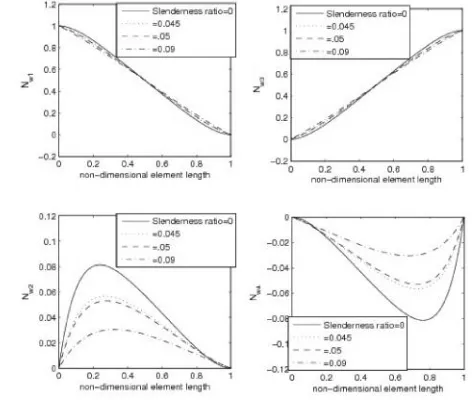
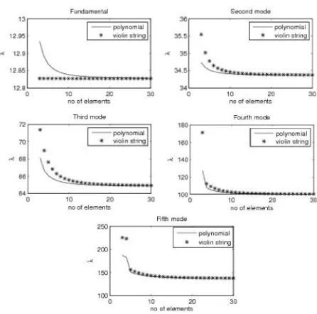
This displacement function satisfies the static homogeneous violin string equations within the element and is used to create the violin string shape functions (Vinod and Ganguli, 2011). Fig. 19 and 20 show the displacement and rotation shape functions. Fig. 21 shows the convergence of the first five modes using polynomial and violin string basis functions.

Fig. 18: Timoshenko Beam Element

Fig. 19: Displacement shape functions at different slenderness ratios for K = 12

(13)

Concluding Remarks

This paper reviews some research on the development of physics based shape functions for the finite element analysis of rotating beams. The rotating beam

differential equation has two extreme limits. The first case is when the rotation speed is zero, which is the non-rotating beam. The other case is a beam rotating with very high speed, in which case the centrifugal stiffness can exceed the flexural stiffness and the beam behaves like a rotating cord or string. Various approaches to develop new shape functions were illustrated in this paper. These shape functions yield better convergence at high rotation speeds. Fast convergence also allows the creation of low order finite element models which are useful for control applications. The possibility of using spectral finite element methods for the rotating beam problem is also discussed. Furthermore, a novel approach to enrich shape functions by requiring them to satisfy the governing differential equation at selected points in the element is presented. It is also found that the rotating beam problem can be used as a pedagogical tool to illustrate the finite element method to students in engineering sciences.

Acknowledgements

The author acknowledges his former students J B Gunda, K G Vinod, R Ganesh, P Sushma, P P S Chhabra and A S Vinod Kumar for their help in doing the research discussed in this paper.

Fig. 21: Convergence of first five modes for slenderness ratio 1

.05

  at K = 12

References

Wang G and Wereley N M (2004) Free vibration analysis of rotating blades with uniform tapers AIAA Journal 42 2429-2437

Ganguli R, Chopra I and Weller W H (1998) Comparison of calculated vibratory rotor hub loads with experimental data Journal of the American Helicopter Society 43 312-318

Banerjee J R (2000) Free vibration of centrifugally stiffened uniform and tapered beams using the dynamic stiffness method Journal of Sound and Vibration 233 857-875 Bokaian A (1990) Natural frequencies of beams under tensile

axial loads Journal of Sound and Vibration 142 481-498 Wright A D et al. (1982) Vibration modes of centrifugally stiffened

beams Journal of Applied Mechanics 49 197-202 Cai G P, Hong J Z and Yang S X (2004) Model study and active

control of a rotating flexible cantilever beam International

Journal of Mechanical Sciences 46 871-889

Banerjee J R (2001) Dynamic stiffness formulation and free

vibration analysis of centrifugally stiffened Timoshenko beams Journal of Sound and Vibration 247 97-115 Lee J W and Lee J Y (2016) Free vibration analysis using the

transfer-matrix method on a tapered beam Journal of Sound

and Vibration 164 75-82

Huo Y and Wang Z (2015) Dynamic analysis of a rotating double-tapered cantilever Timoshenko beam Archive of Applied

Mechanics 1-15

Du H, Lim M K and K M Liew (1994) A power series solution for vibration of a rotating Timoshenko beam Journal of

Sound and Vibration 175 505-523

Meirovitch L Fundamentals of Vibrations Waveland Press 2010 Banerjee J R (2000) Free vibration of centrifugally stiffened uniform and tapered beams using the dynamic stiffness method Journal of Sound and Vibration 233 857-875 Gunda J B and Ganguli R (2008) Stiff-string basis functions for

vibration analysis of high speed rotating beams Journal of

Applied Mechanics 75 024-502

[image:13.612.69.292.79.300.2]

(14)

stiff-string-polynomial basis functions for vibration analysis of high speed rotating beams Computers & Structures 87 254-265 R Ganesh and R Ganguli (2013) Stiff string approximations in Rayleigh-Ritz method for rotating beams (2013) Applied

Mathematics and Computation 219 9282-9295

D Sushma and R Ganguli (2012) A collocation approach for finite element basis functions for euler-bernoulli beams undergoing rotation and transverse bending vibration

International Journal for Computational Methods in Engineering Science and Mechanics 13 290-307

Chhabra P P S and Ganguli R (2010) Superconvergent finite element for coupled torsional-flexural-axial vibration analysis of rotating blades International Journal for

Computational Methods in Engineering Science and Mechanics 11 48-69

Thakkar D and Ganguli R (2006) Use of single crystal and soft piezoceramics for alleviation of flow separation induced vibration in a smart helicopter rotor Smart Materials and

Structures 15 331

Vinod K G, Gopalakrishnan S and Ganguli R (2007) Free vibration

and wave propagation analysis of uniform and tapered rotating beams using spectrally formulated finite elements

International Journal of Solids and Structures 44

5875-5893

Vinod Kumar A S and Ganguli R (2012) Analogy between Rotating Euler-Bernoulli and Timoshenko beams and stiff strings

Computer Modeling in Engineering & Sciences(CMES) 88

443-474

Maezawa S, Temma K and Ochai H (1988) Vibration of a bowed

string. Application of Timoshenko’s beam theory and

transmission of sound energy through the bridge JSME

International Journal 3 Vibration, control engineering,