Applying a reverse design modelling technique to partial core transformers

APPLYING REVERSE DESIGN MODELLING TECHNIQUE TO PARTIAL CORE TRANSFORMERS

M.C. Liew and P.S. Bodger

Department of Electrical and Electronic Engineering University of Canterbury

Abstract

This paper gives an overview of the process of designing partial core transformers using a reverse modelling technique. Modifications are made to full-core equivalent circuit components to accommodate partial core transformers. The model is applied to 50Hz transformers under normal operating temperature applications and also to transformers immersed in liquid nitrogen. It is then used for harmonic frequency analysis of partial core transformers where capacitive components are included. In all cases, comparisons are made between the model calculations and test results of as-built devices.

1. INTRODUCTION

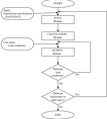
There are limitations to the conventional approach to transformer design. The terminal voltages, VA rating and frequency are input specifications and determine the types and dimensions of materials to be used. Core and winding material characteristics are known from standard values or physical measurements. The resultant design may not match what is actually available in materials and hence the predicted performance can be in error. A reverse design method has been presented [1,2], whereby the physical characteristics and dimensions of the windings and core are the specifications. By manipulating the amount and type of material actually to be used in the transformer construction, its performance can be determined. Fig. 1 shows the flow diagram of the reverse design method.

START

DATA Module

END OUTPUT Module CALCULATION Module

Different load conditions? User input:

Load conditions Input:

Transformer specifications (DATA.DAT)

Yes

No

Different transformer or

input specs? Yes

No

Fig. 1. Reverse transformer design flow chart

In this paper the reverse design method is applied to partial core transformers. Modifications are made to the equivalent circuit components of full-core transformers to model partial core transformers. The model is validated under normal operating conditions. The accuracy of this new partial core model is then tested for transformers under liquid nitrogen (N2)

[image:1.595.78.282.502.729.2]

conditions. The measured results are compared to model calculated values. Finally, harmonic frequency analysis of the partial core transformers is performed. Necessary alterations are made to the calculation of the equivalent circuit parameters. Capacitive components are added into the reverse design partial core model, as the effect of these stray capacitances can no longer be neglected at high frequencies. 2. PARTIAL CORE TRANSFORMERS

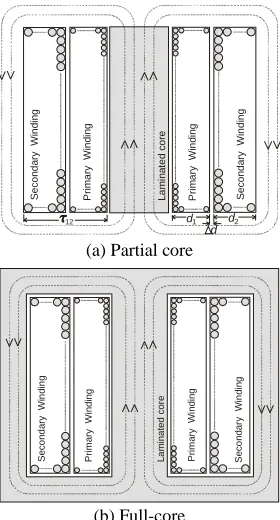
Fig. 2a shows a cross-sectional view of a partial core transformer. The laminated core occupies the central space. The windings are wrapped around the core. The yokes and limbs, which usually form the rest of the core in full-core transformers (see Fig. 2b), are not present. Therefore, the performance of these transformers is expected to be different. Partial core transformers are being studied because of their potential use with superconducting windings where the size of the core can be dramatically reduced albeit by an increase in winding turns. The combination means that the overall weight of the partial core units is significantly reduced, and they are easier to manufacture.

P rim ar y W ind in g S e c o n d a ry W indi ng P ri m ar y W ind in g S e c o nd ar y W in d in g La m inat e d c o re d

12 d1 d2

(a) Partial core

[image:2.595.309.523.82.355.2]

P ri m ary W indi ng S e c o ndar y W in d in g P ri m ary W indi ng S e c o nd ary W in d in g La mi na ted c o re (b) Full-core

Fig. 2. Transformer’s cross-sectional views

Consideration is given to the transformer equivalent circuit shown in Fig. 3, where capacitances have been included for the harmonic analysis in the later section.

R1 XC1 XC12 V1 + -V2 -+ Rh Rec Xm X2

X1 R2

,

, ,

[image:2.595.111.251.85.345.2]

XC2 H

Fig. 3. Transformer equivalent circuit

For the core components, the partial core magnetising reactance is derived in the previous work [4]:

core core rT o m l A N

X ω µ µ

2 1

= (1)

where N1 = number of primary winding turns Acore = cross-sectional area of the core µo = 4π× 10-7 Hm-1

µrT = transformer overall permeability

lcore = length of the core ω = 2πf

µrT is obtained by taking into account the magnetic

flux generated by the energised winding which flows through the core and returns via the air, back to the core. Approximations to the distribution of the flux within partial core transformers with different winding thickness factors are depicted in Fig. 4.

lcore Pri m ary S e c o nd ar y Pri m ary S e c o nd ar y 1

(a) Winding thickness factor τ1

lcore Pr im ar y Pr im ar y S e c o nd ar y 2 S e c o nd ar y

(b) Winding thickness factor τ2

Fig. 4. Flux distribution within the partial core transformer

with different winding thickness factors

The two transformers have the same core length. The flux path is uniform within each core. The air flux path is dependent on the winding thickness factor τ. For a partial core transformer with a smaller thickness factor,τ1, the flux flows through a relatively shorter air

path (Fig. 4a) compared to the one with a larger thickness factor τ2 (Fig. 4b). Therefore, the aspect

ratio of the transformer affects the air flux path and hence the overall relative permeability and the magnetising reactance of the partial core transformer. Thus: core T o core a rT A l ℜ Υ = µ β

µ ( ) (2)

where

ℜ

_T = transformer overall reluctance 12 τ β core a l =

Υ(βa) is the magnetising function, expressed as a function of the transformer aspect ratio βa [5]:

   ₋ − = Υ ς β β a

a) 1 exp

( (3)

ς determines the rate of saturation of the function.

[image:2.595.72.286.415.507.2]

air

R

air

R

core

R mmf

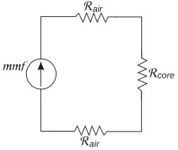
Fig. 5. Magnetic circuit of the transformer

The overall reluctance is thus:

air core

T =ℜ + ℜ

ℜ 2 (4)

where

ℜ

_core = core reluctance

ℜ

_air = air path reluctance

When calculating the total core loss resistance of the partial core transformer, both the eddy current loss and the hysteresis loss components are taken into account [6]. The hysteresis loss for a partial core transformer is [4]:

x core

hpc k fB

P =υ1+α α ₍₅₎

h R e2

= (6)

where υ = volume of the core

Bcore = maximum core flux density

k = partial core hysteresis loss constant α = partial core factor

x = Steinmetz factor

By substituting (5) into (6), the hysteresis loss resistance Rh can be calculated. Next, the eddy current

resistance Rec is expressed as [7]:

c l

A N

R core

core core ec

ρ

12 2 1

= (7)

where ρcore = operating resistivity of the core

c = core lamination thickness

Rh and Rec are in parallel, thus forming the total core

resistance Rcore.

The total leakage reactance (X1 + X2’) of a partial core

transformer is calculated from [4]:

core o a leak

l N

X ( ) 4 12 ’

2 1 τ δ

ωµ β

Γ

= (8)

where τ12

2

1 d d

d +∆ +

= (see Fig. 2a)

₌d +d _+∆d 3

’ 1 2

δ

Γ(βa) is the leakage function, expressed as a function of the transformer aspect ratio βa:

  

₋

− = Γ

ζ β

β a

a) 1 exp

( (9)

ζ determines the rate of saturation of the function.

Finally, The primary and secondary winding resistances R1 and R2’ can be calculated using the

general form [1]:

A l

R=ρ (10)

where ρ = operating resistivity of the conductor

l = effective length of the wire A = cross-sectional area of the wire

Under short circuit conditions, they are combined to form Rwinding.

[image:3.595.118.244.85.191.2]

Sample transformers have been built and tested under normal temperature conditions to determine the equivalent circuit parameters derived. Another transformer was designed, built and tested to verify the component models. This is shown in Table I.

TABLE I

Calculated and measured test results under normal operating temperatures

Parameters Normal Temperature Equivalent Circuit Calculated Measured Error(%)

Rcore (Ω) 522 551 5

Xm (Ω) 42.0 42.6 1

Rwinding (Ω) 3.7 3.5 6

Xleak (Ω) 4.5 4.6 3

Performance Calculated Measured Error(%)

V1 (V) 234 234 0

I1 (A) 23 23 0

V2 (V) 21 25 16

I2 (A) 112 109 3

P1 (W) 4.4 4.2 5

Effy. (%) 56 60 7

Reg. (%) 53 51 4

Significant agreement has been achieved between the values of the transformer equivalent circuit components as determined through calculation and test. In addition, calculated and measured operational performances also show good agreement.

3. LOW TEMPERATURE OPERATION

temperature. In [1], the operating resistivity at temperature T°C is given as:

(

)

(

ρ

)

ρ ρ ρ

∆ + ∆ + =

20 1 1

20 C

T o ₍₁₁₎

where ∆ρ = thermal resistivity coefficient

ρ20°C = material resistivity at 20°C

It was found that the operating resistivity value of the copper conductor produced erroneous calculation at extremely low temperatures. Therefore, Equation (11) needs to be modified to account for the difference at extremely low temperatures.

The new resistivity calculation for the copper conductor, which takes into account the low temperature effects, is:

8 11

10 57 . 1 10 99 .

6 × − + × −

= T

ρ (12)

It has been validated for the operating temperatures of the copper conductor between 70°K (-203°C) and 400°K (127°C) [8].

Consider the current distribution in the cross-section of a cylindrical conductor shown in Fig. 6.

w

2

w

w

2

ec w

(a) 2

w ec >

δ (b) 2

w ec < δ

Fig. 6. Current distribution in the conductor due to skin

effect

The skin depth is defined as [9]:

ω µ

µ ρ

δ

r o ec

2

= (13)

where µr = relative permeability of the material When the skin depth is significantly greater than half the conductor thickness, the AC current flowing in the conductor is uniformly distributed within the diameter of the conductor. This is illustrated in Fig. 6a.

However, as the frequency increases, the skin depth drops. At some stage the skin depth drops below half the conductor thickness. As a result, the current distribution within the conductors is no longer

uniform. The current concentrates towards the outside surfaces of the conductor. The effective current carrying cross-sectional area can be seen in Fig. 6b. In reality the current distribution in a semi-infinite conductor decays from the surface value exponentially. The skin depth in Fig. 6b is an approximation of this. The effective cross-sectional area of the winding conductors thus becomes [5]:

2 2

2 2

2 _

 

  − −      

= w w ec

A π π δ

=πδ_ec(w−δ_ec) (14)

For the hysteresis loss resistance defined in Equation (5), the flux density Bcore is calculated as:

core core

A N

V B

1 1 2

ω

= (15)

where V1 = input voltage

Since the effective cross-sectional area of the core is made up of laminations, and these laminations are affected by the skin depth, the area Acore in which the

flux flows is replace a new effective area [8]:

_{( 2 )( 2 )}

ec core ec core core core

core b w b w n

A = − − δ − δ (16)

where bcore = breadth of the core wcore = width of the core

n = number of laminations

The eddy current resistance Rec is also affected by the

skin depth. The new eddy current resistance of the core, taking into account the skin depth, is:

  

 + −

=

ec

ec core core

core core ec

n w nb l

N R

δ

δ

ρ 2

2 2

1 (17)

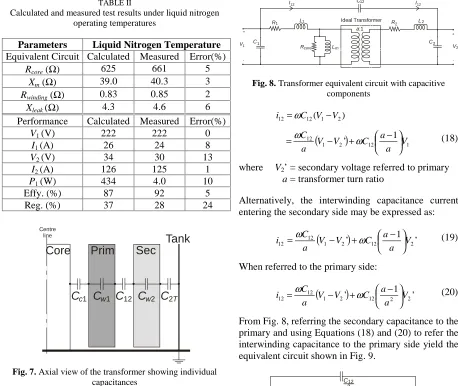
Sample transformers were designed, built and tested. From the results obtained, modifications were made to the resistance parameters of the reverse design model to account for the changes in the resistance of the materials at very low temperatures. Another transformer was then designed, built and tested to verify the component models. This is shown in Table II. Again, significant agreement has been achieved between test results and calculated values.

4. HIGH FREQUENCY ANALYSIS

[image:5.595.66.524.87.473.2]

TABLE II

Calculated and measured test results under liquid nitrogen operating temperatures

Parameters Liquid Nitrogen Temperature Equivalent Circuit Calculated Measured Error(%)

Rcore (Ω) 625 661 5

Xm (Ω) 39.0 40.3 3

Rwinding (Ω) 0.83 0.85 2

Xleak (Ω) 4.3 4.6 6

Performance Calculated Measured Error(%)

V1 (V) 222 222 0

I1 (A) 26 24 8

V2 (V) 34 30 13

I2 (A) 126 125 1

P1 (W) 434 4.0 10

Effy. (%) 87 92 5

Reg. (%) 37 28 24

C

c1

Tank

Centre line

Core

Prim

Sec

[image:5.595.70.307.115.449.2]

C

w1

C

12

C

w2

C

2T

Fig. 7. Axial view of the transformer showing individual

capacitances

Five capacitive components can be identified:

1. Cc1 - capacitance between the core and the

first primary layer

2. Cw1 - self-capacitance of the primary winding

3. C12 - interwinding capacitance

4. Cw2 - self-capacitance of secondary winding

5. C2T - capacitance between the last secondary

layer and the transformer tank

The derivations of each of the five individual capacitances have been detailed in [10].

Consideration is given to the transformer equivalent circuit of Fig. 8. Current in the interwinding capacitance is obtained from:

a:1 R1

C₁

C12

L1 R2

C2

L2

Rcore Lm

Ideal Transformer

V1 V2

+

-

-+

I12 I12

Fig. 8. Transformer equivalent circuit with capacitive

components

) ( _{1 2} 12

12 C V V

i =ω −

(

)

1 12

2 1

12 _’ 1 _V

a a C V V a C

      − +

−

=ω ω (18)

where V2’ = secondary voltage referred to primary

a = transformer turn ratio

Alternatively, the interwinding capacitance current entering the secondary side may be expressed as:

(

1 2’

)

12 1 2’

12

12 V

a a C V V a C

i 

     − +

−

=ω ω (19)

When referred to the primary side:

(

1 2’

)

12 21 2’

12

12 V

a a C V V a C

i 

     − +

−

=ω ω (20)

From Fig. 8, referring the secondary capacitance to the primary and using Equations (18) and (20) to refer the interwinding capacitance to the primary side yield the equivalent circuit shown in Fig. 9.

R1

C1

V1 +

-V2

-+

Rcore Lm

L2

L1 _R

2

,

, ,

C12

a a -1

C12

a

a2

C2

C12

a -1 a2

Fig. 9. Transformer equivalent circuit, with all components

referred to the primary

The total primary winding capacitance is:

      − + =

a a C C

C₁’ _{1 12} 1 (21)

The primary winding capacitive reactance is thus

’ 1

1 1

C X_C

ω

= (22)

The total secondary winding capacitance is thus

      − +

= 2 12 2

2 2

1 ’

a a C a C

C (23)

[image:5.595.308.520.460.533.2]

’ 1

2 2

C X_C

ω

= (24)

The referred interwinding capacitance is

a C

C 12

12’= (25)

and the interwinding capacitive reactance is

’ 1

12 12

C X_C

ω

= (26)

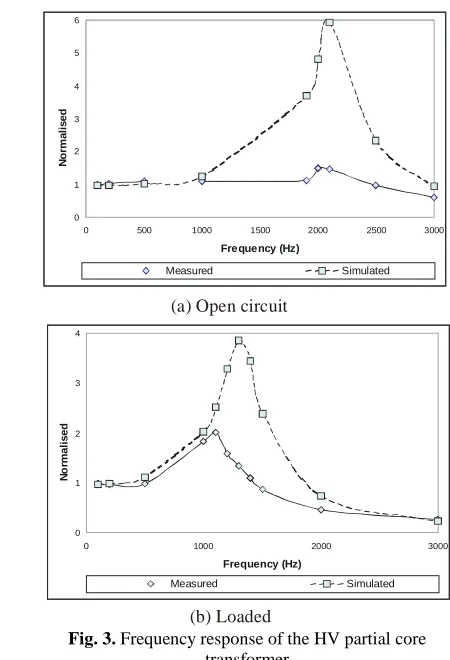
A high voltage partial core transformer with a large turns ratio was designed, built and analysed. It was designed as a scale model of a high voltage transformer for testing power system components at harmonic frequencies. Calculations of the transformer’s resonant frequencies, under both open circuit and loaded conditions, were verified by test results. This is shown in Fig. 3. The closeness of the calculated and measured results for the transformers validates the usefulness of the models derived.

5. CONCLUSIONS

A reverse design modelling technique has been applied to partial core transformers for 50Hz applications under normal operating temperature and also at liquid nitrogen temperature. It has been used for harmonic frequency analysis of partial core units. Matching results were achieved between the model calculations and test results of as-built devices. This has strengthened the use of the reverse design partial core model developed as an entry-level design tool from which more accurate designs can be made.

6. REFERENCES

[1] Bodger, P.S., Liew, M.C., and Johnstone, P.T., “A comparison of conventional and reverse transformer design”, AUPEC’2000, Brisbane, Sept 2000, pp. 80-85.

[2] Bodger, P.S., and Liew, M.C., “Reverse as-built transformer design method”, paper accepted by

IJEEE, July 2000.

[3] Enright, W.G., and Arrillaga, J, “A critique of Steinmetz model as a power transformer representation”, IJEEE, 1998, v. 35, pp. 370-375. [4] Liew, M.C., and Bodger, P.S., “Partial core

transformer design using reverse modelling techniques”, submitted to IEE Proceedings In

Electric Power Applications, Mar 2001.

0 1 2 3 4 5 6

0 500 1000 1500 2000 2500 3000

Frequency (Hz)

No

rm

a

li

s

e

d

Measured Simulated

0 1 2 3 4

0 1000 2000 3000

Frequency (Hz)

N

o

rm

a

lis

e

d

Measured Simulated

(a) Open circuit

(b) Loaded

Fig. 3. Frequency response of the HV partial core

transformer

[5] Liew, M.C., and Bodger, P.S., “Partial core transformers at harmonic frequencies”, submitted

to IEE Proceedings In Electric Power

Applications, May 2001.

[6] Say, M.G., Alternating Current Machines, Longman Scientific & Technical, England, 1983. [7] Slemon, G.R., and Straughen, A., Electric

Machines, Addison-Wesley, Inc., USA, 1980.

[8] Liew, M.C., and Bodger, P.S., “Operating partial core transformers under liquid nitrogen conditions”, paper accepted by IEE Proceedings

In Electric Power Applications, Feb 2001.

[9] Snelling, E.C., Soft Ferrite: Properties and

Applications, Butterworth & Co. Ltd, London, 2nd

edition, 1988.

[10]Liew, M.C., and Bodger, P.S., “Incorporating capacitance into partial core transformer models for Harmonic Frequency Analysis”, submitted to

IEE Proceedings In Electric Power Applications,

[image:6.595.291.516.82.412.2]