The Static Characteristic Loop and the External
Demagnetizing Factor
J. Takacs1*, Gy. Kovacs2, L. K. Varga3
1Department of Engineering Science, University of Oxford, Oxford, UK; 2Department of Materials Physics, Eötvös Loránd
Univer-sity, Budapest, Hungary; 3Research Institute for Solid State Physics and Optics, Budapest, Hungary.
Email: *[email protected]
Received June 22nd, 2012; revised July 26th, 2012; accepted August 29th, 2012
ABSTRACT
In this paper we demonstrate, that shearing is changing only one parameter of the static loop. By using the shearing factor Ns,linked to the widely used, demagnetization coefficient ND, we show the one parameter link between the static un-sheared and that of the sheared saturation loop, obtained by a non-toroidal, open circuit hysteresis measurement. The paper illustrates the simple relation between open circuit loop data and measured real static saturation data. The pro-posed theory is illustrated by using the hyperbolic model. For experimental illustration, tests results are used, which were carried out on two closed and open toroidal samples, made of NO Fe-Si electrical steel sheet, mimicking the de-magnetization effect of the open circuit VSM measurement. These are both theoretical and experimental demonstrations, that shearing only changes the inclination of the static hysteresis loop. These test results, presented here, agree very well with the calculated results, based on the proposed method.
Keywords: Magnetism; Hysteresis; Modelling; Shearing
1. Introduction
A practical way of characterising a magnetic material is to measure its static hysteresis loop in a closed magnetic circuit. This usually takes form in a toroid or an Epstein square [1], which minimises most of the stray and side effects of other measuring methods. This however is dif-ficult in practice, considering the shapes and sizes of the samples of the magnetic materials in industrial applica-tions. Since the shape of the sample changes its measured magnetic properties, it is desirable to use samples from the final product, which normally come in the shape of a rod or a sheet, for industrial purposes. This however cre-ates some difficulties, with making them into a toroid or Epstein square sample. Most test results therefore are obtained by using VSM (Vibrating-sample Magnetome-ter) [1-3] method. This method, with excellent repeat-ability, is now a widely accepted for industrial tests. The data however suffers from the effect of demagneti-zation, due to the open circuit geometry of the measuring arrangement. The need, to obtain the real, static parame-ters from measured data of the tested materials, has mo-tivated people to work out various methods to reduce the effects, influencing the measured data [4-7].
At the beginning we have assumed that, only one of
the calculated parameters is affected by the external de-magnetization. Test results showed, that this assumption was right. It is possible to work out the un-sheared pa-rameters (equivalent to closed circuit toroidal measure-ments) from the open circuit results of a VSM results. It will be shown, that this procedure requires only change in the effective slope of the loop with no change in the other major parameters of the modelled sample [8].
It was initially assumed that, the error coming from the ever present internal demagnetisation and from other sources is smaller than the [9] (usually at least an order of magnitude smaller) effect of shearing. This is however only conditionally true and all major models (like the Moving Preisach and Dinamic Jiles-Atherton etc.) [10,11] are modified to include, the ever present, internal de-magnetization. We also assumed that the effect of shear-ing depends only on the magnitude of the demagnetiza-tion factor and the mechanical treatment not introducing changes in the magnetic properties of the materials. Also assumed, that it is independent of the method of meas-urement.
Cullity, who studied the effect of shearing on the in-ternal demagnetization in detail, published the relation specifically to the shape and size of the specimen in graphical form [11-15]. In spite of all the assumptions made, the agreement between the theoretical and
perimental results is remarkable. Further experiments are in progress for further verification this simplified method. Work is also extended to include the so far neglected effects to improve on the accuracy.
2. Measuring Arrangements
Preceding the test, the toroidal sample was carefully de-magnetized by applying an alternating field of f = 10 Hz with logarithmically decreasing amplitude in 5000 steps from saturation to zero [1,2]. The hysteresis loop was measured with a triangular excitation at a frequency of
[image:2.595.344.538.263.393.2] [image:2.595.69.281.516.707.2]f = 0.001 Hz and integrated with a Walker integrator (see Figure 1). The rate of change of the field here is de-pendent on both the frequency f and field amplitude Hm therefore at Hm = 20 A/m, the rate of change, comes to dH/dt = 4f·Hm = 0.08 A/m·s.
The static hystersis loop can only be obtained at low rate of change, particularly when the extremely soft sam-ple has a characteristic square-like hysteresis loop [1,2].
To avoid phase shift between H and B, the current measuring resistance R (see Figure 1) has always satis-fied the 2πfL << R criterion.
Although the same test was repeated on ultrasoft, Fi-nemet, from nanocrystalline to Mn-Zn ferrite, NO Fe-Si and low and high carbon steel cores, due to the limited length of the paper, here only the data of one illustrative experiment are included.
3. Description of the Model
The analytical approach is based on the assumption, that in general, particularly in case of soft irons, there are three parallel processes, dominating the overall magneti-zation process i.e. the reversible and irreversible domain wall movement (DWM), the reversible and irreversible
Walker Digital oscilloscope GPIB card
N1
GPIB card
< I U
A/D
Signal gen P/S
N2 R
Figure 1. Schematic block diagram of an experimental ar-rangement for measuring the toroid sample.
domain rotation (DR) and the domain wall annihilation and nucleation (DWAN) processes.Although these proc- esses are interlinked, they can be mathematically formu-lated separately and combined, by using Maxwell’s su-perposition principle. They individually dominate the low, middle and near saturated region of magnetization and all are supposed to have sigmoid shapes. This model is already used in number of applications [15-18] and it is well documented in the literature therefore, here only a brief summary of the relevant formulation will be given in, canonic form [19,20].
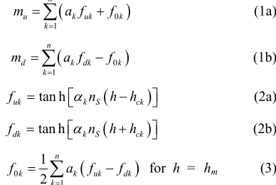
The contribution of the individual processes to the combined hysteresis loop can be described by the fol-lowing normalized mathematical equations.
01 n
u k uk k
m a f f
k
k(1a)
01 n d k dk
k
m a f f
(1b)
tan h
uk k S ck
f n hh (2a)
tan h
dk k S ck
f n hh (2b)
0 1 1 2
n
k k uk
k dk
f a f f
for h = hm (3)Here fuk and fdk are the normalized ascending and de-scending magnetization functions respectively, h is the field excitation and hckis the coercivity of the kthprocess.
ak is the amplitude of the component processes present,
αk is the slope, nS is the shearing factor (nS is unity for un-sheared loops, see later) and f0k is the integration con-stant [7,21], while hm represents the maximum field ex-citation. The index k refers to the individual component processes and n is the total number of processes involved. For most of the magnetic materials used in practice, n
equals 3 (see beginning of this section).
4. Experimental Results
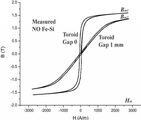
We proposed at the beginning, that the changes in the shape of the hystetesis loop measured on a closed toroid can be described by an appropriate change in the αknS product (see Equation (2)). Here αk represents the slope of the major loop, measured on a toroid sample (for nS = 1, nD = 0) in the model. For demonstration, we used the measurements on a toroidal sample made of NO Fe-Si soft magnetic material. The geometrical details of the toroids used, in the experiment, were: Dex = 25 mm, Din = 15 mm and thickness d = 0.5 mm [1].
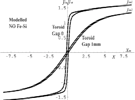
were cut in the magnetic circuit at a slow rate and the measurement was repeated. Great care was taken not to introduce additional side effects at cutting. This was for the simulation of an open-loop VSM measurement with the same ND and NS. The two hystetesis loops (before and after cutting) are shown in Figure 2. The measured loop, without the gap, was modelled by using Equations (1)-(3). When the iteration (manual or computerised) produced the best fit to the measured curve, the normalized and the equivalent physical values can be easily be read from the two coordinate systems (normalized and measured), as shown in Figure 3.
The iteration yielded the following normalised (lower case letters) and corresponding physical parameters (cap-ital letters) for the best fit:
a1 = 1.17, a2 = 0.14, a3= 0.35,
α1 = 4.5, α2 = 1.2, α3 = 0.143,
hc1 = 0.115, hc2 = 0.45, hc3 = 0.575,
hm = 7.5.
Corresponding to:
A1=1.17 T, A2 = 0.14 T, A3= 0.35 T,
Hc1 = 44 A/m, Hc2= 164.9 A/m, Hc3 = 210.75 A/m.
Hm = 2750 A/m.
The normalization: 1b = 1T, 1h = 382.6 A/m.
By altering the shearing coefficient ns, in the iteration and using the new values of α1·nS= 0.28, α2·nS = 0.073, and α3·nS = 0.0087, we obtained the closest fit to the sheared hystetesis loop. The best fit appeared to be, when
nS was around 0.061.
[image:3.595.310.538.87.255.2]From the geometry of the magnetic circuit, by using the magnetic Ohm’s law, ND (see Equation 7 for the rela-tion between ND and NS) the demagnetization factor, can be calculated by using Equations (4) and (5). We as-sumed here, that the amplitude of the magnetization vec-tor is the same in the iron as in the air gap. So:
[image:3.595.306.538.375.536.2]Figure 2. The major hysteresis loops of a NO Fe-Si sample measured on a toroid with and without 1 mm gap.
Figure 3. The measured and calculated hysteresis loops of NO Fe-Si material with and without external demagnetiza-tion.
a i
ii a i a i
i a a i a i a
H l l H
B l l l l
A
l l l l
(4)
whenμir relative permeability is used and it is assumed that la li then
0
0
1 ir
ir eff D ir
H B
N
H (5)
where
eff S
H HN (6)
is the effective magnetic field excitation. 1
1 S
D ir
N
N
(7) or in normalised form
1 1 S
D ir
n
n
(8)
Here li and la are the mean paths of iron and air respec-tively, μi and μa represent the permeability of iron and air (free space) and A is the cross section area of the iron core. It shows that, when NS the shearing coefficient is unity (no shearing), then the ND demagnetization factor is zero. The expression in (9) represents the effective per-meability.
1 ir
ieff ir S
D ir
N N
[image:3.595.58.285.514.707.2]By using the geometrical details of the toroid, given above with 1 mm effective gap, the physical shearing coefficient numerical value will come to
1
1 16.5
S
D ir
N
N
1
(10)
[image:4.595.59.286.542.710.2]here the initial permeability, calculated from the meas-ured static hysteresis loop data of the soft iron sample, was around μi = 1000.
Figure 4 depicts the calculated major loops.
In the second experiment the closed toroidal sample was magnetized into deeper saturation by applying a high
Hm = 4125 A/m maximum excitation. Following that, two 1.5 mm cut (effective 3 mm gap) were made in the toroid and the measurement was repeated.
This time however the maximum excitation was in-creased to approach Bm = 1.68 T, achieved without the gap.
The loops were modelled by using the same numerical parameters at a larger hm maximum field excitation. The resulted loops (measured and calculated) are depicted in Figure 3. The agreement between the experimental result and the modelled one is extremely close.
Other additional factors like the internal, shape de-magnetization factors and/or stresses were taken as neg-ligibly small.
The separation and calculation of αk and nS from the experimentally obtained αk·nS product, requires the pres-ence of two invariants in the transformation.
It is imperative to look at the two loops (un-sheared and sheared) at the same maximum magnetization (or as near as possible). Under this condition we can claim to have the necessary two invariants i.e. the coercivity and the maximum magnetisation.
It can be shown, that the two smaller processes (DR, DWAM) have often a negligible effect on the overall coercivity and experience shows that in most applications,
Figure 4. The modelled major loops before and after shear-ing.
particularly for soft irons, it is accurate enough in most cases to use the equations describing the dominant proc-ess. The proposal is valid, however, when the DR and DWAM processes are not negligible. All resultant pa-rameters, required for the transformation can be calcu-lated (see Appendix) from the parameters of the proc-esses involved. It is enough therefore to demonstrate the process by using one major component [22]. On this ground the present example is given entirely for illustra-tive purposes.
By using (2a), we can write for the sheared and the un-sheared dominant loop:
1tan h 1 m1 c1 1tan h 1 S m s1
a h h a n h hc1
(11)(nS being unity in the first case)
From this, the shearing coefficient nS may be calcu-lated as:
m1 1 m1 1
c S
s c
h h
n
h h
(12) where hm1 and hm1s are the amplitudes of field excitations necessary to achieve the same maximum magnetization in the un-sheared and the sheared sample respectively.
In soft steel, when the coercivity hc is small relative to the peak excitation, it is often good enough to use the ratio of the maximum field, from the saturation loop, measured by VSM. In the knowledge of nSthe value of
ακ could be calculated from the measured 1nS product. The external shearing coefficients, calculated from the measured data was ns = 0.065 for the first experiment (1 mm gap) and ns = 0.02 for the second one (3 mm gap). Some allowances should be made to the inherent internal demagnetization present in all type of measurement [2]. The estimated value of the internal demagnetization field was max 0.2 T [9].
From the second invariant, the ratio between the arc-tanh values of the remanences (sheared and un-sheared) (see Equation 2(b)) is also equal to nS.
The measured remanence of the 1 mm gap sample was 0.032 T at Bm = 1.41 T, while the corresponding mod-elled figure was 0.035 T. In the case of the 3 mm gap sample, the measured and the modelled remanence fig-ures were 0.0085 T and 0.0066 T respectively, taken at
Bm = 1.5 T. Based on these figures, Br the projected re-manence of the loop, transformed back onto the un- sheared (nS = 1 and nD = 0 ) plane came to 0.636 T.
It can be shown also, that the transformation does not change the area enclosed by the hysteresis loop, therefore sheared or un-seared, it has the same hyteretic losses.
5. Conclusion
parame-ters of the soft sample. It is also shown, that the external demagnetization affects one parameter only, namely the effective slope (i.e. nSα) of the hysteresis loop. From the sample’s geometry the shearing coefficient can often be calculated. With the proposed method and the knowledge of ND [2] one can exploit the advantage of the open ge-ometry measuring methods for unusual samples (i.e. balls, sheets or rods with known ND) and calculate the equiva-lent closed circuit static parameters.
The transformation is based on the two invariants, the coercivity and the maximum excitation.
This model independent transformation can be an use-ful tool in practice, in experimental work as well as in theoretical applications. The very close agreement be-tween the theoretical and experimental results, the rela-tive simplicity of the procedure and accuracy demon-strates the applicability of the proposed method in prac-tical cases.
REFERENCES
[1] F. Fiorillo, “Measurement and Characterisation of Mag-netic Materials,” Academic Press, Torino, 2004.
[2] D. Jiles, “Introduction to Magnetism and Magnetic Mate-rials,” Chapman and Hall, New York, 1998.
[3] S. Foner, “The Vibrating Sample Magnetometer: Experi-ences of a Volunteer (Invited),” Journal of Applied Phys-ics, Vol. 79, No. 8, 1996, p. 4740. doi:10.1063/1.361657 [4] D. B. Clarke, “Demagnetization Factors of Ringcores,”
IEEE Transactions on Magnetics, Vol. 35, No. 6, 1999,
pp. 4440-4444. doi:10.1109/20.809135
[5] Zs. Szabo and A. Ivanyi, “Demagnetizing Field in Ferro-magnetic Sheet,” Physica B: Condensed Matter, Vol. 306, No. 1-4, 2010, pp. 172-177.
doi:10.1016/S0921-4526(01)00999-1
[6] T. Nakata, N. Takahashi, K. Fujiwara, M. Nakano, Y. Ogura and K. Matshubara, “An Improved Method for Determining the DC Magnetization Curve Using a Ring Specimen,” IEEE Transactions on Magnetics, Vol. 28, No. 5, 1992, pp. 2456-2458. doi:10.1109/20.179524 [7] J. Takacs, “Mathematics of Hysteretic Phenomena,” Wi-
ley-VCH, Berlin, 2003.
[8] J. Takács, “A Phenomenological Mathematical Model of Hysteresis,” International Journal for Computation and
Mathematics in Electrical and Electronic Engineering,
Vol. 20. No. 4., 2001, pp. 1002-1005.
[9] E. Della Torre and F. Vajda, “Parameter Identification of the Complete-Moving-Hysteresis Model Using Major Loop Data,” IEEE Transactions on Magnetics, Vol. 30, No. 6, 1994, pp. 4987-5000. doi:10.1109/20.334286
[10] D. C. Jiles and J. B. Thoelke, “Theory of Ferromagnetic Hysteresis: Determination of Model Parameters from Experimental Hysteresis Loops,” IEEE Transactions on
Magnetics, Vol. 25, No. 5, 1989, pp. 3928-3930.
doi:10.1109/20.42480
[11] B. D. Cullity, “Introduction to Magnetic Materials,” Ad-dison-Wesley, Reading, 1972, p. 1014.
[12] D. X. Chen, J. A. Brug and R. B. Goldfarb, “ Demagnet-izing Factors for Cylinders,” IEEE Transactions on
Magnetics,Vol. 27, No. 4, 1991, pp. 3601-3619.
doi:10.1109/20.102932
[13] J. H. Paterson, S. J. Cooke and A. D. R. Phelps, “ Fi-nite-Difference Calculation of Demagnetizing Factors for Shapes with Cylindrical Symmetry,” Journal of
Magnet-ism and Magnetic Materials, Vol. 177-181, 1998, pp.
1472-1473. doi:10.1016/S0304-8853(97)00788-9 [14] K. Tang, H. W. Zhang, Q. Y. Wen and Z. Y. Zhong,
“Demagnetization Field of Ferromagnetic Equilateral Triangular Prisms,” Physica B: Condensed Matter, Vol. 363, No. 1-4, 2005, pp. 96-101.
doi:10.1016/j.physb.2005.03.007
[15] J. A. Osborn, “Demagnetizing Factors of the General Ellipsoid,” Physical Review, Vol. 67, No. 11-12, 1945, pp. 351-357. doi:10.1103/PhysRev.67.351
[16] L. K. Varga, Gy. Kovács and J. Takács, “Modeling the Overlapping, Simultaneous Magnetization Processes in Ultrasoft Nanocrystalline Alloys,” Journal of Magnetism
and Magnetic Materials, Vol. 320, No. 3-4, 2008, pp.
L26-L29. doi:10.1016/j.jmmm.2007.06.008
[17] J. Takacs, Gy. Kovacs and L. K. Varga,Journal of
Mag-netism and Magnetic Materials,Vol. 320, No. 20, 2008, p.
1016.
[18] J. Takacs, “Analytical Way to Model Magnetic Tran-sients and Accommodation,” Physica B: Condensed Mat-ter, Vol. 387. No. 1-2, 2007, pp. 217-221.
doi:10.1016/j.physb.2006.04.007
[19] J. Takacs and I. Meszaros, “Separation of Magnetic Phases in Alloys,” Physica B: Condensed Matter, Vol. 403, No. 18, 2008, pp. 3137-3140.
doi:10.1016/j.physb.2008.03.023
[20] J. Takacs, “The Everett Integral and Its Analytical Ap-proximation,” In: L. Malkinski, Ed., Magnetic Materials, Intech Publication, 2012.
[21] I. D. Mayergoyz, “Mathematical Models of Hysteresis
and their Applications,” Academic Press, Elsevier, New
York, 2008.
[22] J. Takacs, Gy. Kovacs and L. K. Varga, “Hysteresis Re-versal,” Physica B: Condensed Matter, Vol. 403, No. 13- 16, 2008, pp. 2293-2297.
Appendix
The single equivalent tanh function can be calculated from (14), (15), (16), and (17) as shown in (18), (19), (20) and (21).
0 0 0 0 0
1 1 1
01 2 2 2 02
tan h tan h
tan h
u u c
c c
y a h f
a h h
f a h h
f
2
(13)
where the new integration constant is:
0 01 0
f f f (14)
The remanence of the resultant hysteresis of the two process magnetization is described from (1b) and (2b) (for h = 0) as:
0 0 0 1 1
2 2
tan h tan h tan h
c c
c
a h a
a h
1
2
h
2
(15)
The maximum magnetization amplitude a0 is:
0 1
a a a (16) From (15) α0hc0 can be calculated. From the firs
de-rivative of (2b) by h comes:
2 2
0 a1 1 sech sech 1hc1 a2 2 2hc2 a0 sech 0 0
2
c
h (17)
In the knowledge a0andα0the hc0 can also be calculated.
1 1 1 2 2 2 0 0
0 1
arctnh tanh tanh
u a a h hc a h hc hc 0
(18)
and
1 1 1 2 2 2 0 0
0 1
arctnh tanh tanh
d a a h hc a h hc hc 0
(19)
From (15), (16), (17), (18) and (19) all parameters can be calculated for
0u 0tanh 0 u c0
y a h h f0
0
(20)
and
0d 0tanh 0 u c0
y a h h f (21)
as functions of the field excitation h.