The properties of the groups ON, SON, Sn and An

GROUPS ON' SON, Sn AND An

A thesis

submitted in partial fulfilment of the requirements for the Degree

of

Doctor of Philosophy in Physics in the

University of Canterbury

by

Luan Dehuai

PREFACE CHAPTER 1 2 3. PAGE 1

THE REPRESENTATIONS OF THE SYMMETRIC GROUPS 6

1.1 THE GROUP S 6

n

1.2 THE PROJECTIVE REPRESENTATIONS OF FINITE 9 GROUPS

1.3 THE ORDINARY REPRESENTATIONS OF Sn 1.4 THE SPIN REPRESENTATIONS OF Sn 1.5 PROPERTIES OF ASSOCIATED AND

SELF-ASSOCIATED REPRESENTATIONS

THE SYMMETRIC FUNCTIONS 2.1 THE BASIC FUNCTIONS

2.2 THE RELATIONS BETWEEN SYMMETRIC FUNCTIONS 2.3 SCHUR FUNCTIONS

2.4 RAISING OPERATORS

2.5 THE OUTER PRODUCT OF S-FUNCTIONS 2.6 THE SKEW S-FUNCTIONS

2.7 PARTITIONS, FRAMES AND NUMBERINGS 2.8 S-FUNCTION SERIES

2.9 HALL-LITTLEWOOD FUNCTIONS AND Q-FUNCTIONS

SYMMETRIC FUNCTIONS AND THE REPRESENTATIONS OF GROUPS

3.1 IMMANANTS OF MATRICES

4 3.2 3.3 3.4 3.5 3.6

SCHUR FUNCTIONS AND SYMMETRIC GROUPS SCHUR FUNCTIONS AND UNITARY GROUP

THE OUTER PRODUCT OR IRREPS OF SYMMETRIC GROUP

THE INNER PRODUCT OF S'!:"•FUNCTIONS Q-FUNCTIONS AND SPIN IRREPS OF SYMMETRIC GROUP

3.7 OUTER PRODUCT OF Q-FUNCTIONS

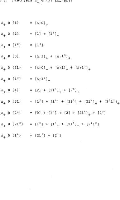
3.8 INNER PRODUCT OF Q- AND S-FUNCTIONS 3.9 THE PLETHYSM OF S-FUNCTIONS

3.10 PLETHYSMS AND BRANCHING RULES 3.11 INNER PLETHYSMS OF S-FUNCTIONS 3.12 CLASSIFICATION OF IRREPS

THE REPRESENTATIONS OF THE ORTHOGONAL AND ROTATION GROUPS

4.1

4.2 4.3 4.4 4.5

ORTHOGONAL GROUP ON AND ROTATIONS GROUPS SON

THE REPRESENTATIONS OF ON DIMENSIONS OF IRREPS OF ON BRANCHING RULES FOR ON

+

ON_₁ KRONECKER PRODUCTS OF THE IRREPS OF ON

I Kronecker products of tensor irreps 65 68 69 70 73 73 76 77 82 85 87 91 91 92 97 99 103 103

II Kronecker products of spin irreps 104 III Kronecker products of tensor and 107

5

4.6 4.7

PLETHYSM OF ON

SYMMETRIZED KRONECKER SQUARE OF IRREPS OF ON

4.8 REPRESENTATIONS OF SON 4.9 DIFFERENCE IRREPS FOR so

₂

~

4.10 KRONECKER PRODUCTS OF IRREPS OF.

so

₂

v

I Basic Kronecker products

II Kronecker products of tensor irreps 107 108 111 112 115 115 117

III Kronecker products of spin irreps 119

IV Kronecker products of tensor 124 with spin irreps

4.11 PLETHYSMS OF SON

4.12 SYMMETRIZED KRONECKER SQUARE AND THE CLASSIFICATION OF IRREPS OF SON

4.13 RESOLUTION OF THE BASIC SPIN KRONECKER CUBES OF SON

126 129

133

4.14 RESOLUTION OF THE BASIC SPIN KRONECKER 138 FOURTH POWERS OF S0

₂

~

THE REPRESENTATIONS OF SYMMETRIC GROUPS Sn - THE METHOD OF REDUCED NOTATION

5.1

5.2

AN n-INDEPENDENT REDUCED NOTATION FOR THE ORDINARY IRREPS OF S

n

THE SYMMETRIC GROUP Sn AS A SUBGROUP OF On.

143

143

6

5.3 REDUCED NOTATION FOR SPIN IRREPS OF Sn 5.4

5.5 5.6

DIMENSIONS OF IRREPS OF S IN REDUCED

n

NOTATION THE S

+

S

1 BRANCHING RULE

n

n-KRONECKER PRODUCTS IN REDUCED NOTATION I Kronecker products of ordinary

irreps 146 151 154 155 155

II Kronecker products of basic spin 157 with ordinary irreps

III Kronecker products of spin with 161 ordinary irreps

IV Kronecker products of spin irreps 166 5.7 SYMMETRIZED KRONECKER SQUARES AND THE 170

CLASSIFICATION OF IRREPS OF Sn

5.8 RESOLUTION OF THE BASIC SPIN KRONECKER 185 CUBES FOR so2\!+l

THE REPRESENTATIONS OF ALTERNATING GROUP An - THE METHOD OF REDUCED NOTATION

6.1 6.2 6.3 6.4 6.5 6.6 6.7

ALTERNATING GROUP A

n

THE IRREPS OF An sn

+

An

The A

_n

+

A

_n-

l BRANCHING RULES DIFFERENCE CHARACTERS FOR A

n

KRONECKER PRODUCTS OF THE IRREPS OF An SYMMETRIZED KRONECKER SQUARES AND THE CLASSIFICATION OF IRREPS OF A

n

REFERENCES

APPENDIX: Publications

TABLE I II III IV

v

VI VII VIII IX X XI XII

The table of Bm[qJ

Table of spin character for a-regular

classes of Sa

Dimensions of tensor and spin irreps of 01o

Plethysms o" ® {~} for S01o

Plethysms ~+ ® {~} for S01o Branching rules On

+

Sn

[~;0)

+

<O>'t

I

<TI>

Reduced Dimensions for Sn spin irreps

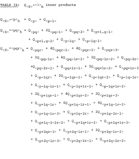
Q<O> o <~>n inner products

Expansion of spin irreps in terms of the

basic spin irreps and ordinary irreps of Sn

Symmetrized Kronecker squares for the

ordinary irreps of sn

Table of spin character for a-regular

classes Ae

PREFACE

The problems of group theory applied in physics often are reduced to the calculation of the dimensions, the

branching rules, the resolution of the Kronecker products, the symmetrized powers and the classification of the

irredicuble representations (irreps) for a wide variety of groups. The orthogonal ON and its subgroups, especially

the rotation groups SON' symmetric groups Sn and the alternating groups A have been of special interest to physicists.

n

The n-dimensional rotation groups play an important role in many areas of physics and chemistry. They arise, for example, in the description of symmetrized orbitals in quantum chemistry (Wybourne 1973), in fermion many body theory (Fukutome et al 1977), in boson models of nuclei

(Arima and Iachello 1976), grand unified theories (Gell-Mann et al 1978) and in supergravity theories (Cremmer and Julia 19 7 8) •

Interest in the rotation groups has greatly increased in recent times with study of candidate groups for grand unified theories of the weak, electromagnetic and strong interactions. The group S010 appears to be of particular significance (Fritzschand Minkowski 1975, Chanowitz et al 1979, Buras et al 1978, Georgi and Nanopoulos, 1979, Witten 19 79) .

The symmetric group has long been of interest to physicists and chemists who have sought to exploit the permutational

For An in physics the isomorphisms C3 ~As, T ~ A4 and I ~ As are well-known in solid state and molecular physics (Lax 1974).

The subject of my thesis is devoted to problems

concerning dimensions, branching rules and the resolution of the Kronecker products etc for the groups ON' SON, Sn and A .

n

This thesis is organized as follows: In chapter 1 a brief statement is given about the results of the theory of representations of group S both in ordinary and spin

n

representations that will later be used. On spin represen-tations, I prefer the concept of projective representations to that of the ordinary representation of double groups. Given a brief statement about projective representation I restate the familiar results gotten from double groups from the standpoint of projective representations. In the end of this chapter I present some results relevant to associated and self-associated representations.

Chapter 3 is devoted to the relation between the symmetric functions and the representations of groups. The relationship between S-functions, Q-functions and the representation theory of groups is outlined. I present the definitions of the inner product of S-functions and Q-functions which play an important role for resolving the Kronecker product of the spin and ordinary irreps of Sn and point out the relation between branching rules, skew S-functions and Q-functions.

The results given in chapter 4 are explicit formulae for a complete set of fundamental products from which all possible products of irreps of ON and SON may be evaluated both for n

=

2v and for n

=

2v + 1. The explicit resolution of the basic Kronecker squares into their symmetric and

antisymmetric parts is then given, followed by a complete resolution of the Kronecker cubes of the basic spin irreps of

so

₂v+l and

so

₂v, together with a prescription for analysing explicitly the Kronecker fourth powers of these irreps.

These results permit analysis of the Kronecker second, third and fourth powers of any irreps (spin or tensor) of the

groups

so

₂v+l and

so

₂v to be made unambiguously. These results are given in a general form that is essentially independent of N, the dimension of SON.

many of the results have been given in an n-independent form using a "reduced notation" for labelling the irreducible

representations of Sn. But the spin (or projective) irreps of Sn have received far less attention. As long ago as 1911,

Issia Schur, having previously investigated the representations of any finite group by linear fractional (Schur 1904, 1907) directed his attention to the study of spin representation of Sn (Schur 1911) . Methods of constructing spin characters tables of Sn are of recent origin (Morris 1962a, Read 1977) . Remarkably little is known about the resolution of Kronecker products involving the spin representations apart from the explicit use of character tables. This contrasts strongly

with the corresponding reduction of the ordinary representation of Sn. In chapter 5 I give attention to the problems mentioned above. I establish an On ~ Sn embedding and the formation

of branching rules for On

+

Sn is then considered, leading to a reduced notation for the spin representations of Sn' making possible many n-independent results. The first

application is to discuss the n-independence of the dimensions of the spin representations of Sn. In order to facilitate the reduced notation, a special Young raising operator R

0 j

is introduced. These results, together with consideration

of diffec~nce characters of Sn' give a general procedure for

resolving arbitrary Kronecker products without the explicit use of character tables. We are then able to use the method of plethysm to resolve Kronecker squares of the spin

orthogonal, symplectic or complex characters.

In the last chapter, chapter 6, I extend the reduced notation developed in cha p ter 5 to An, the subgroup of Sn, leading to an essentially n-independent treatment of the properties of the representations of An. Branching rules for Sn

+

An are developed. The difference character for the irreducible representation of An are established and used to establish a series of algorithms for evaluating Kronecker products and plethysms of spin and ordinary irreps of An. In the concluding section the systematic classification of the irreps of An is given.

I would like to express my gratitude to my supervisor,

Professor B.G. Wybourne, for his continued support and guidance, particularly for demonstrating the power of symmetric functions and difference characters to me. Also I would like to express thanks to Dr P.H. Butler for numerous discussions. Appreciation is also recorded of Dr R.C. King in preparing the manuscript of the material included in chapter 4 for publication.

Lastly, I would like to thank my wi , Wang Shuxian, for looking my family and children when I am on leave and Janet Warburton for her excellent job of typing a very

difficult manuscript.

Christchu~ch

New Zealand February 1982

CHAPTER 1

THE REPRESENTATIONS OF THE SYMMETRIC GROUPS

1.1 THE GROUP Sn

The n! permutations of n objects form a group called the symmetric group sn.

Any permutation can be resolved into the product of cycles. If V1

=

no.of one-cycles, Vz =no. of two-cycles,

etc., then since there are just n symbols for a given permutation in sn

v

The cycle structure may be designated as (lv1 _2v2

• • • n n)

or just (v) . All permutations in Sn which have the same cycle structure (v) form a conjugate class in Sn. Thus each solution of (1.1) for positive integers V1 1V 2 , •••,vn

gives a class in Sn; hence the number of classes is just the number of such solutions. Let

V1 + Vz +

Vz + ••• + vn

=

A2

(1.1)

then

(1.3a) and

(1.3b)

Thus each solution of (1.1) corresponds to an ordered

partition of n and wA is called the weight of partition (A). Ordinarily a partition (;\)

=

(Al, Az, ••• ApA' 0,0,0) of n is writ ten (A) = (A 1 , A 2 , • • • _{APA) i.e. we omit the} Ai that are zero. Also, if several of the Ai are equal

we use exponents to shorten the notation. Thus the partitions (4000), (3100), (2200), (2110) and (1111) of 4 are usually written in the abbreviated forms

The number of classes in sn is equal to the number of partitions into positive integers such that (1.3) is

satisfied.

Given a partition as in (1.3) there is a corresponding cycle structure, namely

Cycle structures involving an even number of even length cycles correspond to even permutations and are called even classes while all other cycle structures are odd and are referred to as odd classes.

For later convenience we shall adopt the convention of listing the cycle structures in order of their decreasing length and omit all cycles with exponents

v.

=

0. Thus in 84,

l

we designate the classes as (1 4),(212) , (.22),(31) and (4) with

the (1 4), (22_{) and (31) classes involving even permutations} only.

The number of distinct permutations of 8n having the

v

1 t t ( n 2v2 1v1) .

eye e s rue ure n . . . 1s

g ( v)

Thus for 8 4 , we have

partition cycle structure no. of element in class

( 4) ( 14) 1

( 31) ( 212 ) 6

( 2 2) ( 2 2) ₃

( 212 ) ( 31) 8

( 14) ( 4) 6

We note that the total number of elements is equal to 4! which is the order of 84.

1.2 THE PROJECTIVE REPRESENTATIONS OF FINITE GROUPS We now consider a few of the relevant properties of irreducible projective representations (i.p.r) of finite

groups (Schur 1911, Curtis and Reiner, 1962 and Dornhoff, 1971). Let G be a finite group, k a field and kx the multiplicative group of k, V a finite dimensional k-vector space. A projective representation of G on V is a mapping T: G + GL(V) such that

for all x,y E G

T(x) T(y)

=

a(x,y)T(xy)

T(e)

=

I (1.6)

where a(x,y) E kx. The function a:G x G + kx is called a factor set of T and T an i.p.r. if V has no proper subspace invariant under T(x), x E G. Furthermore

a(x,y)a(xy,z)

=

a(x,yz)a(y,z) x,y,z E G

a(e,e)

=

1 x E G (1.7)

If a

=

1 then T is an ordinary representation. Two factor sets a and (3 of G are termed equivalent if there is a function

X

y:G + k such that for all x,y,

a(x,y)

=

(3(x,y)y(x)y(y)y-1_(x,y)

The set H2 (G,kx) of all equivalence classes under (1.8) with multiplication {a}{S}

=

{aS} well defined forms an

)

Abelian group of equivalence classes of the factor sets

and is known as the Schur multiplier of G over k. For

Sn we have (Davies and Morris, 1974).

(n ~ 4) (1.9)

if r

=

1 the T of Sn will be called an ordinary irrep. While

if r

=

-1 Twill be called an projective or spin irrep of sn.

The centralizer C(x) of an element x E G is the

collection of elements s E G such that s x s-1 _{= x. If a}

is factor set of G, an element x E G will be termed an

a-regular element if

c:dx,s) = a(s,x) (1.10)

for all s in the centralizer of x in G. If x is a-regular

then every element which is conjugate to x in G is a-regular

and hence we may speak of an a-regular class.

Two major differences between projective and ordinary

irreps must be noted. The first one concerns the character

T T

x •

For ordinary irreps, as is well known,

x

are the class

functions, whereas in projective irreps we have (Altmann,

1979)

T 1 ( -1)-1 -1 -1 ( -~ T )

X ( gg i g- } = a g , gig a ( g i ' g ) a g, g ) X ( g i

(1.11)

The sufficient condition for the character to be a

Vg E G (1.12)

obtains for all regular elements gi E G. This class function vanishes over all the irregular elements of G.

The second difference is that the number of inequivalent irreps that can be constructed for a given factor system is not, as for ordinary irreps, equal to the number of classes. The number of distinct inequivalent i.p.r. of G with the factor set a is equal to the number of a-regular classes of G and

I

ni_

=

g i

where n. are the dimensions of the inequivalent i.p.r's 1

and g is the order of G.

(1.13)

For Sn the a-regular classes fall into two categories: (1) even permutation-classes containing only cycles of odd order; (2) odd permutation classes containing cycles of unequal orders. Thus for 87 we have the eight a-regular classes

even

(61), (52)' (43) odd

while for Ss we have nine a-regular classes

even

1.3 THE ORDINARY REPRESENTATIONS OF Sn

It is well known that for a finite group G the number of nonequivalent irreps of G is equal to the number of conjugate classes in G. For Sn' as mentioned in sec. 1.1, the number of conjugate classes is equal to the number of partitions of n, so we can use the partition (A) to label the irreps of Sn designated by [A].

Every partition (A) of n may be given a unique graphical representation in terms of n cells or nodes arranged in

PA left-adjusted rows with the i-th row containing Ai cells. These graphs are known as Young diagrams.

For n = 5 we have the diagrams

(5) (41)

IJ

II

(32)

For a given diagram (A) we can obtain another diagram from (A) by interchanging rows and columns called the

"' '

---.J

(32) (32)

If (X)

=

(A) then partition is said to be self-associated.

For example the partition (312) of 5 is self associated.

If ( A)

= (

A 1 , A 2 , • • • , Ap ) then

A

(1.14)

hence

~

(54213)

=

(63221)

I t is well known from number theory (Hardy and Wright,

1954) that the number of partitions of n into odd and

unequal parts is equal to the number of its self-associated

partitions. Every self-associated partition (A)

=

(Al 1A2 , • • •

can be related to a unique partition of odd and unequal parts

(p)

=

(pl,

P2 ...

,pk) where

p.

=

2A. - 2i + 1

l l ( 1.15)

we say (p) belongs to the self-associated partition (A).

The number of self-associated partitions for given n is

readily seen to be

(1.16)

;d

/

m parts, the summation is over m = 2, 4, ... for n even and m

=

1,3, ••• for n odd and Bm(O) are always defined as 1. Table 1 gives the value of Bm[q] (m

=

10, q ~ 10, q ~ 30).

For example for n

=

31 the number of self-associated is

B1 [15]

+

Bs [11]

+

Bs [2]

I

=

1

+

16

+

2

=

19

and for n

=

36 is

B2 [16]

+

B4 [10]

+

Bs [0]

= 9

+

23

₊

1 = 33

Another method of describing partitions, known as the Frobenious notations, will occasionally be used. The diagonal cells in a Young diagram beginning at the top left hand

corner is called the leading diagonal. The number of cells on the leading diagonal is termed the rank of the partition. If r is the rank of the partition and there are ai cells to right the leading diagonal in the ith row and hi cells below the leading diagonal in the ith column then partitions may be designated after Frobenius as

[a'

a2

... ar

l

(A)

₌

.b 1 b2 •.• br

(1.17a)

with

(A'>

[b

l b2

br]

=

al bz _ar

[image:21.595.78.531.71.397.2]

TABLE 1: The value of Bm[q]

~

1 2 3 4 5 6 7 8 9 10

0 1 1 1 1 1 1 1 1 1 1

1 1 1 1 1 1 1 1 1 1 1

2 1 2 2 2 2 2 2 2 2 2

3 1 2 3 3 3 31 3 3 3 3

4 1 3 4 5 5

I

51 5 5 5 5

5 1 3 5 6 7 7 7 7 7 7

6 1 4 7 9 10 11 11 11 11 11

7 1 4 8 11 13 14 15 15 15 15

8 1 5 10 15 18 20 21 22 22 22

9 1 5 12 18 23 26 28 29 30 30

10 1 6 14 23 30 35 38 40 41 42

11 1 6 16 27 37 44 49 52 54 55

12 1 7 19 34 47 58 65 70 73 75

13 1 7 21 39 57 71 82 89 94 97

14 1 8 24 47 70 90 105 116 123 128

15 1 8 27 54 84 110 131 146 157 164

16 1 9 30 64 101 136 164 186 201 212

17 1 9 33 72 119 163 201 230 252 267

18 1 10 37 84 141 199 248 288 318 340

19 1 10 40 94 164 235 300 352 393 423

20 1 11 44 108 192 282 364 434 488 530

21 1 11 48 120 221 331 436 525 598 653

22 1 12 52 136 255 391 522 638 732 807

23 1 12 56 150' 291 454 618 764 887 984

24 1 13 61 169 333 532 733 919 1076 1204

25 1 13 65 185 377 612 860 1090 1291 1455

26 1 14 70 206 427 709 1009 1297 1549 1761

27 1 14 75 225 480 811 1175 1527 1845 2112

28 1 15 80 249 540 931 1367 1801 2194 2534

29 1 15 85 270 603 1057 1579 2104 2592 3015

[image:22.595.92.503.119.755.2]

This may be illustrated by the partition (62432) which has the Young diagram

0

0

0

and hence the partition is of rank 3 and in the Frobenius notation is designated as

4

3

~]

Note that the numbers in each row strictly decrease, and that zeros, even two zeros one above the other, are significant. The two examples, of the Frobenius notation given below

4

3

and

represent different partitions.

Another concept called the hook plays an important part in the theory of irreps of sn. In Young diagram (A)

the square located in i-row and j-column is called

(i,j)-nodes along with the Ai-j nodes to the right of i t (called the arm of the hook) and the Aj nodes below i t (called the leg of the hook) . The length of the (i,j)-hook . h (A) I

~s .. = A. + A. + 1 - i

-

j . If we replace the

(i,j)-~J ~ _J

node of (A) by the number h ~ ~)

~J for each node, we obtain

the hook graph.

For example, the (2,2)-hook of the Young diagram

and the hook graph is

7 5 4

lj

5 3 2

4 2 1 1

'----The formula, due to Frame, Robinson and Thrall (Frame et al. 1954), for the dimension of irrep [A] of Sn in terms of the hook graph is of fascinating simplicity. The dimension of irrep [A] is

f [ A J = n ! /H ( A ) (1.20)

where H (A)

=

II

ij

h~~)

called the product of the hook lengths.

~J

From the above discussion we know that Sn has two nonequivalent one dimensional irreps [n] and [ln].

[n] corresponds to the identity irrep and [ln] to the alternating irrep. We also have the fact that [ln]· [A] is an irrep and i t will be said to be the associated irrep of [A]. It is easy to prove i t ' s Young diagram is (X) so we use [X] to label [ln] ·[A].

If [X] = [A] the [A] will be called self-associated and denoted by [A]t.

If

rXJ

~ [A], we note that [A] +

rXJ

corresponds to a reducible self-associated rep of Sn. As a consequence we shall often use [A]t with the understanding that if

[A] ~ [A] then

result

(1.21)

Here we would like to quote a/due to Littlewood (1950) (cf. Rutherford, 1948) which will be used in the following chapter.

Theorem.

[1T]

The character X(p) is given by

(1.22)

where there is one term di for each way in which the shape

.•• ,and lastly a regular application of ph spaces, and t.

where di

=

(-1) 1, ti being the sum of the numbers of

vertical steps in the h applications.

1.4 THE SPIN REPRESENTATIONS OF Sn

In Sec. 1.2 we pointed out that the H2 (Sn' Cx)

=

C2

=

{r}. Correspondingly r

=

-1, the i.r.p. of Sn also called

the spin irreps. The spin irreps of Sn may be uniquely

labelled by the ordered partitions of ti into unequal parts (Schur 1911) i.e.

with

To distinguish spin irreps from ordinary irreps of S we

n

(1.23a)

( 1. 23b)

shall use a prime. Thus [531] 1 _{is a spin irrep while [531] is}

an ordinary irrep of S9 •

The Kronecker product of ordinary irreps with spin

irreps are also spin reps (Altmann et al., 1979), so [ln] [A] 1

is a spin irrep of Sn' whose dimension is the same as the

[A] 1

, denoted by [r] 1 • If [r] 1 ~[A] 1 i t be also called

. [ t . "' _L

self-assoclated denoted by A] 1 _{and 1f [A]} 1 _{r [A]} 1 _then

[r] 1 _{will be called the associated irrep of [A]} 1 •

In fact if (n-k) is even the irrep is self-associated

while if (n-k) is odd we obtain an associated pair of spin

self-associated rep for {n-k) odd. As a consequence we shall often use [A]

,t

without regard to the parity of

(n-k) with the understanding that if (n-k) is odd then

r

A

₁

I t

=

[A

₁

I

+

[r

_{1 •}

(n-k)odd

The dimension formula for spin irreps of Sn was given long ago (Schur 1911) for a k parts partition (Al,A2, •••

where [ (n-k) /2] denotes the greatest integer.

For each value of n there is a basic spin irrep [n]

,t

of dimension 2[n/2] where [x] denotes the greatest integer less than equal to

x.

(1.24)

(1.25)

For the spin irreps of Sn' (1.12) is satisfied, so the characters are the class functions and vanish on a-irregular class. We only consider the value of characters on a-regular classes. First, considering odd a-regular classes

character of irrep [AIA2 • • • A ] I

k

is non-zero given by

[A] I

X (A)

=

i ( n-k- 1 )

I

1

A 1 A 2

. .

.

Ak/2)~

( 1. 26a) and

[A] I

X (A)

=

[A] I

while its value on every other odd a-regular classes are zero.

In dealing with the associated spin irrep when (n-k} is odd i t is useful to exploit the properties of difference characters

[A] Ill [A] I [';\]I

X = X - X (n-k} odd

Noting (1.24) we have

X [A] '

=

[A] It

<x

+ X [A ] '" ) /2 and

X

(A'] '

=

<x

[A] It - X [A ] "' ) /2

For the odd a-regular class (A1A2 ••• Ak) we have the difference character

=

i(n-k+l)/2~ArAz ••• A ) ~ k

The difference character for all other classes is zero. For even a-regular classes, Morris has established the results for n 13 as follows (Morris, 1962a) .

Let

as a3 a1

(TI) = (••• 5 3 1 )

and

(1.27)

(1.28a)

(1.28b)

then we have

(1) k

=

2

[n-2,2] 1

=

2 (p-2-t)/2 (C'tl-1) (al-4)

x(rr) 21

(2) k

=

3

[n-4, 31] 1

x(rr)

[n-5,41] 1

X ( rr)

[n-6,51] 1

X ( rr)

--=

[n-6,42] 1

X ( 1T)

=

2 (p-3-t)/2{5al (a1-l) (al-3) (al-5) (a1-8) (a 1 -10)

6!

[n-7, 43] 1

X ( 1T)

(3) k

=

4

[n-6, 321] 1

X ( 1T)

[n-7, 421] 1

X ( 1T)

=

2 (p-3-t) /2{5al (a1-l) (a1-2) (al-5) (a1-6) (a1-lO) (a1-ll) 7!

2a1a3 (a1-2) (al-5) (al-7) 4!

where in each case t

=

0 if n is even, t

=

1 if n is odd. As an example, we give the table of spin character for the a-regular classes of 88 in table II.

The Kronecker product of a spin irrep with a spin irrep is an ordinary rep as well the Kronecker product of a spin irrep with an ordinary irrep is a spin rep

(Altmann et al., 1979), so the basic spin irrep is such an irrep from which every irrep of S arise in a Kronecker

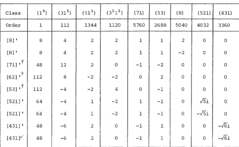
TABLE II: Table of spin character for a-regular classes of

Sa

Class ( 1 8) _{( 31} 5) (51 3) (3212) ( 71) (53) ( 8) (521) Order 1 112 1344 1120 5760 2688 5040 4032

[8] I 8 4 2 2 1 1 2 0

[8] I 8 4 2 2 1 1 -2 0

[71] I t _{48 12 2 0 -1 -2 0 0}

[62] I t _{112 8 -2 -2 0 2 0 0}

[53] I t _{112 -4 -2 4 0 -1 0 0}

[521] I 64 -4 1 -2 1 -1 0

lSi

[521] I 64 -4 1 -2 1 -1 0

-lSi

[431] I 48 -6 2 0 -1 1 0 0

[431]11 _{48 -6 2 0 -1 1}

I

0 0

(431)

3360

0

0

0

0

0

0

0

-/6i

[image:31.598.63.538.164.455.2]

1.5 PROPERTIES OF ASSOCIATED AND SELF-ASSOCIATED REPRESENTATIONS

In the previous sections we have noted that both the ordinary and spin irreps of Sn may be divided into two classes: associated and self-associated irreps. This is a general property of groups that contain the one-dimensional alternating irrep.

Two theorems concerning associated and self-associated irreps play an important role in our subsequent analysis of the properties of the irreps of Sn both in ordinary and spin cases. These theorems reinforce the usefulness of the

notation developed in the previous sections.

Theorem 1

t ""

If a group

G

contains a subgroup

H

with

A., A., A.

and

~ ~ ~

t p. ,

~

rv

p. being their respective se

~

associated pair irreps then under G

+

H

then (i)

( ii}

"' j t j"' A .

+

a .p .

+

b.; p.

~ I J ..._

associated and

where the coefficients

a~

and

b~

are non-negative integer

~ ~

multiplicity numbers.

(1.30)

Proof

(i) Suppose

1

t.

j

t

j j.v

A

+

a.p.

+

b.p.

+

c.p.

~ 1 ] ~J ~J

For A: is self-associated,

A~IH

as the subset of A: is also

~ ~ ~

self-associated hence

Al!H = _rt1H i.e.

. t _{jrv j} . t _jrv

j

J

₊

₊

J

₊

₊

a.p. b.p. c.p. = a.p. b.p. c.p.

~ J ~ J ~ J ~ J ~ J ~ J

Compare the coefficients of the two sides of the equation we have

b~

=

c~ ;

~ ~

so

A:

₊

a.p. j t + b?(p. ₊

p.)

~ 1 J ~ J J

(ii) the proof is trivial.

Theorem 2

Let A:, A., r. be self-associated and associated pair

~ ~ ~

irreps of G. The Kronecker products of the irreps of G necessarily satisfy the identities

(i) 1

t.

1

1\ X /\•

~ J

\ t.

,....,

= A X A~

~ J

k t k rv

= a .. Ak

+

b . . { Ak + Ak)

(ii) A: X

A~

=

a .. Ak k t

+

b .. (Ak k

₊

_'>:'k) (1.33)

~ _J ~J ~J

(iii) "' A. x

r.

₌

_A· X _A· (1.34)

~ _J ~ _J

(iv) if

A.

X A·

=

_aijAk k

t

+

b. ·Ak k

~ _J ~J

then

,...,

r.

A· k

t

k "' {1.35)

A. X

A·

=

X

=

a .. Ak

+

_{b. ·Ak}

~ _J ~ _{J ~J} ~J

The proof of this theorem is ~s similar as the

CHAPTER 2

THE SYMMETRIC FUNCTIONS

2.1 THE BASIC SYMMETRIC FUNCTIONS

The theory of symmetric functions play an important role in our later discussions. Here we give some facts about the theory of symmetric functions (Littlewood, 1958, Wybourne 1970).

Consider a set of countably many variables (finite or infinite)

(2.1)

Any product of powers of (x) such that

(2.2)

will be termed a monomial function.

From monomials of (2.2) we can define some basic symmetric functions.

Ix~

=

xt + X~ + X~

1

Ix~x.

=

xtx2 + XlX3 2 + X2Xl 2 + X2X3 2 + xaxr 2 + XaX2 2

1 J etc.

where the summation sign indicates that all distinct monomials in the xi's, with the exponents in a prescribed order, are to be included.

It is apparent from the above simple examples that we can define a monomial symmetric function k(A) for each partition

(A)

=

(Al,A2, ••• ,A.p) of n such that

=

k (A) ( x)

=

where the summation is over all monomials obtained from A

x P by a permutation of the variables (x) e.g.

p

particular choices of the partition (A) lead to special cases of symmetric functions.

Now consider some cases

then

is called an elementary symmetric function. Clearly

( 2. 3)

ar(r ~ 0) is the sum of all products of n distinct variables xi. For r = 0,

av

=

1 while if r > 0

(2.5)

and we define

( 2. 6)

for (A) = (A1,A2 , • • • , Ap). In three variables we have

while

The elementary symmetric functions a (x) are associated

,-with the generating function

00

I

tr 00

A(t) a _{= .ITO} (1

₊

x.t)

r=O r l= l

( 2 • 7)

(ii) if (A) = (r) then

is called the power sum symmetric function which clearly is sum of the n-th powers of x. 's i.e.

1

and we define

for (A)

=

{)q >1.2. • • • A.P) . For example, we have

while

The power sum symmetric functions are associated with the generating function

00 00 00

s (t) =

I

s t r-1 =

I

I

x.t r r-1 r=l r i=l r=l 1

00 x.

I

1

=

i=l 1-x.t

1

I

d lg 1

=

i=l dt 1-x.t

1

( 2 • 9)

(2.10)

(iii) The sum of all monomial symmetric functions of

degree r in the xi's is called the complete symmetric function or homogeneous product sum denoted by hr i.e.

h _r

=

where A ~ r denotes all the partitions of (A) of r and define

h (A)

=

h _{A 1} hAz

.

.

.

hA p for {A)

₌

{AlA2

...

Ap) . Thus

ho

=

1

hl

=

Ix1

hz

=

LXI

+

Ix1x2

hs == _Ixr

₊

_Ixtxz

₊

_Ix1xzxs

etc. and

The complete symmetric functions hr(x) are associated with the generating function

co

H(t}

=

I

r=O

co

II {1-xi t } -1

i=O

(2.12)

(2.13)

2.2 THE RELATIONS BETWEEN SYMMETRIC FUNCTIONS

The a and h may be simply related by noting that their

r r

generating functions lead to the identity

H(t)A(t)

=

1 ( 2 .15)

and hence

n

I

(-l)ra h

=

0

r=O r n-r (n=l,2,3, .•. ) (2.16)

leading to the determinantal forms

hl 1 hz hl 1

ha hz hl 1 a =

r (2.17)

. .

.

.

.

. .

.

.

.

.

. . .

• • • • • • • • • • • • • • • • • £ 1

hr h r-1 • • • • • • • • • • e • • hl and

a1 1 az a1 1 a3 az a1 1

hr = (2.18)

.

.

.

.

.

.

. .

. . .

.

.

.

. .

. . .

. .

. .

. .

. .

.

.

. .

.

.

.

1 a _r a _r-1

.

.

. . .

.

. . .

.

a1

In a similar way we find

n

I

r=l s h

r n-r (n=l,2,3, .. ) ( 2 .19)

2h2 hl

and

(-l)r-1

r'h _{. r}

=

3hs

ss

Likewise we also have

and

r!a

=

r

ra

r

h r-1

s r-1

a r-1

s r-1

2

1

1

-2

-3 (2.21)

-r+l s 1

1

1

(2.22)

1

3

(2.23)

2.3 SCHUR FUNCTIONS

There are several equivalent definitions about Schur functions or S-functions. The traditional definition is in terms of determinantal expansions involving the variables

( x) • Let (A) ~ (A1A2 • • • A) ~sa partition of r then inn

p ' .

variable (x) of the S-function {A} is defined by (Littlewood, 1950)

( \. ( !

{A} (2.24)

XI X~ X~

{21}

=

XI X~ X~

1 1 1 1 1 1

=

xi (x~-x~) + x~ (x~-xi) + x~ (xi-x~)

XI(X2-X3) + X~(X3-XI) + X~(Xl-X2)

Equation (2.24) is cumbersome in practice. However, the S-function {A} are symmetric functions and hence may be related to the symmetric functions a(A), h(A) and S(A). In fact, there exists the remarkable Jacobi-Trudi identity

(Littlewood 1958)

which in (2.24) gives

{:\} =

jh:\.-i+j!

l

with h _r

=

0 if r < 0.

From (2.26) we can define the dimension of {:\},f:\

f (A)

=

w,. - - - - -1 1

1\_ (:\.-i+j)!

l

This is the dimension of irrep [:\] of SN (James, 1978). Thus

and

{21}

=

=

h1h2 - hs

1 hl

But

and

hence we have again

If (r)

=

(~) then (Littlewood, 1950)

{:\}

_I

_{a . .}

I

~.-l+J

l

with ar

=

0 if r < 0.

(2.26)

(2.27)

(2.28)

Thus

{lr}

₌

_{ar (2.30)}

and

a2 a3

{21}

₌

₌

a1a2-as 1 a1

=

Ix1 <l.x1x2)

-

Ix1X2Xs

=

LXIX2 + 2Ix1x2xs

I t has been assumed in the definition of the S-function {A} that the parts Ai of (A) are in standard descending order and non-negative. It is convenient to be able to define the S-function {A} even when the parts are not in standard order or may be negative. In these cases consideration of the

determinantal expression (2.26) leads to a set of three rules for transforming a non-standard S-function into standard

form (Littlewood,l950). The rules are

2 •

3.

=

A. +1 then {A}

1.

If A _p < 0 then {A}

=

0 0

which are called modification rules of S-function. For example

{2332}

= -

{2242}

=

{1342}

=

0

(2.3la)

{ 2. 3lb)

(Using (2.3la} and (2.3lb) and

{2 5 -2 3} = - {2 5 4 -3}

=

0

(using (2.3la) and (2.3lc}.

2.4 RAISING OPERATORS

In the previous section we gave the relationships between {A} and other symmetric functions such as in (2.26} and

(2.29). Here we give a raising operator method to express {A} by h{A) or vice versa. (Thomas 1976}.

The Raising Operator R., (i < j} is an operator which

~J

operates on a partition (A} by increasing A. by one and

~

decreasing A. by one so that

J

• • • I A.+l,A.-1 .•. }

~ J

Consideration of (2.32) and (2.26) leads to the remarkable results

{A} =

rr

R .. ) hA i<j ~J and

hA =

rr

1 {A} i<j 1-R ..

~J

=

rr

(l+R .. + R~. +

...

) {A} i<j ~J ~J

( 2. 32)

(2.33}

(1+R13+R1 ~+ ••• ) ({321} + {330})

=

{321} + {330}

+

{420}

and then

(1+R12+Rd+ ••• } ( {321} + {330} + {42})

=

{321} + {411} + {501} + {6-11} + {33} + {42} + {51}

+ {6} + {42} + {51} + {6}

But {501}

=

0 and {6-11}

= -

{6} and hence

h32l

=

{6} + 2{51} + 2{42} + {41 2 } + {3 2} + {321}.

2.5 THE OUTER PRODUCT OF 8-FUNCTION8

The outer product of two 8-functions {~} and {v} may be defined by writing

{~v} (x)

=

{~} (x) • {v} (x) ( 2 • 35)

which may be represented as a determinant in the symmetric functions hr. Putting

r

=

p

+

P

~ v ( 2 • 36)

we have

{~·v}

=

lh

_~. + ·

·I

v

+1 .-l+J

1 r -J

(2.37)

f (J-l v)

(wl-l+w)! 1 (2.38}

=

(J-l.+V +l .-i+j)! _{~ r -J}

It is equal to

f (J..l\1) ₌ (wl-l+w)! f(J-l) f ( v) _{( 2. 39)}

w !w !

1-l \)

For example

hz ha hs hs ha

1 hl hs hlf hs

{21· 2li = 0 0 hl hz hlf

0 0 1 hl hs

0 0 0 1 hz

a result that could also be obtained by use of (2.26) by

multiplication of the determinantal expansions of {21} and

{212

} and

210

The product so defined is a symmetric function and may

be expressed as the sum of S-functions using (2.34} to give

The coefficients g A are positive integers and may be J-l\1

evaluated by the well-known Littlewood-Richardson rule

(Littlewood (1958), but we will give another procedure

due to Wybourne in section 2.7.

Hence if (A)

=

(321) then (2.32) leads to

=

(l-R12) (l-R13) (ha21-haso)

which is readily seen to be equivalent to the expansion of the determinant

ha h4 hs hl h2 h3 0 1 hl

obtained from (2.26).

Likewise use of (2.33) leads to

) (l+R1 a+R1 ~ + ••. )

(l+R2s+R2~+ ••. ){321}

But

(l+R2 ₃+R2~+ ... ) {321}

=

{321} + {330}

Equation (2.40) can be checked by the dimensional relations

2. 6 THE SKEW S-FUNC'riONS

Let (A) is the partition of wA and (~) the partition of w~ (wA > w~). wA

=

w~ possible if (A) - (~) to give

(A/~)= (0). A skewS-function, 0./~}, may be defined

(2.41)

analogously to that of {A} by the generalization of Jacobi-Trudy identity

and

{A/~}

=

lh

_{A.-~ .-i+j}

I

]. J

{'t/i1}

=

I

a

A.-~.

]. J

The dimension of {A/~} is defined by

The skew S-functions {A/~} are symmetric functions and hence may be expressed in terms of S-functions {v} of weight wA-w~. The procedure for obtaining the terms {v}

for a given {A/~} is given by expanding the determinant in (2.92) and expressing the product of hr as S-functions using (2.34) and may be written as

(2.42)

(2.43)

(2.44)

In section 2.7 we will give another procedure for obtaining the coefficient jA~ due to Wybourne.

Equation (2.45) may be dimensionally checked by noting that

(2.46)

It is worth noting that the skew S-functions satisfy the identities

({A} +

{~})/{v}

=

{A/V} +

{~/v} (2.47)

{({A/~})/v}

=

{({A/V})/~}

=

{A/~/v} (2.48)

{A/(~+v)}

=

{A/~}

+ {A/V}

(2.49)

(2.50)

The relation between multiplication of S-functions and skew S-functions is such that if

then

A

{wv}

=

g {A}

llV

As a consequence eqns (2.51) and (2.52) may be taken as the definition of the skew S-function.

2.7 PARTITIONS, FRAMES AND NUMBERINGS

In Chapter 1 we mentioned that every order partition could be expressed by Young diagrams, but i t is useful to

(2.51)

consider diagrams that are more general than the Young

diagrams of order partitions. To that end we introduce the concept of a·frame of (A) which we denote by F(A). If Z

is the set of integers then a frame is any finite subset

F(A) of Z x Z defined as

where

F(A)

=

{i,j (i)}

i

=

1,2, .•. PA j(i)

=

1,2, .•• A.

l

(2.53)

Thus a frame may be regarded as pattern of cells in the plane

with the coordinates of a given cell being (i,j). As an

example we consider the partitions (421) of 7 and its frame is

j

1,1 1,211,311,41 2,1 2,21

3,1

i

If (A) is an ordered partition the frame F(A) will be

said to be regular and will be equivalent to Young diagram.

Now consider two partitions (A)

=

(AlA2 and

(]J) = (]Jll..l2

.

. .

_]Jp ) _{of weight wA and wl..l respectively}

]J

(wA > w ) such that pA > p _{]J ]J} and A. _l ~ ]J . , i _l = 1, 2'

...

_'

p . _]J Let us superimpose the frame F(]J) on that of F (A) such that

will be designated as F(A/~). If (A) and (X) are ordered partitions, then F(A/~) will form a regular skew frame in the sense that no end cell in the i-th row appears to the left of the end cell of the j > i rows.

A skew frame may consist of several disconnected parts which are themselves skew frames. The association of a

skew frame from F(A/~) in terms of F(A) and F(~) is by no means unique. Thus F(65242/52421) and F{64 232/5431) both yield the same skew frame

... D

0 • • • •

.

.

.

.

. . .

.

. .

. .

.

... diP

...

. .

. .

.

. .

.

.

.

. .

.

.

.

... 0

.

. . . .

. . .

.

.

.

. . . .

. . . .

.

·@···

.

_..

.

.

.

where the skew frame cells are bold and the empty cells of F(65421) and F{5431) are dotted in. empty rows and columns in F(A/~) may be removed so as to bring disjoint pieces into contact. Thus the above skew frame may be replaced by the skew frame

corresponding to F(5432/431).

Every skew frame F(A/~) can be associated with a pair of minimal partitions (A') and (~') as follow:

2. The remaining frame corresponds to F(~').

3. The residual skew frame corresponds to F(A'/~')

with (A') and (~') being the minimal partitions.

The skew frame associated with a pair of minimal partitions will be said to be a regular minimal skew

frame Fm (A/~) .

Thus the F(64232/5431) and F(73243/65421) have the same regular minimal skew frame F(5432/431} i.e.

= F(5432/431).

So far we have not endowed the frames with any numerical content. We now introduce the important concept of the

numbering of a frame. Consider an arbitrary frame Fn having n cells. We define a numbering of Fn to be a map

+

+

n:

Fn + Z (where Z is the set of positive integers) satisfying

n(i,j) T) ( i I I j I} if i

=

i I and j < j I

T) (it j .) < T) ( i I I j I) if j

=

j I and i < i I

(2.54a}

(2. 5 4b)

This amounts to saying that the numbers in a given row must be weakly increasing (2.56a} and that in a given column must be strongly increasing 2.54b).

a frame of a partition (A) then numbering

of skew frame Fn(A/~) with (~) ~ (0) produces a skew Young

tableau.

Numberings of Fn may be constructed in various ways.

A standard numbering of Fn is a numbering s of Fn such

that s i s a one-to-one map of Fn onto the set {1,2, n}.

A standard numbering s of the frame Fn(\) of a partition (x)

yields a standard Young tableau and that of skew frame

Fn(\/~) a standard skew Young tableau.

The number of standard Young tableau associated with

the standard numbering of the frame Fn(A) is known from the

theory of symmetric group Sn to be the dimension of the irrep

[\] of Sn or the dimension of {A}

f(A) = f[A] = n!

H (A)

The number of standard skew Young tableaux associated

with the s·tandard numbering of the skew S-function {A/~}

f (A/~)

=

For example the frame F(33_2/22

) admits six standard numberings

1 1 1 2 2 3

2 3 4 3 4 4

34 24 33 14 14 12

1 1 I

7 · l..l 5 •

f (3

2

2/22)

=

4 ! 1 1 1 I

'+•

=

6

0 0 -~!

Another numbering is unitary numbering of an arbitrary frame Fn which is a map ~, not necessarily one-to-one, from Fn into the set {1,2, •••, N}.

Thus if N

=

2, there are just two unitary numberings of Fa ( 21)

1 1 1 2

and

2 2

while for N

=

3 there are eight numberings of F3 (21)

1 1 1 2 1 1 1 2 1 3 1 3 2 2 2 3

2 2 3 3 2 3 3 3

Unitary numberings also arise in skew frames Fn(A/n). In the case of F4 (32/l) we obtain for N

=

3 a set of

twenty-one numberings.

For a frame Fn(A) the number of distinct unitary numberings_ over {1,2, ••• N} is (Robinson, 1961).

=

G (A) /H (A)

N

where H(A) is the product of the hook lengths as given in (1.20) and

G(A)= II (N-i+j)

N i, j

where i and j specify the positions of each cell in terms

(2.56)

of the i-th row and j-th column respectively. Thus for the frame F7 (431) with N

=

5 we have

H(421)

=

144

Labelling each cell of the frame F7 (421) with the numbers

(i,j) we obtain

1,1 1,2 1,311,41 2,1 2,2

3,1

..____

from which we deduce

G~

421

₎

₌

(5-1+1) (5-1+2) (5-1+3) (5-1+4)

(5-2+1) (5-2+2) (5-3+1)

=

5.6.7.8.4.5.3

=

100800

leading via (2.65) to

D5{421}

=

700

from the uppermost row and get a sequence. Among them some may be lattice permutations which is a sequence a 1a2 • • • aN in the symbols ~2, •.• ,N i f for 1 ~ r ~Nand 1 ~ i ~ N-1, the number of occurrences of the symbol i in a1a2a 3 ar not less than the number of occurrences of i+l.

For Fn(A) among the set of DN{A} unitary numberings there is only one numbering that corresponds to a lattice permutation. This unique lattice permutation is constructed by inserting the integer r in every cell of r-th row of

the frame for r

=

1,2, PA· Thus for the frame Fn(43212} there is the numbering

1 1 1 1 2 2 2

3 3

4

5

which upon reading the entries in each row from right to left starting from the upermost row yields the lattice permutation

1 1 1 1 2 2 2 3 3 4 5

But the set of unitary numberings of a skew frame Fn(A/V) will usually involve a finite subset of numberings that correspond to lattice permutations.

With this knowledge we now give the new procedure to reduce the {~·v} and {A/~} mentioned in sees. 2.5 and 2.6.

The procedure of {~·v} is

1. give the unique unitary numbering corresponding lattice permutation for Fn(~).

2. give a unitary numbering to the frame Fn,(v) starting from right to left at the topmost row in such a manner as

to produce a sequence of integers that,taken with those of Fn{A),produce a lattice permutation. The resulting lattice permutation may be associated with a frame Fn+n'(A) by placing all ones in Al all the twos in

Az

etc.

then

3. repeat (2) and get all possible new frames F + , (A), _{n n}

A

{~·v}

=

g~v{A}

4. use the (2.41) to check (3) such that we get all permissible {A}.

In the case of {321·21} we produce the lattice permutation numbering and their associated partitions (A) as given below:

1 1 1 1 1 1 1 1 1

2 2 2 3 4 I

3

1 4 1 2 1 3 1 4

2 f 2 4 3

1 4 2 3 2 3 2 4 2 4

5 3

,

4 3 5

3 4 3 4

4 , 5

from which we deduce

{321·21} = {531} + {522} + {5212} + 2{432}

and (2.41) is satisfied

f(321·21)

=

9! f(321) f(21) = 2688 6!31

=

162 + 120 + 189 + 2x168 + 2x216 + 84

+ 2x216 + 189 + 42 + 2x168 + 120 + 84 + 162

= 2688

The above procedure is none other than a restatement of the Littlewood-Richardson rule but simpler than it.

Using the procedure we get {1s •p} =

I

{1s+q~p/1q}

q

where for any partition A into p non-vanishing p parts:

Az.+l, ••• I A +1 _p lr-p}

I for r ~ p

(1.58) The Young diagram of (lr;A} is thus formed by adjoining the

single column of length r corresponding to (lr) to the left hand side of the Young diagram of (A). This same symbol is given a meaning in the case r < p by means of the modification rules (King, 1971)

where p is the number of parts of A, and h is the length of the continuous boundary strip or hook removed from the Young diagram of (A) starting from the foot of the first, or left most, column and ending in the x-th column. The corresponding

term vanishes unless the resulting Young diagram signified by (A-h) is regular.

If we let the {p} of (2.67) be {lt} then we get

js;tl

=

I

n=O

For {A/v} the procedure of reductions is

(1) give the minimal skew frame F~(A/v) of Fn(A/v) (2) give the unitary numberings of the frame F~(A/V) (3) choose such numberings which correspond to lattice permutations

(4) give the frame Fn(v) which arises from the lattice permutations then

{A/J.d = j

~ll

{v}

(5) use the {2.46) to check the result.

As an example we consider the {762542/63312} , the minimal skew frame F~(762542/63 312) is Fn(5431/42). There are twelve distinct lattice permutations that arise in the unitary numbering (N ~ 4), these are given below together with the partitions (v)

1 1 1 1

1 1 1 1 1 1 1 2

1 1 2 1 1 2 1 2 2 1 1 2

2 3 2 2

(52) ( 512

) ( 43) ( 43)

1 1 1 1

1 1 1 2 1 2 1 2

1 2 2 1 1 2 1 1 3 1 1 3

3 3 2 4

( 421) ( 421) ( 421) ( 412

)

1 1 1 1

1 1 1 2 1 2 1 2

2 2 2 1 2 3 1 2 3 1 2 3

3 2 3 4

( 3 21) {321) ( 32 2) ( 3212

)

implying that

.

and (2.46) is satisfied for

= 7!/18 280

and application of (2.27) to each of the partition {v} of the right of formula then gives

280 = 14 + 14 + 2xl4 + 3x35 + 20 + 2x21 + 21 + 35

2.8 S-FUNCTION SERIES

In much of our subsequent work we shall need to make extensive use of certain series of S-functions (Littlewood, 1950, MacDonald,l979, Wybourne, 1970). The following

series play a key role (King, 1975b).

wa/2

A

=

{0}

+

2'. (-1) {a}

a

c

=

{0} +I (-l)w/2{y}

y

\ {w?:"+r)/2 E = L (-1) s {1;}

1;

\ (w<="-r)/2 G = L (-1) s {I;}

s

B =

I

{f3}

13

n

=

I

{o}

0

w

H

=

I

(-1) 1;; {1;;}

M

=

I

{m}

m

where (a) and (y) are mutually associated partitions which in the Frobenius notation take the form

(o) is a partition into even parts only and (S) is associated to (o). (~) is any partition and (~) is any self-associated partition with r being its rank.

For examples

D

=

{0} + {2} + {22} + {4} + {42} + {2 3} + {6} + ...

E

=

{0} - {1} + {21} - {22 } - {312} + {321} + {413}

F

=

{0} + {1} + {2} + {12

} + {3} + {21} + {13} + ... G

=

{0} + {1} - {21} - {22

} + {312} + {321} - {413}

L

=

{0}

M = {0} + {1} + {2} + {3} + {4} + {5} + {6}

p = {0} - {1} + {2} - {3} + {4} - {5} + {6}

These series occur as mutually inverse pairs

AB = CD = EF = GH = LM = PQ = {0} = 1 (2.60)

Also

LA

=

PC

=

E MB

=

QD

=

F

MC = AQ = G LD

=

PB

=

H (2.61)

In addition to the above series we shall make use of both.

S

= {

0} + 2

I

[a]

a, b b

where the Frobenius notation has been used once again, and

x =

I

Cw}

Y

=

I

{w}

w w

where (w) is a partition of an even number into at most two parts, the second of which is q.

We also have the examples

R ={0}+2{1}- 2{2}-2{12

s

₌

{0}+2{1}+2{2}+ 2 { 1 2 } + 2{21} + 2{3} + 2{13}

v

=

{0} + {12} + {14} + {22} - {2} - {21 2 } - {21 4 }

w =

{0} + { 2} + {4} + {2 2} - {12} - _{{31} -} {51}

X

=

{0} + {12} + { 2 } + {14} + {21 2} + {22}

+ ...

y

=

{0} + {2} + {12} + {4} + {31} + {2 2} + . . .

We readily find that

RS

=

VW

=

{0}

=

1 (2.62)

and

PM

=

AD

=

W LQ

=

BC

=

V

MQ

=

FG

=

S LP

=

HE

=

R (2.63)

We shall frequently form series of skew S-functions making use of abbreviations such as

w /2

{A./A}

₌

_I

( -1) a {A./ a}

a

and

{A./S}

₌

_I

{A./S}

s

etc.

The following identities involving skew S-functions and the outer product of S-functions also prove useful

{{a•T}/Z}

=

{a/Z}•{T/Z} (2.64)

{{a·~Vz}

=I

{a/~Z}·{~/~Z}

~

for Z

=

B, D, F and H.

and

w

{{a"T}/Z}

=

L

(-1) ~{a/~Z}·{~/~Z}

~

for Z

=

A, C, E and G.

2.9 HALL-LITTLEWOOD FUNCTIONS AND Q-FUNCTIONS

(2.65)

(2.66)

The S-functions were introduced by Schur in his development

of the theory of the ordinary irreps of Sn (Schur, 1901).

Later, in his study of the spin irreps of S , he introduced

n

a second symmetric function termed the Q-function (Schur, 1911).

It was much later realized that the S- and Q-functions were

particular cases of what are now known as Hall-Littlewood

functions (Hall, 1957, Littlewood, 1961). The properties

of the Hall-Littlewood functions have been surveyed by Morris

(1976) and a concise description has been given by Thomas

(1976).

The Schur functions may be generalized by consideration

of the expressions

with

(1-taix)

II

(1-sa.x)

l

{A.} q

=

II

i<j

=

(2.67)

where

q ( A)

=

q A 1 q A 2 . . . ( 2 • 6 Bb)

and R .. is a raising operator as defined in Sec. 2.4. It

lJ

is readily seen that t

=

0, s

=

1 yields the usual S-functions.

A further generalization is made possible by considering

two sets of indeterminants a1,a2 ••• a _n and S1,S 2 , •••, S _n and the function

II

i , j

(1-ta. S. x) l J

(1-a.s.x)

l J

00

=

I

r=O

r

p X r

together with the requirement that P is expressed in the

r

form

p

=

r

where Q(A) (t) is a symmetric function i~ a 1fa 2 , a

n

/ In

Q(A) (t) is the same symmetric function S1, ••• Sn and

(2.69)

(2.70)

K(A) (t) is a polynomial in t which depends on the partition

(A). The functions Q(A) (t) are known as Hall-Littlewood

functions.

The Young raising operators Rij may be used to express the generalized S-functions {A} of (2.68) in terms of

Hall-q

Littlewood function to give (Littlewood, 1961, Thomas 1976).

{A}

=

q II

i<j

and vice versa