Fast algorithms for shortest paths

FAST ALGORITHMS FOR

SHORTEST PATHS

A thesis

submitted in partial fulfilment of the requirements for the Degree

of

Doctor of Philosophy in Computer Science in the

University of Canterbury by

Alistair Moffat ~

QA

~[g.3

.Mb05

/98

Abstract

l . Introduction

CONTENTS

1.1 Overview of shortest paths and algorithms 1.2 Applications of shortest paths

1.3 Definitions and notation 1.4 Overview of the thesis

2. Extant results

2.1 Upper bounds and algorithms 2.2 Lower bounds

3. A good worst case algorithm 3.1 Background

3.2 The greedy paradigm

3.3 Priority queue implementation 3.4 Some further observations

3.5 Extending the queue to Dijkstra's algorithm

4. An O(n 2 logn) average time algorithm 4.1 The Dantzig/Spira paradigm

4.2 Fredman's modification 4.3 Bloniarz's modification 4.4 The new algorithm

4.5 Experimental results

page i

page 1

5. Some implementation notes 5.1 Background

5.2 The effect of unlimited scanning 5.3 The effect of cost-compression 5.4 Implementing continuous cleaning 5.5 Experiments on "worst case" graphs

page ii

95 95 96 105 112 121

6. Distance matrix multiplication 125

6.1 Background 125

6.2 An O(n2logn) average time dmm algorithm 128 6.3 An O(sqrtn) average time inner product algorithm 131 6.4 A fast hybrid algorithm for dmm 137

6.5 Experimental results 143

6.6 A further observation on calculating inner products 149

7. Summary of main results 151

Appendix 1. Experimental results for apsp algorithms 156

Appendix 2. Proof of lemma 5.2 160

Glossary 163

Acknowledgements 165

Publications 166

algorism, al9orithm,

ns.

1. Arabic (decimal)

notation of numbers.

2. Process or rules for

(esp. machine) calculation etc., hence algorithmic a.

The Concise Oxford Dictionary,

Shortest paths in action

-the Tokyo subway network.

page iv

fl\¥~1) • (;!: ;$:Y:556 ..-{-y~fi~

ill 1!1! ~

•••••• A / l*l ~

- · - · - El

... *

J:t

:a.

mt fl!i ~ ... T-

f-t

EE ~

_ .. _ .. _ ;jlj ~ J!!J ~'

- - - *'-iil

r~ ~ ... ._ ••• '«Bog i~~~ . ... flB.g.=:aHJll

- - - f~Bog~1ll6A!

ABSTRACT

The problem of finding all shortest paths in a non-negatively weighted directed graph is addressed, and a number of new algorithms for solving this problem on a graph of n vertices and m edges are given. The first of these requires in the worst case min{ 2mn, n 3 }

+

O(n 2 • 5 ) addition and binary comparisons on path and edge costs, improving the previous bound (Dantzig, 1960) of n3

+

O(n 2logn) operations in a computational model where addition and comparison are the only operations permitted on path costs.

The second algorithm presented, and the main result of this thesis, has an expected running time of O(n 2logn) on graphs with edge weights drawn from an endpoint independent

probability distribution, improving asymptotically the previous bound (Bloniarz, 1980) of O(n2lognlog*n), and

resolving a major open problem (Bloniarz, 1983) concerning the complexity of the all pairs shortest path problem. Some variations on the new algorithm are analysed, and it is shown that two superficially good heuristics have a bad effect on the running time. A third variation reduces the worst case running time to O(n3), making the method competitive with the O(n 3 ) classical algorithms of Dijkstra (1959) and Floyd

(1962). The new algorithm is not just of theoretical interest - experimental results are given that show the

algorithm to be fast for operational use, running an order of magnitude faster than the algorithms of Dijkstra and Floyd.

The closely linked problem of distance matrix multiplication is also investigated, and a number of fast average time

CHAPTER ONE INTRODUCTION.

1.1 Overview of Shortest Paths and Algorithms.

page 2

A student stands in the lobby of Christchurch airport,

carrying in one hand a bag bearing the label "Tokyo or bust", and in the other a schedule of fares for airline services in the west Pacific and Orient. His objective is to arrive in Tokyo having paid the minimum possible airfare, and as he stands in the lobby he is trying to calculate whether the first segment of his journey should be to Sydney or to

Auckland; and whether then it is better to head for Singapore or Honolulu or Hong Kong or Nadi, or to fly directly to

Tokyo. "Out of so many possibilities", he muses, "which is the cheapest?". [Figure 1.1].

If the problem .size is small, as in the illustrated case, and involves only a handful of possible transit cities, a simple exhaustive enumeration of possible paths is enough to find the shortest. However, if tens or hundreds of transit points must be considered, and exhaustive search is the only

1.1 page 4

Of course, in the modern age such calculation is typically performed by digital computer rather than by hand. The high calculation speed and accuracy of even the smallest computer mean that within a matter of seconds of typing "CHC-TYO ?"

the travelling student could be informed by a suitably

programmed computer that the answer to that particular query was "CHC-SYD-MNL-TYO

=

$745". Because of this speed, and with faster and faster computers being designed almost daily,

it is tempting to think that the efficiency of the algorithm used to find the solution is of decreasing importance.

However, the exact converse is in fact true. As the computer becomes more powerful it is more and more essential that an efficient algorithm is used, as otherwise the capacity of the machine is senselessly wasted. An inefficient algorithm will quickly absorb the computing power of even the fastest

machine. As an illustration of the importance of the choice of algorithm, suppose that there are two candidate algorithms to solve such a "shortest path" problem on n cities, one

requiring n3 steps, and one requiring n2logn steps. Further, suppose that a current computer operates at one million steps per second, and that there is 1 second of cpu time allocated to the task:

t d . f 3

s eps per secon max s1ze or n max size for n2logn

1 million 100 340

steps per second 1 million

3

max size for n max size for 15n logn 2

100 100

Now there is no apparent reason to choose between them. But it seems rather likely that sooner or later the programmer will be given an instruction such as "Within the one second

time limit problems of size 200 must now be processed; decide what new computer should be bought to achieve this. 11 _More

calculations reveal the following, again for 1 second of cpu time:

t d max Sl.'ze for n3 s eps per secon

5 million 170

8 million 200

max size for 15n 200

250

The advantage of the 1Sn2logn step algorithm has become quite clear as faster computers are employed and larger problems are tackled. Advances in computer software, especially in the area of algorithm efficiency, are no less important than advances in hardware, and the development of an

asymptotically faster algorithm for some problem increases the effective speed of every computer on which that problem is currently being solved. Conversely, the use of a bad algorithm can make a problem intractable, no matter how powerful the computer.

This introductory section has been given with two purposes. Firstly to introduce the flavour of the shortest path problem

that is addressed in th thesis, and secondly to reinforce the importance of such research into efficient algorithms. Although the area of "analysis of algorithms" falls into the

1.1 page 6

allows the practical solution of large scale problems by the powerful computers of today. This has been the aim of the

research reported on in this thesis - the development of faster algorithms for finding shortest paths. One of the principal results reported herein is a shortest path

1.2 lications of

In this section a number of different problems are described, all of which can be solved with the use of a shortest path algorithm of some sort. The intention is to show by example the wide applicability of the shortest path problem.

The example problem given in section 1.1 requires a shortest path based on fare. It is worth noting that the "cost" can

be many things - flight time, airport taxes, anxiety, and so on - any limited resource associated with the travelling steps or the points traversed. Another slight variation is the timetabled-travel problem, where for each city there is a list of connecting onward services. For example, again

considering the case of 11_{Tokyo or bust", Sydney might be}

represented by a list

destination

HKG

SIN NAN SIN TYO

departs 0930 1150 1200 1615 2200

arrives 1845 1815 1515 2255

0830

+

2400

and so on, and the objective is to arrive in Tokyo as soon as possible after departure. Then the shortest route will

depend not only on travel time, but also on the transit time required at the intermediate stops of each route. Such a problem will be well known to anyone who has attempted to plan long distance rail travel in Japan on the services of JNR; it can be solved as a straightforward application of a

1.2 page 8

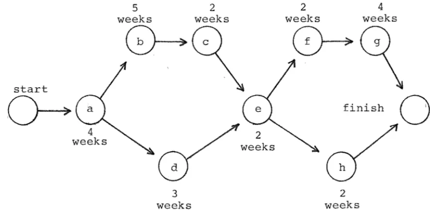
A second simple application appears in critical path analysis

(Hu, 1982). Here a chart is made indicating which subtasks rely on which other subtasks in a large scale overall task, and for each subtask there is a time required, or cost. Then the time required by the overall task will be the total time needed on the longest path through the network. For example,

if the task is building a house, a critical path analysis might reveal:

task time required must follow

a. design 4 weeks

b. site preparation 5 weeks a

c. foundations 2 weeks b

d. frame construction 3 weeks a e. frame erection 2 weeks c, d

f. roofing 2 weeks e

g. interior finish 4 weeks f

h. exterior finish 2 weeks e

This analysis can also be translated into the following diagram:

start

~

5 2

weeks weeks

~

3 weeks

weeks

2 4

weeks weeks

[image:13.597.82.525.580.797.2]

In this simple example the critical path is a-b-c-e-f-g for a total cost of 19 weeks. The longest path in such a situation can be found with a modified shortest path algorithm.

Another problem readily solved by shortest path algorithms is the maximum reliability problem. Consider a telephone based computer network, where each host to host connection (i,j) is independently subject to loss of information at some random but known rate Pij" To achieve reliable transmission of

important information between pairs of nodes it is desired to find the route of maximum reliability. By taking the "cost" of each connection to be -log(p .. ), the most reliable path

1]

can be easily found with the use of a shortest path algorithm.

1.3 page 10

1.3 Definitions and Notation.

The notation and terms used for various graph properties are well established, and a full description can be found in, for example, Bondy and Murty (1976), Even (1979), and Aho et al

(1974). In this thesis the following descriptions of graphs, networks, and the shortest path problem will be used. For amplification of any of these definitions the reader is referred to the books mentioned.

A directed graph G=(V,E) consists of a non-empty and finite set V of vertices and a finite multi-set E

=

{(u,v) :u,v in

v}

of edges. The size of the graph will always be described by the two parameters nand m, where n=IVI and m=IEI. The set V will often be numbered, V={v₁,v₂, ••• ,vn}' but no ordering

is implied by this; and for the sake of brevity the index will often be used to represent the vertex, so that

V={l,2, ••• ,n} and (i,j) represents the edge (v.,v.). In

1 J

all cases the meaning should be clear. Other terms for vertices and edges are sometimes used, notably the terms nodes for vertices and arcs for edges. For the purposes of shortest path calculation, the multi-set E can be reduced to a set of no more than n(n-1) edges by the deletion of all self loops (v,v) and the replacement of multiple edges connecting the same two vertices by a single edge. Thus, without loss of generality, it will be assumed that all graphs 90nsidered have m <= n(n-1), and have no self loops and no parallel edges.

For each edge e=(i,j), v. is the source and v. is the

1 J

destination, denoted srce(e) and dest(e) respectively. A Eath P from vertex u to vertex v is a finite sequence of k

edges {ei} such that srce(e

1)

=

u, dest(ek)

=

v, and for 1 < i <= k, dest(e.

1) = srce(e.). Then k is the length of

1- 1

the path. The empty path of length zero is also permitted, and links a vertex with itself. A path is simple if it contains no repeated vertices, so that any path P that is

uv

simple has length(Puv) < n, and the number of simple paths between any two vertices is finite. There may be an infinite number of non-simple paths between two vertices.

If there is a path from vertex u to vertex v, then v is

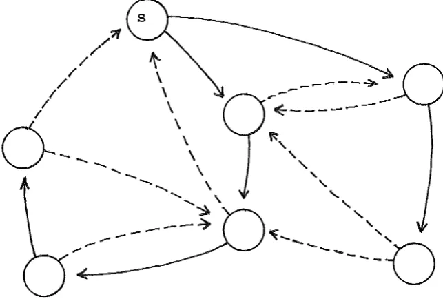
reachable from u. A vertex is always reachable from itself. If every vertex in a graph is reachable from every other vertex then the graph is strongly connected. For a strongly connected graph it will be the case that n <= m, since at least n edges must be present before every vertex can be

reachable from every other vertex. The graph of figure 1.3 is strongly connected.

[image:16.595.127.447.502.716.2]

1.3 page 12

For the purposes of shortest path calculations pairs (u,v) that are not present in E may be included in E as edges of arbitrarily large cost without affecting the computation, and thus it will be assumed without loss of generality that all graphs considered are strongly connected. That is, all graphs considered will have n <= m <= n(n-1). These

assumptions are in no way a restriction on the topology of the graph to be solved, as graphs that do not meet these requirements can be modified by a simple linear time preprocessing stage. The assumption that the graph is directed is also not a restriction, as undirected graphs

(such as that of figure 1.1) can be considered to be directed graphs, where each undirected edge (u,v) corresponds to two directed edges (u,v) and (v,u) of identical cost.

A cycle in a directed graph is a non-empty path Puu from a vertex u back to itself. An acyclic graph is a graph in which there are no cycles. The graph of figure 1.4 is acyclic.

[image:17.597.119.471.546.746.2]

A spanning tree rooted at some source vertex s in a strongly

connected directed graph G=(V,E) is a subset T of E

containing n-1 edges and such that every vertex in V is

reachable from s in the graph (V,T). A spanning tree will

always be acyclic; and between any two vertices in the

spanning tree there may be zero or one paths, never more. In

(V,T), if vertex u is reachable from vertex v, then v is an

ancestor of u, and u a descendent of v. The edges drawn

heavily in figure 1.5 form a spanning tree of the graph

rooted at vertex s.

"",

'

'

'

'

'

'

'

'

"' ... ___ ' ... o

--

....

_

Figure 1.5 -A spanning tree.

A network N=(G,C) is a directed graph G together with a real

valued function C defined on the edges of G, C:E -> R. For e

in E, the real number C(e) is the cost, or weight, of edge e.

If e=(i,j) then C(e) will also be denoted by C(i,j). The

concept of cost is extended in a natural manner to paths: for

path Puv = (e

1,e2, ••. ,ek) define C(Puv) = sigma(i=l,k)C(ei).

[image:18.595.126.448.356.573.2]

1.3 page 14

A shortest :eath from u to v is a path Puv such that C(Puv) is minimal over all possible paths from u to v. The number of edges in the path is immaterial; a path from u to v of

minimal number of edges will be referred to as edge-shortest. Edge-shortest paths in a graph can be found efficiently by a breadth first search procedure. If any path from u to v contains as a subpath a cycle of negative cost, then the minimum is not defined and there is no shortest path from u to v. If no path from u to v contains a negative cost cycle and v is reachable from u then a shortest path from u to v exists. Further, if there is a shortest path from u to v

then there is a shortest path that is simple, constructed by deleting all cycles from any non simple shortest path. This

is valid since no' cycle has negative cost. Thus, without loss of generality it may be assumed that a shortest path is simple. For a network N=(G,C), define the shortest path cost function LN to be the function LN:V X V -> R, where

LN(u,v)

LN(u,v) LN (u ,v)

=

=

:::: C(P )

uv

if there is a path from u to v with a negative cycle,

if there is no path from u to v, for some shortest path Puv

The subscript N will normally be dropped without ambiguity. In this thesis only cost functions C that are non-negative will be considered. Then for these cost functions there can

be no negative cycles, and the function L will also be entirely non-negative. This restriction is important; the algorithms discussed here are incorrect when applied to

general, algorithms that solve the unrestricted shortest path problem in the presence of negative edges are less efficient

than algorithms for the restricted problem where it is assumed that there are no negative arcs. Johnson (1973) considers the shortest path problem when the edge costs may be negative.

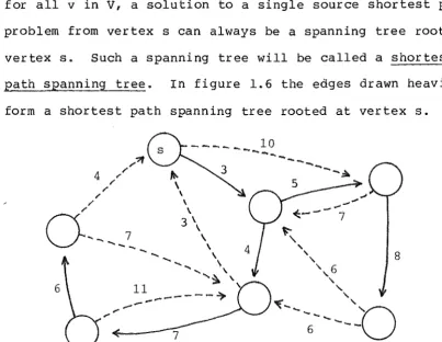
For any pair of vertices u and v let Puv be a shortest path from u to v. Then any subpath of Puv is also a shortest path, since if there was any shorter path connecting the two intermediate vertices, P _uv could be shortened, and would

not be a shortest path. Hence, supposing L(s,v) to be nite for all v in V, a solution to a single source shortest path problem from vertex s can always be a spanning tree rooted at vertex s. Such a spanning tree will be called a shortest Eath SEanning tree. In figure 1.6 the edges drawn heavily form a shortest path spanning tree rooted at vertex s.

6 11

---..!)o

--...

....

~\.

'

'

'

_{' 6}

'

'

_...

8

...

"(_, 'o

...._

..._

6

-Figure 1.6 - A shortest path spanning tree.

[image:20.597.82.485.372.683.2]

1.3 page 16

In the single pair problem (spp) there is one element in the list and a single shortest path is required; in the single source problem (ssp) there are n-1 elements in the list and each element is of the form (s,v) where s is some fixed

source vertex and v ranges over all other elements in V; and in the all pairs problem (apsp) the list contains n(n-1) elements, and shortest paths are sought between each pair of distinct vertices in the graph.

Primarily the results given here concern the all pairs problem, but many of the apsp algorithms discussed use a single source algorithm n times, once for each vertex in the graph.

The solution to a shortest path problem can also take one of three forms:

The numerical value of the cost of each shortest path may be required, that is, the appropriate values of the function L are wanted; or the cost of a shortest path together with an instance of a shortest path may be desired; or the cost of a shortest path together with a list of all possible paths that have that cost may be required.

The number of distinct shortest paths between two vertices may be exponential in n, requiring exponential time to list

them, so the third solution type is outside the current discussion, which is concerned with fast polynomial time algorithms. For the purposes of this thesis, a solution to the shortest path problem will consist of one representative shortest path for each pair of vertices in the problem.

programs presented here will typically only calculate

shortest path costs and not a shortest path, but in all

instances the algorithms are constructive and the programs

are easily modified so that a shortest path as well as the

shortest path cost can be recovered. The text associated

with each algorithm will describe the modifications needed to

recover the shortest paths; the programs themselves will

compute the function L over the required range and will not

include statements to record the information that would be

needed to build a shortest path spanning tree.

Closely linked to the all pairs shortest path problem is the

distance matrix multiplication (dmm) problem. Let

X= (x .. ) andY= (y .. ) ben by n matrices of real values.

1] 1]

Then the distance matrix multiplication problem requires the

calculation of the matrix Z

=

(z .. ) =X* Y, where

1]

zij =min{ xik+Ykj : O<k<=n }, that is, multiplication in the

distance matrix semi-ring (Aho et al, 1974). The link

between the apsp and the dmm problems will be discussed in

chapters two and six.

Of great interest is the running time of algorithms for

finding the solution to a shortest path problem. In all

cases analyses given here will be based on the random access

machine model (Aho et al, 1974) in which all arithmetic,

logical, and indexing operations take unit time. Such a

model frees the analysis from consideration of the actual

numeric values involved in any particular computation, and in

general it will be possible for the running times to be

described as functions of the graph parameters m and n.

1.3 page 18

operations it is convenient to use the concept of asymptotic growth rate, and the standard notation established by Knuth

(1976) is followed. Briefly,

f(n,m) = O(g(n,m)) when there is some constant k such that for all sufficiently large m and n, f(n,m) <= k*g(n,m)

f(n,m)

=

.(}.(g (n ,m)) when there is some constant k such that for all sufficiently large m and n, f(n,m) >= k*g(n,m) f(n,m)

=

9(g(n,m)) when f(n,m)

=

O(g(n,m)) and

f (n ,m)

=

,n(g(n,m))

f(n,m)

=

o(g(n,m)) when f(n,m)

=

O(g(n,m)) and f (n ,m) is not 9(g(n,m)).

For example, the function 3n3+sn2logn can be described as O(n3), 9(n3), fi(n2logn), and 3n3+o(n3).

Using this notation three more graph definitions are added: a family of graphs is sparse if m

=

O(n) for members of the family; dense if m

=

.().(nl+k) for any small positive k; and complete if m

=

n(n-1). In general these definitions will be misused, and a single graph (rather than a family of graphs) will be described as sparse if the number of edges is close to n, and dense if the number of edges is substantially greater than n. Planar graphs, with no more than 6n-12 edges, are the usual example of a family of sparse graphs.

Chapter three will concentrate on the precise number of

costs. These are normally the dominant components of the running time of any shortest path algorithm, and a precise bound on the number of these data operations is of interest from a theoretical point of view (Kerr, 1970}. Indexing and similar operations are not counted at all. The reason for making this distinction is that the indexing operations will always be on the same data types, namely integers in the range 1 to n, but the addition and comparison of path costs may be expensive operations; they may, for example, involve multiple precision floating point numbers. Counting the number of additions and comparisons on path costs for a

shortest path algorithm is similar to counting the number of comparisons required by a sorting algorithm, where again the cost of the indexing operations is ignored so long as they do not dominate the running time. These two operation types -addition and comparison of path costs - are called the active operations of the algorithm. Johnson (1973} has also used the

same classification of operations for shortest path algorithms.

The analyses given here will sometimes be for the worst case, where the maximum running time that can be required by any graph of n vertices and m edges is calculated, and sometimes average case, where the time given is an expected running time. For an average case analysis some assumption must be made about the probability of each possible input

configuration, and the running time given is an expected running time for the specified distribution of input

1.3 page 20

hand, the average case analysis predicts what is likely to happen on an input randomly selected from the corresponding probability distribution, but if the input network by bad luck happens to have some undesirable configuration for that algorithm then the running time might be greatly in excess of the expected value. Of the algorithms presented here, some are good in the worst case, and some are good in the average case; it will always be made clear which framework is being used at any time.

During the course of the research that resulted in this thesis many computational experiments on the different shortest path algorithms have been carried out. These

empirical results have in many places been used to support analytically derived bounds on the running time of

algorithms, and to compare two algorithms for operational use. To the interpretation of these results should be added a caveat - running times are volatile, and depend heavily on the architecture of the computer, the compiler and language used, the timing facilities provided by the operating system, and so on. Moreover, despite care to avoid such problems, there may also have been some unconscious bias in the

implementations. Bearing in mind these two points, all running times given should be regarded as loose indications of relative performance and not as a precise measures of absolute performance. On the other hand, empirical

another; the number of operations is an attribute of the

algorithm and not the implementation.

The following mathematical conventions will be used. All

unspecified logarithms will be to base 2; when natural

logarithms are required the function ln() is used. The

function log 2 n means (log (n)) 2 ; the function loglogn means

log(log(n)); and the function log*n is defined to be the

minimum integer i such that log(log( .. log(n) •. )) < 1, where

the logarithm is taken i times. The taking of a square root

will be abbreviated as sqrt(), and sqrt(n) and k*sqrt(n) will

be further abbreviated to sqrtn and ksqrtn respectively. The

function exp() indicates exponentiation base e (=2.72), and

the constant pi represents

1l

(=3 .14) . The symbol [] is used

to mark the end of a proof. A glossary of all mathematical

symbols and abbreviations appears after chapter seven.

The following lemma is sufficiently widely used in the

analyses that follow that it is worth stating in the

introductory section. Hereafter the result will be used

without explicit reference.

Lemma 1.1 Suppose that in a sequence of independent trials

the probability of success at each trial is at least p. Then

the expected number of trials until the first success is not

greater than 1/p.

Proof. This follows from the standard result for the

geometric distribution (Feller, 1968). []

It also also worth reviewing the properties of the heap data

structure (Floyd, 1962b; Williams, 1964; Floyd, 1964), as

1.3

discussed in this thesis, and their properties will be assumed rather than explicitly stated in each case.

page 22

A heap is an implementation the priority queue abstract data type (Sedgewick, 1983) with the properties that a heap of n items can be build in O(n) time; the minimum weight element in the heap can be identified in 0(1) time; any element can be deleted in O(logn) time; and elements can have their weight updated in O(logn) time. All of these bounds are for the worst case.

The normal implementation of an n element heap is as an

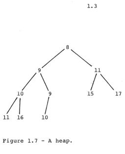
implicit binary tree stored in an n element array. In such an array the "father" of the element in position i is found in position (i div 2), and the two "sons" are in positions 2*i and 2*i+l. The heap property requires that an element not exceed in weight either of its two sons, meaning that the smallest weight element can be found at the root, stored in position 1. For example, the 10 element array

position: 1 weight: 8

2 3 4

9 11 10

5 6 7 8 9 10 9 15 17 11 16 10

satisfies the heap property, and represents the binary tree shown in figure 1.7. General purpose routines for

manipulating the heap elements to allow for updates of weight, insertion and deletion of elements, and heap

/8~

/\ l""

10 9 15 17

II

I

11 16 10

Figure 1.7 -A heap.

The Concise Oxford Dictionary (sixth edition, 1976) also provides a useful insight to the properties of a heap:

heap n. Group of things lying one on another; (in sing. or pl., colloq.) large number or quantity (a heap of people; there is heaps of time; have seen it heaps of times; he is heaps better); (colloq.)

battered old motor vehicle; knock or strike all of a heap; top, or bottom, of the~, (colloq.,fig.)

[image:28.595.110.366.50.365.2]

1.4 page 24

1.4 Overview of the Thesis.

The remainder of this thesis is organised as follows. Chapter two describes existing algorithms for finding shortest paths and also discusses lower bounds on the complexity of the problem, setting the scene for the new results.

In chapter three the precise number of active operations

required for a solution to the apsp problem is considered. A new priority queue data structure is developed, and leads to an apsp algorithm with an improved worst case bound on the number of active operations.

In chapter four the average running time for the all pairs problem is attacked, and a new algorithm that requires O(n2logn) expected running time on a wide class of random graphs is given, improving asymptotically the previous best result for this class of graph from O(n2lognlog*n). The chapter includes experimental results that show that the new algorithm is fast, and suitable for operational use.

Chapter five discusses the implementation of the algorithm of chapter four, and i t is shown that two apparently good

Chapter six is concerned with distance matrix multiplication, and a hybrid algorithm for this problem that on some families of random matrices runs significantly faster than any other known algorithm is presented. Also described is a

probabilistic algorithm for distance matrix multiplication that has worst case running time o(n3), and for some class of random matrices, good probability of calculating the optimal distance matrix product.

page 26

CHAPTER TWO EXTANT RESULTS.

2.1 Upper Bounds and Algorithms.

Worst case analysis.

The traditional algorithms for finding shortest paths have all been good in a worst case sense, and this area is

examined first. The earliest approaches to the apsp problem were based on distance matrices. If the cost function C and the shortest path function L are considered as distance

matrices, then L is the closure of C in the plus-min semiring (Aho et al, 1974), and so has the property that C

*

L

=

L, where

*

represents distance matrix multiplication. Provided that the network contains no negative cycles, this closure can be found by repeated squaring of (C+I), where I is a distance identity matrix. This is because no shortest path

n

need be more than n edges long, so that L

=

(C+I) . To

raise a matrix to the n'th power will require ceiling(logn) repeated squarings; and by a straightforward method each squaring will require O(n3) time. This then gives an

O(n 3 logn) time algorithm for the apsp problem, one of the earliest results.

Rearrangement of the calculation order for the inner products was the key to the O(n3) apsp algorithm given by Farbey et al

with the order of the "multiplications" within each inner product rearranged and again the most recent values always used.

Furman, Munroe et al have given the theorem, presented fully in Aho et al (1974), that distance matrix closure is

computable in O(T(n)) time if and only if distance matrix multiplication is also computable in O(T(n)) time, provided that T(n)= fL(n2) and T(n)=O(n3). In removing the O(logn) overhead required by repeated squaring this result has prompted many authors to attack the distance matrix multiplication problem.

First to succeed with an o(n3) distance matrix multiplication algorithm was Fredman (1975, 1976). He showed that O(n2"5) additions and comparisons on path costs were sufficient for the multiplication, but was unable to give a general

algorithm that required this running time. Fredman then went on to show that his technique could be exploited "mildly", and was able to give an O(n3(loglogn/logn)1

1

3) algorithm, which is o(n 3 ). However this algorithm is rather complex, and no implementation of it has been reported. It seems likely that extremely large problem sizes would be required before the method could become operationally competitive. For

example, the function 2n3(loglogn/logn)1/ 3 first becomes less than n3 when n=244 , and it seems not unreasonable to expect a constant factor of at least 2 for Fredman's method when compared with Floyd's method. Even at one trillion

2.1 page 28

Yuval (1976) gave a transformation involving exponentiation

and l~arithms that allows distance matrix multiplication to

be encoded into matrix multiplication over the real field. This then leads to an O(nb) algorithm for the apsp problem, where b is the complexity of matrix multiplication, currently approximately 2.5 (Schonhage, 1981). However critics have pointed out that to effect this scheme, even when the path costs are integers, very high precision real arithmetic is required, and that the true complexity is exponential

(Moran, 1981).

Because of this criticism, Fredman's o(n 3 ) result is

generally acknowledged as being the current worst case upper bound for distance matrix multiplication, and hence for the apsp problem on a complete graph.

The result of Munroe and Furman applies similarly to the problem of finding transitive closure in the Boolean

semi-ring. In that semi-ring, boolean matrix multiplication can be carried out in O(n 2 · 81 ) time using the technique of Strassen (1969). However this approach cannot be extended to

the distance matrix semi-ring, as it requires an inverse for the "min" operation. In the distance semi-ring, for arbitrary elements a there is no x such that min( x,a )

=

infinity.

Direct "graph" approaches to shortest path problems have also yielded good algorithms. Dijkstra (1959) gave an O(n2)

(1983) chapter 7) to give a running time of O(mlogkn), where k=max(m/n,2). For dense graphs this running time is O(m), which for the single source problem is optimal; for sparse graphs the behaviour is O(nlogn). Recently Fredman and Tarjan (1984) gave another implementation of Dijkstra's algorithm, using a Fibonacci heap, which runs in O(nlogn+m) time, a slight improvement over Johnson for graphs that are neither sparse nor dense. However all of these algorithms will work only if there are no negative arcs. If negative arcs are present then an O(nm) preprocessing step is needed before these algorithms can be used (Johnson, 1973). This makes them expensive for the single source problem, but the step is only required once, even if n single source solutions are to be combined to make an apsp solution. Using the

approach of Fredman and Tarjan, Dijkstra's algorithm can be used to solve the unrestricted apsp problem in O(n2logn+mn), which is O(n 3 ) on a complete graph.

These worst case bounds for the apsp problem are given in the table below.

algorithm year bound

Dijkstra 1959 O(n3)

Floyd 1962 0 (n3)

Johnson 1973 0 (nmlog kn), k=max(m/n,2) Fredman 1976 O(n (loglogn/logn) 3 1/3 ) Yuval 1976 0 (n ) , b=2.5 b

Fredman, Tar jan 1984 O(n logn+nm) 2

2.1 page 30

On complete graphs only the "impractical" algorithms of Fredman and Yuval have running times o(n3).

There have been many other shortest path algorithms given in the literature that have not been listed here. Among them are algorithms by Dial (1969), who used a bucket sort

technique to make an efficient implementation of Dijkstra's algorithm when the edge costs are all integers from some small range; Dantzig (1960), whose algorithm is similar to that of Dijkstra and will be discussed in detail in

section 4.1; Pape (1980) who uses an interesting heuristic to achieve a fast algorithm; and so on. Dreyfus (1969) gives a survey of early work and Mahr (1981) a more recent summary; the references section of this thesis lists a number of other papers.

Average case analysis.

Since 1972 there has been a great interest in apsp algorithms that have a good average case running time. Spira (1973)

pioneered this area with an algorithm he derived from

Dijkstra's and Dantzig's O(n2) time single source algorithms. By using a heap data structure, and a pre-sort to order the costs on the edges from each vertex, he was able to give an algorithm that requires O(n2log2n) time on average when the edges costs are independently drawn from any fixed but

arbitrary random distribution. His method involves the use of an O(nlog2n) single source algorithm for each of n

sources, but is not suitable for a single source problem

Corrections were made to his presentation by Carson and Law (1977), and Bloniarz, Meyer and Fisher (1979) formalised his idea of a random graph and also corrected his algorithm.

Subsequently his algorithm has been improved a number of times, with all of the improvements still using the same paradigm (Takaoka and Moffat, 1980; Bloniarz, 1980; Frieze and Grimmett, 1983). The table below lists the average

running times for the members of this sequence of algorithms; the algorithms themselves will be examined in greater detail in chapter 4. One of the main results presented in this thesis is the last algorithm listed in the table, which has average running time of O(n2logn).

algorithm year average case worst case

Dijkstra 1959 0 (n3) 0 (n3)

Dantzig 1960 0 (n3) 0 (n3)

Spira 1973 O(n log n) 2 2 O(n logn) 3 Takaoka, Moffat 1980 O(n lognloglogn) 2 O(n3logn) Bloniarz 1980 O(n lognlog*n) 2 O(n3logn) new algorithm 1985 O(n logn) 2 O(n3)

Table 2.2 - Average running time for apsp algorithms.

2

Frieze and Grimmett (1983, 1985) have also given an O(n logn) average time algorithm for the apsp problem, but their method is suitable only for a narrow class of probability

2.1 page 32

All of these methods rely on n successive iterations of a

single source algorithm, and require that the edge costs be

non-negative. The preprocessing step mentioned earlier as a

way of handling negative cost edges is not applicable, as on

a complete graph the preprocessing time would be 9(n3),

2.2 Lower Bounds.

An upper bound on the complexity of a problem is usually

shown by giving an algorithm that solves the problem and runs in some time T(n); this is sufficient to establish T(n) as an upper bound for the problem. On the other hand, lower bounds are much harder to develop. Apart from the so called

"trivial" bounds, where the number of inputs that must be examined by any algorithm and the number of outputs that must be produced are counted, there is no general technique for establishing lower bounds, and in general non-trivial lower bounds are scarce.

A lower bound B(n) on the complexity of a problem means that every algorithm that solves the problem must require at least B(n) steps for some input sized n. Because of the universal quantification over algorithms, both those invented and those not yet invented, lower bounds are normally established

2.2 page 34

this section briefly surveys the different computational models in which lower bounds have been given for the apsp problem.

The most restrictive model is that in which only operations + (plus) and min are permitted, and the operations must be

performed in straight-line order, that is, by a program that executes assignment statements only and has no branching based on the relative values of the input variables

(Kerr, 1970). Johnson (1973) has shown that in this

framework 2n(n-l) (n-2) active operations are required, making Floyd's algorithm optimal.

If the straight line requirement is removed to allow

branching, but the operations still restricted to plus and min, then Fredman's demonstration that O(n2"5) operations are sufficient (Fredman, 1976) is valid, meaning that the lower bound cannot exceed this. Yao at al (1977) attempted to show that the lower bound in this decision tree framework was 9(n 2logn) using information theoretic techniques, but their attempt was dismissed by Graham et al (1980), who showed that the only lower bound that could be established by that

If the costs may be treated as quantities over the real field, with subtraction, multiplication, and division

permitted in a decision tree model, then only trivial lower 3 bounds are known; it is in this area that Fredman's o(n ) algorithm lies. Again there is a wide gap between known upper and lower bounds.

If arbitrary precision real multiplication can be permitted as a unit operation, along with exponentiation and logarithm taking, then the results of Yuval (1976) and others (Romani, 1980; Moran, 1981) can be considered to be upper bounds in this still more liberal arena. Being based on matrix

multiplication, their methods are straight line.

These results are summarised in the following table:

arena

straight line, plus min only

dec is ion tree, plus min only

decision tree, real arithmetic

arbitrary precision real arithmetic

lower bound

2n (n-1) (n-2) Johnson 2 en Graham trivial trivial

upper bound

2n (n-1) (n-2) Floyd

Floyd, Dijkstra, et al

3 l/3

O(n (loglogn/logn) ) Fredman

Yuval, et al

Table 2.3 - Lower bounds for the apsp problem.

[image:40.595.99.524.448.709.2]

2.2 page 36

room for the development of either faster algorithms or sharper bounds or both.

For the single source problem, the situation is reversed. Here it has been shown by Spira and Pan (1975) that on a complete graph (n-1) (n-2) active operations are required, even in a liberal decision tree computational model with plus, min, and subtraction permitted. Here there is little scope for improvement over the algorithm of Dijkstra, and it seems likely that O(nlogn+m) running time cannot be improved for conventional uni-processing computer hardware and

arbitrary graphs.

If parallel architectures or distributed processing

CHAPTER THREE

A GOOD WORST CASE ALGORITHM.

3.1 Background.

This chapter concentrates on the worst case behaviour of apsp algorithms; in particular, on the precise number of active operations that are required when calculating a solution to an apsp problem.

Fredman (1976) showed that O(n2·5) active operations were sufficient for a solution to the apsp problem, but did not give an algorithm realising this bound in terms of running time as well as operations. If his idea is implemented, an algorithm that requires O(n2·5) active operations and 9(n3·5) running time will result; to date there has been no

successful attempt to reduce the running time of this technique to the o(n3) level while still retaining the O(n2· 5) bound on active operations. The first result

presented in this chapter is a new "greedy" algorithm that when coupled with an appropriate priority queue requires n3

+

o(n3) additions and comparisons on edge costs, and O(n3) running time in the worst case. Thus, although Fredman's result means that n 3 cannot be claimed to be a best upper bound on the number of active operations, an O(n 3 ) worst case time algorithm is given that requires only n3

+

o(n3)

operations, which Fredman did not do.

3.1 page 38

path costs as real numbers and work within the real field rather than the plus-min semiring. So although he attained o(n 3 ) running time, he did so outside the plus-min semiring structure that is considered here. Within the semi-ring the only operations permitted on path and edge costs are addition and binary min operations, and it is these that are counted as being the active operations of an algorithm.

In an early paper Dantzig (1960) gave an algorithm for the single source problem (see section 4.1) which requires O(n2+t(n)) time, where t(n) is the time needed to sort the edge lists of the graph. For a dense graph, t(n)

=

O(n2logn) and the algorithm will require O(n 2logn) time for the single source problem, an inferior result to the ssp algorithm of Dijkstra. However, application of Dantzig's technique to the apsp problem results in an O(n3) algorithm, as the cost of sorting the edge lists is shared over all sources. Moreover, not noted by Dantzig is that a careful implementation of his technique results in an algorithm that solves the apsp

problem using n3 + O(n2logn) active operations. This result has been overlooked by many authors - for example Yen (1972)

(see also Williams and White, 1973) reports an implementation of Dijkstra's algorithm that requires 1.5n3 active

operations.

Because of this result by Dantzig, the greedy algorithm presented in the first part of this chapter is of interest mainly as an exercise in algorithm design. An old technique

queue itself that is the main result of this chapter. This new priority queue can also be applied to Dijkstra's

algorithm, giving again an algorithm that requires n3

+

o(n3) active operations on a complete graph. However this

implementation also gives an O(mn) bound on operations and running time on graphs that are dense but not complete, thus improving upon the result of Dantzig.

Tomizawa (1976) also did some work in this area; he gave an implementation of Dijkstra's algorithm that requires

3mn

+

n2sqrt(2nlog(2n)) active operations in the worst case to solve the apsp problem. The final implementation of Dijkstra's algorithm given here is superior to Tomizawa's bound for both complete graphs and graphs that are dense but not complete.

For practical implementations none of these methods with good worst case behaviour can compete with the average case

methods of Spira (1973) et al, and the O(n3) algorithms are of interest from a theoretical rather than an operational point of view. Moffat (1983) gives a computational survey of apsp algorithms that demonstrates that the fast average case

3

methods are practically faster than any of the O(n ) methods, and, presumably, that of Fredman, although no implementation of his algorithm has been reported. The experimental results given in section 4.5 of this thesis also show this practical superiority.

3.2 page 40

3.2 The Greedy Paradigm.

The new method is based on the greedy design paradigm, and was initially given in an undeveloped form in (Moffat, 1979). There the best time bound that was obtained was O(n3logn). In this presentation Kruskal's (1956) algorithm for finding a minimum cost spanning tree is briefly stated as an example of the paradigm, and is then extended to the all pairs shortest path problem.

Kruskal's algorithm.

Kruskal's algorithm for finding a minimum cost spanning tree T in an undirected network is described in outline below. The method is described in detail by Tarjan (1983).

procedure kruskal ; begin

mark all edges in E unchecked ;

T := {} ;

while there are edges in E that remain unchecked do begin

let (u,v) be the least cost unchecked edge ; if (u,v) can be used in the spanning tree then

T := T + {(u,v)}; mark (u,v) checked ; end

end {kruskal}

Algorithm 3.1 - Kruskal's Algorithm.

The algorithm is greedy in that, to build a global minimum of cost, each step involves finding a local minimum - the

Application to shortest paths.

An algorithm for the all pairs shortest path problem can be

constructed from a similar skeleton. For any pair of vertices

u and v the cost of the shortest path from u to v must be

either the cost of the direct edge (u,v) or the cost of an

indirect path through some intermediate vertex p. In this

latter case, because all edge costs are non-negative, neither

L(u,p) nor L(p,v) can exceed L(u,v), where L is the shortest

path cost function defined in section 1.3. Shortest paths

can thus be created by checking paths in ascending order of

cost, and, as each path (u,v) is checked, searching for

longer paths that might in turn have their cost reduced if

(u, v) is used as part of an indirect path. All edge costs are

non-negative, so that once checked a path or edge cannot have

its cost reduced, and re-scanning is not necessary. Thus it

suffices for the algorithm to make a single pass over the

pairs of vertices of the graph, checking each edge once. In

the following program, the array "pcost" records tentative

shortest path costs:

procedure greedy-apsp

be~ in

\initialisation}

for all (u,v) in V X V do

mark (u,v) unchecked and set pcost[u,v] := C(u,v)

for all u in

v

do

mark (u,u) checked and set pcost[u,u] := 0 ;

{main processing loop}

while there are unchecked (u,v) in V X V do begin

getrnin: let (u,v) be such that pcost[u,v] is minimal over all unchecked pairs (u,v)

check: for all a,b in

v

X

v

do

attempt to reduce pcost[a,b] using (u,v) as one part of an indirection mark (u,v) checked

end ;

end {greedy-apsp} ;

3.2 page 42

The invariant relating the array "pcost" and the shortest path function L is as follows. If a pair (u,v) has been checked, then pcost[u,v]

=

L(u,v), and the correct shortest path cost is recorded. If, on the other hand, (u,v) has not been checked, then pcost[u,v] is either the cost of the best tentative path from u to v that consists of two checked

paths, or the original cost of the edge (u,v), whichever is smaller. In all cases pcost[u,v] will be no greater than C(u,v), the original cost of the edge.

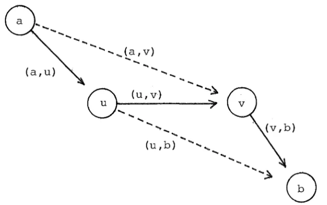
The step "check:", searching for paths that might be

shortened by the use of (u,v), can be more efficient than a 2

[image:47.598.124.459.457.667.2]

simple search through all of the as many as n unchecked paths:

...

...

...

...

... (a,v)

... ...

...

...

...

....

~

0}~u,v)

...

...

...

(u, b) ...

...

Figure 3.1 - Checking (u,v).

...

... ...

).

(a,v) need only be tested if (a,v) has itself not already been checked and (a,u) has been checked. If the first of these two additional conditions is not met then pcost[a,v] has already been assigned the optimal value L(a,v), and the test is pointless. If the second condition is not met then the test can be deferred until pcost[a,u] has been given a final value at the time when (a,u) is checked; this delay has the advantage that the test might be avoided entirely if

L(a,v) < L(a,u) and (a,v) is checked first. A similar pair of conditions apply to pairs (u,b) that might have their pcost updated. The following procedure describes this

checking strategy, and a call to this procedure replaces the loop marked "check:11

of procedure greedy-apsp.

procedure check-pair ( u,v ) ; begin

for a in V do

if (a,u) is checked and (a,v) is not checked then begin

newcost := pcost[a,u]

+

pcost[u,v] if newcost < pcost[a,v] then

update pcost[a,v] to newcost end ;

for b in V do

if (v,b) is checked and (u,b) is not checked then begin

newcost := pcost[u,v] + pcost[v,b] if newcost < pcost[u,b] then

update pcost[u,b] to newcost end

end {check-pair} ;

Algorithm 3.3 - Checking (u,v).

An implementation of Kruskal's algorithm requires some data structure for ordering the edges by cost, and the same is true of greedy-apsp. However, with greedy-apsp the data structure used must be capable of handling updates to the weights of the elements stored, an operation not required by

3.2 page 44

queue structures that are typically used for an

implementation of Kruskal's algorithm, such as a sorted list or a binary heap, are not suitable. In the initial

description of the greedy-apsp method (Moffat, 1979), a binary heap was employed, leading to a bad O(n 3logn) worst case running bound. Here the implementation uses a different priority queue - section 3.3 describes a data structure that enables successive minima to be found in O(sqrtn+logn) time each, even allowing for the updates on path costs that will be required. Given such a data structure, each execution of the main while loop of greedy-apsp can be seen to take

O(n+sqrtn) time, and the whole algorithm will require O(n3) time in the worst case.

If the shortest paths are required, a simple modification can be made to the algorithm so that each time an entry of array "pcost" is updated the intermediate vertex that successfully reduced the path cost is also recorded. At the conclusion of the algorithm the shortest paths would then be recovered as well as the shortest path costs.

Correctness of algorithm greedy-apsp.

The following lemmas identify the ideas required to show the correctness of the method.

Lemma 3.1 For all pairs (u,v) in V X

v,

no changes to the value of pcost[u,v] will take place after (u,v) is checked. Proof. From the guards of the program text. []

Proof. From the guards of the program text. []

Lemma 3.3 The costs of the pairs checked at each iteration of the main while loop form a non decreasing sequence.

Proof. Suppose (u,v) is checked at some iteration. Then the new values assigned by any updates that take place during the call "check-pair(u,v)" will be pcost[u,v] plus some

non-negative quantity. On the other hand, all paths that are not updated have path values not less than pcost[u,v] anyway. In either case all remaining unchecked pairs after (u,v) is checked have pcost values not less than pcost[u,v]. []

Corollary 3.4 Suppose that (x,y) is such that, at the

conclusion of greedy-apsp, pcost[x,y] < pcost[u,v]. Then at the time when (u,v) is checked, pair (x,y) will have already been checked. []

Theorem 3.5 The program greedy-apsp correctly computes shortest path costs. That is, at the conclusion of

greedy-apsp, pcost[u,v]

=

L(u,v) for all (u,v) in V X V.

Proof. From the constructive nature of the algorithm, a path exists from u to v of cost pcost[u,v], so

L(u,v) <= pcost[u,v] for all u and v. However, suppose for some pair (u,v) that L(u,v) < pcost[u,v], meaning that there is some path from u to v of cost strictly less than

pcost[u,v]. To be specific, let (u,v) be the first path checked for which, at the conclusion of the algorithm,

L(u,v) < pcost[u,v]. Then since pcost[u,v] is initialised to C(u,v) and is non-increasing, the path represented by L(u,v) must contain at least one intermediate vertex. Let this

intermediate node be vertex p. All edge costs are

3.2 page 46

less than pcost[u,v]. From this it follows that

L(u,p) = pcost[u,p]; that L(p,v) = pcost[p,v]; and thus that (corollary 3.4) both were checked before (u,v). Assume,

without loss of generality, that (p,v) was checked after

(u,p), at iteration t of the main while loop. For pcost[u,v] not to have been set to pcost[u,p] + pcost[p,v] at iteration t would require that either (u,v) had already been checked, in which case pcost[u,v] <= pcost[p,v] (lemma 3.2), or that pcost[u,v] was already less than pcost[u,p] + pcost[p,v]. In both cases, pcost[u,v] cannot subsequently have increased

(lemma 3.2) nor can pcost[u,p] or pcost[p,v] have decreased (lemma 3.1), and this gives the desired contradiction. Thus it cannot be that L(u,v) < pcost[u,v]. []

Analysis of active operations.

Given that the priority queue data structure can be

implemented within the claimed bounds of 0(1) time per update and O(sqrtn) time and data operations per "getmin" operation, the running time of the whole algorithm is easily seen to be O(n3), meaning that the number of active operations must also be O(n 3 ). To precisely count the number of operations

Figure 3.2 -A triple of vertices.

Lemma 3.6 In any triangle of vertices such as is depicted in figure 3.2, of the two paths (s,a) and (s,b) out of vertex s, the checking of the second will never cause a test on that checked first.

Proof. The guards in the text of procedure check-pair ensure that no pair will ever be tested after it is checked. []

Note that even in the case of paths of equal cost, one must be checked before the other.

Lemma 3.7 Over all calls to procedure check-pair there will be at most n(n-1) (n-2) active operations on path and edge costs.

Proof. There are n vertices, each of which is the source in (1/2) (n-1) (n-2) triangles of the form shown in figure 3.2. Lenuna 3.6 bounds the number of tests per triangle at 1, and each test requires one comparison and one addition. []

3.3 page 48

3.3 Priority Queue Implementation.

The algorithm described in section 3.2 requires a priority queue. By recognising and exploiting the relationships among the edges in the queue that get updated, it can be

implemented efficiently using a two level approach.

The upper queue.

The top level of the data structure is a binary tournament tree (Knuth, 1973b) of n entries, one for each vertex in the graph. Each of the entries represents the best candidate path, in terms of cost, of the unchecked paths that are

incident at that vertex. That is, each entry represents the least cost unchecked path either incoming or outgoing at that vertex, of which there may be as many as 2(n-l). As a

consequence, each unchecked pair (u,v) appears in two places in the data structure - once in the lower queue as an

incoming path of vertex v, represented in the upper queue by the candidate for v, and once in the lower queue of vertex u, as a path outgoing from u. This structure for the upper

/ /

f

/'

0

lower queue for vertex u

~

entries

Figure 3.3 -The upper queue.

'

' '

'

in queue

"

"

'

upper queue

--~

lower queue for vertex v

for path (u,v)

Because the cost of each path is non-increasing, it is not necessary for the entry in subqueue u for (u,v) to record the same cost as that in subqueue v, so long as one of the two records the most recent value of pcost[u,v]. This is safe since the priority queue "getmin" operation will return the smaller of the two different values first, which is always the most recent value. When pcost[u,v] is updated, it does not matter which of the two entries in the lower queues is altered. This freedom of choice can be used to good effect.

[image:54.595.99.521.85.404.2]

3.3 page 50

of choice, in the upper queue by the candidate for v. Thus when (u,v) is being checked all updates can be confined to two of the lower queues, so that in the upper queue only two of the entries will change between successive getmin

operations. Pair (u,v) will itself be deleted from the entire data structure, but this change is also restricted to the same two candidates in the upper queue. Thus each execution of the main while loop, involving a "getmin" operation and a call to procedure check-pair, will require only O(logn) time and O(logn) comparisons of path costs in the upper queue.

Construction of the upper queue will require O(n) time, once the initial candidates from the lower queues have been

established. Over the whole algorithm greedy-apsp, the upper queue will require O(n2logn) time and O(n2logn) active

operations.

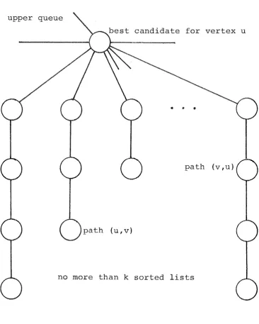
The lower queue.

upper queue

best candidate for vertex u

.

.

'

path (v,u)

path (u,v)

no more than k sorted lists

Figure 3.4 - The lower queue for vertex u.

Pointers are kept to the location of each element so that any element can be deleted in 0(1) time. Such a deletion may

[image:56.595.107.474.94.552.2]

3.3 page 52

The initial construction of each lower queue requires that the list of 2(n-l) edges incident at a vertex be sorted and formed into a single doubly linked list; this will take for each subqueue O(nlogn) time and comparisons on edge costs.

From lemma 3.3 it is known that the paths checked form a non-decreasing sequence, meaning that for each vertex a sorted list of checked outgoing paths and a sorted list of checked incoming paths can be maintained without additional data operations. If these lists are used as the ordering of the

''for" loops of procedure check-pair then the sequence of new paths resulting from successful tests will also be in

non-decreasing order, since in effect a constant is