Detecting the pain evoked P300 in single trials: a comparison of template based models

Detecting the pain-evoked P300 in single trials: a

comparison of template-based models

Master Thesis

Dominic Portain

Dr. Rob van der Lubbe (Department of Cognitive Psychology and Ergonomics) Dr. ir. Jan R. Buitenweg (Department of Biomedical Signals and Systems)

Abstract

Introduction

Event-related potentials (ERPs) have traditionally been studied under the assump-tion that each measurement contains a staassump-tionary part (stable in relaassump-tion to the stimulus event) and a non-stationary part (varies independently from the stimulus event). From the assumption that ERPs remain stable over time if all environmental factors stay constant, the stationary part has been considered far more valuable than the non-stationary part. This assumption made it acceptable to sacrice non-stationary information, in order to improve the accuracy of stationary information. Partly due to this paradigm, the widely used pro-cedure has been to examine the average of several ERPs - instead of examining single trial ERPs. Event-related averaging has mainly been used to raise the - very low - signal-to-noise ratio (SNR) in single trials. However, continuing technological advances caused the physical noise to decline during the decades. This development is met by advancements in analysis algorithms that become more eective at separating the signal from background activity.

History of the EML

One of these algorithms, the Enhanced Maximum Likelihood (EML) method, will be the main subject of this study. Initially, Pham et al. proposed (Tuan, Möcks, Köhler and Gasser, 1987) and evaluated (Möcks, Köhler, Gasser and Tuan, 1988) a method for estimat-ing the latency of ERP components in stimulus-locked trials. This method, initially called iterative Fisher scoring, relies on two references: a template contained an idealized signal with the expected ERP component, and a noise prole provided an idealized representation of real-world background activity. Template-based models are considered more robust than feature-based models (which search for signicant features such as lines, slopes or edges) when encountering strong sample variance. The principle of a template approach is based on a comparison between the template and a measured sample ERP. In addition to the signal, the sample also contains background noise:

wheretdenotes the single time points of the analyzed waveshape (from 1 toT),rj(t)is the

activity measured at time t,s(t) is the constant event-related signal, and ej(t) is the noise

signal. This simplied model assumes that the signal s(t) is invariant between trials and

uncorrelated to the noise set.

Woody's method. Woody's method (Woody 1967) uses statistical correlation to com-pare between sample and template (see gure 1). The time oset between template and sample is shifted until the correlationρs,r becomes maximal:

ρs,r =

cov(s(t+τj), rj(t))

σsσr

Relying on a full-length template makes Woody's method very robust to noise contamination and localized artifacts (Jaskowski and Verleger, 1999). Smulders, Kenemans and Kok (1994) improved this method when nding that using covariation instead of correlation resulted in slightly increased performance.

Figure 1. Illustration of Woody's method. A low-noise template (left) is cross-covariated against a noise-contaminated sample (middle). The cross-covariation is yielded as function of time oset between sample and template (right). Note that, in the central chart, the noise-induced peak at 1700ms yields a much smaller covariation value than the correct one at 280ms - despite its larger amplitude.

no overlap between the frequency distributions of signal and noise. Although the ML also relies on an idealized signal template, it employs a fundamental improvement over Woody's method (Jaskowski and Verleger, 2000): acknowledgment and usage of background noise as a data source. The simplied model is Fourier-transformed to t the frequency-domain ML:

Rj(ω) =S(ω)−iωτj+Ej(ω),

whereω = 0,(2_Tπ),(4_Tπ), ... describes a nite set of frequencies, and capital letters stand for Fourier transforms of time-domain data. There are two data sources available, one with the idealized signalS(ω) and one that describes the underlying noise sweepNj(ω):

Nj(ω) = (S(ω)−iωτj −Rj(ω))

The unknown latencyτj can be estimated by maximizing1the log likelihood function LLF(for

a complete description, see Tuan et al., 1987):

maxτj

Nj(ω)

LLF(S(ω)−iωτj−_R

j(ω))

Enhanced Maximum Likelihood method. The enhanced ML (EML) removes a limita-tion of the simplied signal model: the underlying signal is no longer amplitude-invariant. To allow for changing waveform amplitude between trials, Jaskowski and Verleger (1999) added an optimization variable to the previous model:

Nj(ω) = (ajS(ω)−iωτj−Rj(ω)),

1_{This maximization problem was originally solved by iterative Fisher scoring, providing the name for this}

whereaj stands for the amplitude of the jth trial. Accordingly, the maximization problem

uses a second parameter:

maxτj,aj

Nj(ω)

LLF(ajS(ω)−iωτj −Rj(ω))

Jaskowski and Verleger (2000) reported severe problems when using the iterative Fisher solver, which allowed them to maximize both variables simultaneously. Iterations failed to converge to a stable result or converged in a local maximum. Preliminary analysis over our dataset indicated that there was no correlation between both parameters, allowing us to use a two-step direct approach:

maxajmaxτj

Nj(ω)

LLF(ajS(ω)−iωτj−Rj(ω))

The original paper relied on Fourier-transformed data for the EML calculation, a compro-mise2 _{between temporal resolution and frequency bandwidth (see Jaskowski and Verleger,}

2000: ML method). This approach limited the analysis to the principal (low-frequency) components of the P3 waveform, and severely reduced the accuracy of the latency estima-tion results. To resolve this compromise and maximize EML accuracy and performance, we adapted the algorithm to accept wavelet-transformed data:

maxajmaxτj

X

f

log(Inoise(f))

LLF(ajsf(t+τj)−rf,j(t))

,

where f denotes a single frequency component in the wavelet-transformed domain. Phase information and trial dependency were removed from the noise sweepNj(ω), resulting in a

general noise intensity spectrum Inoise(f). The logarithmic scaling of the noise prole was

required to match the LLF output.

2_{Jaskowski and Verleger (2000) used a Fourier bandwidth of 10 frequency components, corresponding to}

Previous study

Jaskowski and Verleger (2000) compared three distinct computational models in their performance to detect P3 peak latencies. All models were based on earlier studies, but had not yet been used in P3 detection. In addition to Woody's method and the EML, peak picking was also used in the performance comparison. Peak picking scans the ERP for the largest positive amplitude and returns the time position of this peak. The authors con-trolled P3 amplitudes, latencies and background noise levels using pseudo-real simulations (Gasser, Möcks and Verleger, 1983; Möcks, Gasser and Pham, 1984). Accuracy deteriorated strongly with increasing noise levels. The EML produced the most accurate results by a small margin. The authors also stress the limitations of a template-based approach, mainly due to the rigid signal model.

Study goals

The current paper is an update of the study performed by Jaskowsi and Verleger (2000). The rst goal was to establish the validity of our EML implementation. While the previous study mainly focused on the determination of P3 latency, this paper extended the focus to include peak amplitude estimation (as suggested by Jaskowski and Verleger, 1999). As result of more recent research eorts (introduced by Falkenstein, Hohnsbein and Hoormann, 1994; for an overview see Quevedo and Coghill, 2007; Polich, 2007), the P3 event was shown to consist of two independent components: the classic P3b, and the more physiologically-focused P3a. Pain stimuli are known to cause an unusually strong P3a am-plitude. This eect is benecial for the detection of small signals in single-trial analysis. In contrast to the traditional P3 production by oddball task (Donchin, Ritter and McCallum, 1987), the P3a creation is unrelated to the current task (Polich, 2003; Polich, 2007). Com-ponent onset is earlier and more intense when stimulus intensity is increased (Bromm and Scharein, 1981). Because of these features, we used pain-evoked P3a samples exclusively.

measurements were required (which didn't exist in our data) we adapted this procedure to create noise sweeps.

The validation procedure consisted of two parts: the articial condition and the real-istic condition. Focus lay on the inuence of noise contamination on the estimated results. The rst - articial - condition examined the models' performance under ideal conditions, using a pseudo-real dataset that contained only one prototypical P3a waveform (sampled from an illustration in Polich, 2007). The second part introduced ERP variation between trials. In the realistic condition, the pseudo-real dataset contained subject-specic grand-average ERPs.

The two traditional models (Peakpicking, Woody's method) were expected to perform similarly to those described by Jaskowski & Verleger (2000), showing a close link between noise contamination and model error rate. The two new models (ML, EML) were expected to yield more accurate results than the two traditional models, and to perform at least as well as the implementations described in the previous study.

Method

Data recording

The study included data from 16 subjects (students between 19 and 25 years) who produced 102 trials during each of four experimental blocks. The data for this study was created and provided by Blom and Braukmann. Participants received pain stimuli and responded according to stimulus intensity and location. Subcutaneous electrical stimulation on each forearm delivered the stimuli. Stimulus intensity was controlled by varying the number of impulses (spaced at 5ms) per pulse train. In the data for our rst analysis, there were two intensity conditions, high and low. We used only data from the high condition. The dataset for our second analysis contained responses to increasingly intense electrical stimuli. We used only trials that exceeded the subjects' pain threshold.

The measurement (BrainVision format, sampled at 500Hz) contained recordings from 63 EEG channels (electrode layout according to the 10-20 system), two EOG channels (mea-suring horizontal and vertical eye movements) and one ECG channel. In order to stay con-sistent with Jaskowski and Verleger (2000), the channel Cz was downsampled to 100Hz for the rst dataset. Trials were extracted from an interval of 1s before stimulus onset and 2s after stimulus onset. Baseline-corrected trials (baseline sampling between -50ms and 0s) were then screened for artifacts by searching for blinks and values larger than ±100µV. Only data recorded from the Cz channel was used in this study. After screening, the rst (second) dataset consisted of a total of 5176 (1809) trials.

Filter settings

a zero-phase lowpass ltering (cuto frequency of 3.5Hz) for the rst analysis. However, the decision to use low-pass ltering before employing the EML was mainly caused by the resolution limitations of the Fourier transformation. Having removed this limitation, we decided to process the dataset in full temporal and frequency resolution during the second analysis.

When processed by the EML, data were wavelet-transformed into the lower 250 (50 in the rst analysis) frequency components. Frequency values were assigned from a linear, evenly-spaced interval. Wavelet forms which follow the ERP peak shape provide maximum detection capabilities with minimal contrast artifacts at the peak boundaries (Mahmood-abadi, Alirezaie and Babyn, 2007). A symmetric, second-order reverse biorthogonal spline wavelet (Cohen, Daubechies and Feauveau, 1992; also used by Quiroga and Garcia, 2003) achieved the best t3 _{with a prototypical P3a event, and was used as lter for the continuous}

wavelet transformation.

Creation of the pseudo-real dataset

Template. The two template-based detection methods required a reference ERP sweep. For this purpose, a separate template was generated for each subject.

Template formation consisted of four steps: First, a random selection (25%) of all trials was separated from the remaining dataset. Second, the P3a latency dierence τˆ between

each trial and a prototypical P3a waveform was estimated with Woody's method. Third, all trials were time-shifted by −τ. Fourth, the event-locked samples were combined into a grand-average ERP.

Noise. The procedure to create noise sweeps (Jaskowski and Verleger, 2000) consisted of ve steps. All noise-related trials were taken from a separate, random dataset selection (25% of all trials). (a) Woody's method was used to determine the P3a latency shift τˆ

between each sampler(t)and the subject-specic grand-average ERPs(t). (b) The template

3_{The similarity was measured by calculating the covariance between the wavelet shape and an idealized}

was time-shifted by−τˆand multiplied by a variable factor ˆa. The factorˆawas varied until the sum of squared dierences between sampler(t)and scaled and shifted templatea sˆ (t−ˆτ)

was minimal4_{. (c) A raw noise sweep n}

raw(t) was formed by subtracting ˆa s(t−τˆ) from

r(t). (d) The Fourier-transformed noise sweep N(ω) was split into phase and magnitude

information. The magnitude channel determined the noise intensity spectrum and was unaltered. Randomization of the phase channel removed undesirable event-locked traces. (e) The inverse Fourier transformation of the combined channels created the nal noise sweep n(t).

Noise proles were required as reference data for the EML. For this purpose, the magnitude channels from Fourier-transformed noise sweeps N(ω) were combined into a

grand average. The resulting intensity spectrum Inoise(f) was calculated for each subject,

and subsequently used as noise prole.

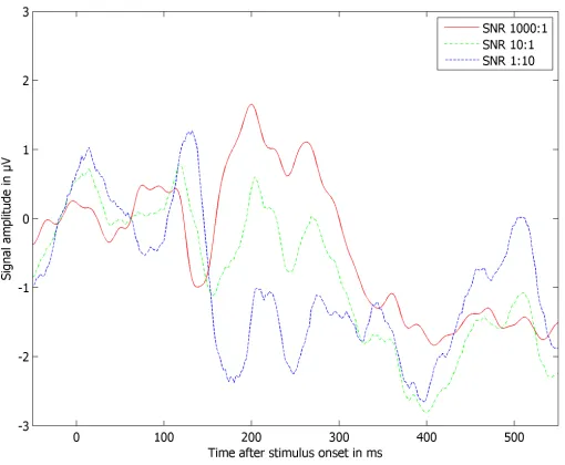
Figure 2. An examplary ERP, contaminated with three variations of the same noise sweep. The noise sweep was scaled by factors of 0.001 (red line), 0.1 (green line), and 10 (blue line). Note that the initially clear peak at 200ms shifts towards 130ms under increasing noise inuence.

4_{In contrast to the original procedure, we used the interior-reective Newton method to solve the}

Simulated trials. The rst analysis used two distinct sample sets. The rst sample set consisted of a grand average ERP of all trials in the dataset. The second sample set contained the 16 subject-specic templates (from the previous section, Templates. Each sample rj(t) from both sample sets was contaminated with 13 levels of noise in two steps:

(a) One noise sweepnj(t)scaled exponentially with a series of factorsνi (iranging between

1 and 13, νi ranging between -3.0 and +3.0). (b) The resulting series of noise sweeps was

then combined with the sample (see gure 2) to create a series of trialsxij(t):

xij(t) =rj(t) + 10νinj(t).

Because noise sweeps were only randomized between trials, not between noise levels, models could produce consistent results across all noise rates.

Methods for P3a estimation

Peak Picking. We used the approach described by Jaskowski and Verleger (2000) verbatim. Both sample and template are examined for the largest positive amplitude. The time dierence between both peaks is dened as estimated P3a latency5_.

Woody's method. We implemented the approach by Jaskowski and Verleger (2000) unaltered. The time oset of the template is varied along the whole timerange, while the covariation between template and sample is calculated. The oset for which the covariation value is maximal was dened as estimated P3a latency.

EML. The implemented method consisted of three parts: the log likelihood function (LLF), the comparison with the noise prole, and the maximum search.

(a) The LLF (Tuan, Möcks, Köhler and Gasser, 1987) estimates which parameter is most likely to describe a given data eld. A frequency component of both sample and template was selected. The two parts were time-shifted across the whole time range and

5_{Note that these methods yield a relative value. To determine the absolute P3a latency in a sample,}

subtracted from each other. The Matlab implementation MLE yielded a log likelihood 6

and a condence interval. Only the log likelihood was used. This operation was conducted for each frequency component, resulting in a likelihood spectrum.

(b) The noise prole (from the previous subchapter, Noise) was divided by the like-lihood spectrum:

X

f

log(Inoise(f))

LLF(sf(t+τj)−rf(t))

Each frequency component was again processed separately. If the time osetτj was perfect,

the signal component would be eliminated from the sample, only leaving noise. This would make the LLF minimal, yielding a maximum result for the formula. For any other time oset

τj, a signal trace remains in the sample, rendering the LLF result larger than minimal.

(c) After establishing the conditions for nding the perfect time oset τj, the goal

was to maximize the division between noise spectrum and LLF result. Including the two variables from before, we had to solve:

maxajmaxτj

X

f

log(Inoise(f))

LLF(ajsf(t+τj)−rf,j(t))

A direct approach was used, varying the values τj and aj one after another. Range and

resolution of τj were straightforward: the length of the whole sample, one datapoint at a

time. The rst step varied only τj, leaving aj at a value of 1. The τj that yielded the

maximum result was considered nal. The factoraj was then varied between 10−1and 101

in 100 linear steps, while searching for a maximum result with the previousτj. The resulting

optimalaj was then used for a third, more accurate search aroundaj±0.1in 39 steps. This

nalaj and the previousτj then dened the estimated P3a latency and amplitude.

Statistics

Two sets of statistics were used to evaluate the validity and performance of the EML, respectively. (a) The three computational models compared samples from two simulated

datasets, against the respective templates. Yielded were the mean squared errors between template-template (expected) and template-sample (estimated) comparisons, as dened by the formula:

M SE= 1

N X

j

(τj−τˆj)2

where τj are the expected and τˆj the estimated latencies. The average MSE over

all subjects was then compared between methods and against the results of the previous study. (b) The EML compared single-trial data from all subjects to a set of subject-specic templates. Results were subjected to bivariate correlation between stimulus intensity and estimated P3a amplitude.

Results

First analysis: Validity of the improved EML

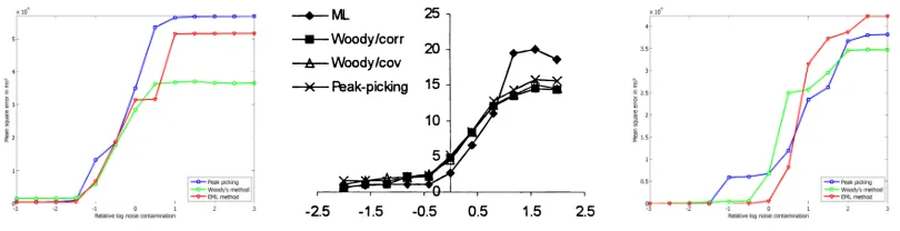
During the rst analysis, accuracy of the three algorithms (peak picking, Woody's method and EML) was compared to the results of Jaskowski and Verleger (2000). Figure 3 (below) displays the eect of noise contamination on the mean squared error of latency estimations. Estimation error from using the articial dataset is displayed in the left-hand chart. Estimation error from using the realistic dataset is presented in the right-hand chart.

The articial condition directly reected on the noise-robustness of the implemented algorithms. Results were accurate in all methods during low-noise conditions. Performance started to degrade at aν of -1.5 (equivalent to a SNR of 30). Error rates increased equally for all three models, until leveling o at ν-values between +0.5 and +1.0. In high-noise conditions, models unanimously detected a P3a-similar complex in the noise sweep. Strong dierences between estimation errors in high-noise conditions mainly result from the low number of random noise sweeps and don't reect on the performance of the algorithm.

The realistic condition was designed to be compared to results from Jaskowski and Verleger (2000). Results were near-perfect in the low-noise region, similar to both the previous condition and the previous study. Degradation started at ν-values between -1.0 and 0.0, which is more diverse than in the previous study (degradation begin at aν of -0.5). Results from peak picking started to degrade rst. Both peak picking and Woody's method started degrading earlier than the EML, but the rate of degradation was lower. Due to this eect, the EML provided the most accurate results up to a ν-value of +0.5. For ν-values of +1.0 and above, the EML yielded the least accurate results for all three models. This result is consistent with the ndings of the previous study: the EML performed best at aν of +0.66 and below, worst at aν of +1.0 and above. In high-noise conditions, peak picking performs slightly worse than Woody's method but better than the EML. Except for the high-noise EML error rate - which was even higher in the previous study - our results are very similar to those of Jaskowski and Verleger (2000).

Second analysis: Connection between pain intensity and detected P3a amplitude

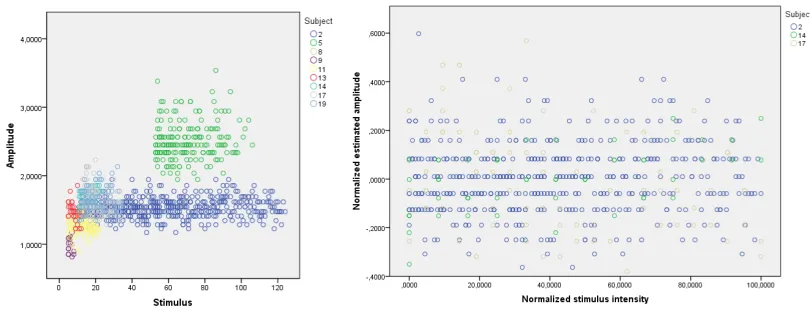
Figure 4. Comparison between stimulus intensity and EML results. Left: Single trials from 9 subjects. Estimated amplitudes are plotted against stimulus intensity. Right: Selection of subjects from the normalized data set; amplitudes are again plotted against stimulus intensity. Note: Appar-ent grouping along the horizontal axis is an artifact from low rounding precision. The correlation analysis is not aected.

The amplitude estimations show large variance between trials. When comparing amplitude estimations against stimulus intensity, no clear pattern or inclination emerges. The bivariate correlation between the two variables doesn't yield signicant results either (r =.038, p(1045) =.225). Post-hoc analysis on a per-subject basis indicates strong

indi-vidual dierences: two subjects reached signicance (r=.208,p(118) =.024; andr=.194,

Discussion

An algorithm was examined for its ability to estimate latency and amplitude in pain-related P3a events. The level of background noise was varied systematically using pseudo-real simulations. The validity of our implementation was conrmed by comparing the results against those of a previous paper. P3a amplitudes were then estimated in a real dataset, failing to detect a connection between stimulus intensity and P3a amplitude.

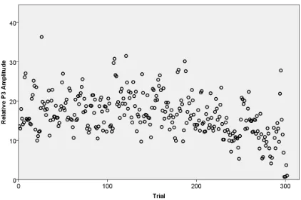
Figure 5. P3a amplitudes from a series of repeated, invariant stimulation. Chart represents stan-dardized and binned data from all subjects.

of 47%).

This nding provides evidence for the third speculation, indicating that EML perfor-mance was limited by the high level of background noise in combination with a low amount of trials.

The vulnerability to low signal-to-noise ratios can be explained by a fundamental limitation of template-based approaches. As ERPs consist of the added eect of a multitude of neuronal clusters, the waveform will inevitably vary strongly between trials - and even more so between subjects. In order to optimize template-based estimations, the template ERP should be as personalized and as noise-free as possible. This poses the rst practical limitation to the application of pain quantication - a large amount of trials is neccessary just to prepare the template and noise prole. Employing a more sophisticated de-noising algorithm (e.g., Quiroga and Garcia, 2003) for each trial could potentially decrease the amount of necessary trials. Another potential remedy to this problem is provided by binning several trials to a less noisy average before employing the amplitude estimation (in our dataset, we reached a 100% detection rate for habituation when combining 4 trials).

specic response that appears to be a single positive peak. If the template approach is desir-able (either in terms of computational eort or robust algorithms), its accuracy potentially could be enhanced by performing a ICA (independent component analysis) which provides localized information to the template. With this compromise, the rigidity problem of the general template is resolved, without having to resort to more complex algorithms. And as the results from the EML estimation have shown, optimization can improve the original algorithm by orders of magnitude - even if the optimization is implemented as nal rene-ment. From this point of view, it would seem benecial to the nal accuracy to vary the components in every possible way - not only amplitude, but also latency, length or even DC oset and frequency baseline.

in P3 detection would combine the positive abilities of all above models (highly adaptive, maximum input granularity, blindly improving process) without many of the drawbacks (templates: rigidity; neuronal networks: scale problems). However, this luxury comes at the cost of very high needs for computational capacity - a common limiting factor in cognitive science.

References

Bromm, B., & Scharein, E. (1982). Principial component analysis of pain-related cerebral poten-tials to mechanical and electrical stimulation in man. Electroencephalography and Clinical Neurophysiology, 53 , 94-103.

Bromm, B., & Treede, R. D. (1991). Laser-evoked cerebral potentials in the assessment of cutaneous pain sensitivity in normal subjects and patients. Revue neurologique, 147 , 625-643.

Coleman, T. F., & Li, Y. (1996). A reective newton method for minimizing a quadratic function subject to bounds on some of the variables. SIAM Journal on Optimization, 6 , 1040-1058. Falkenstein, M., Hohnsbein, J., & Hoormann, J. (1994). Eects of choice complexity on dierent

sub-components of the late positive complex of the event-related potential. Electroencephalography and clinical neurophysiology(2), 148-60.

Gallistel, C. R., Mark, T. A., King, A., & Latham, P. (2002). A test of gibbon's feedforward model of matching. Learning and Motivation, 33 , 46-62. Available from http://bit.ly/af3Djk Houlihan, M. E., McGrath, P. J., Connolly, J. F., Stroink, G., Finley, G. A., Dick, B., et al. (2004).

Assessing the eect of pain on demands for attentional resources using ERPs. International Journal of Psychophysiology, 51 , 181-187.

Jaskowski, P., & Verleger, R. (1999). Amplitudes and latencies of single-trial ERP's estimated by a maximum-likelihood method. IEEE Transactions on Biomedical Engineering, 46 , 987. Jaskowski, P., & Verleger, R. (2000). An evaluation of methods for single-trial estimation of p3

latency. Psychophysiology, 37 , 153-162.

Mahmoodabadi, S. Z., Alirezaie, J., & Babyn, P. (2007). Bio-signal characteristics detection utiliz-ing frequency ordered wavelet packets. In International symposium on signal processutiliz-ing and information technology (p. 748-753).

Polich, J. (2007). Updating p300: an integrative theory of p3a and p3b. Clinical Neurophysiology, 118 , 2128-2148.

Quevedo, A. S., & Coghill, R. C. (2007). Attentional modulation of spatial integration of pain: evidence for dynamic spatial tuning. Journal of Neuroscience, 27 , 11635.

Ranzato, M. A., Huang, F. J., Boureau, Y. L., & LeCun, Y. (2007). Unsupervised learning of invariant feature hierarchies with applications to object recognition. In Computer vision and pattern recognition (p. 1-8).

Smulders, F. T. Y., Kenemans, J. L., & Kok, A. (1994). A comparison of dierent methods for estimating single-trial p300 latencies. Electroencephalography and Clinical Neurophysiology, 92 , 107-114.

Tuan, P. D., Möcks, J., Köhler, W., & Gasser, T. (1987). Variable latencies of noisy signals: estimation and testing in brain potential data. Biometrika, 74 , 525.

Turk, D. C., & Dworkin, R. H. (2004). What should be the core outcomes in chronic pain clinical trials? Arthritis Research and Therapy, 6 , 151-173.