Spike train characterization and decoding for neural prosthetic devices

DEVICES

Thesis by Shiyan Cao

In Partial Fulfillment of the Requirements for the Degree of

Doctor of Philosophy

CALIFORNIA INSTITUTE OF TECHNOLOGY

Pasadena, California 2003

 2003

First and foremost, I would like to express my deepest thanks to my advisor, Professor Joel Burdick, whose keen insight as well as great vision in science and engineering continuously provided me with invaluable advice for the work in this thesis. Undoubtedly, none of the results in this thesis would have materialized without his guidance and support. His encouragement and advising style both on and off the research subject made the last five years truly memorable. I cannot thank him enough for all he has done for me

I owe my special thanks to Professor Richard Andersen, whose knowledge and vision make this research project possible. The collaboration with the Andersen Lab in the past five years was absolutely enjoyable as I was surrounded by talented and devoted scientists and researchers. My special thanks also go to Daniella Meeker, with whom I worked closely on this research project, as her recommendation and data make this thesis possible. In addition I thank Krishna Shenoy, Hans Shoelberg, Zoran Nemadic, Chris Buneo, Aaron Batista…Betty, Kelsie…and many others in the Andersen Lab.

I am also grateful to my friends for their help throughout my ups and downs in the past five years. And finally and most importantly, I want to extend my thanks to my parents for their unconditional support, and to Lap, my wife, for everything she has done for me.

Neural prosthetic device has the potential of benefiting millions of lock-in and spinal cord injury survivors. One branch of the ongoing research is to construct reach movement based prosthetic devices. An important research topic in this area is to accurately and efficiently extract the essential behavioral and cognitive control signals from the relevant brain area, Parietal Reach Region (PRR). This thesis proposes statistical methods based on applying the Haar wavelet packets to spike trains in order to answer some of the questions in this field.

Although spike train is the most frequently used data in the neural science community, its stochastic properties are not fully understood or characterized. Many applications simply assume it is Poisson by nature. This thesis suggests a formal spike train characterization method using the Haar wavelet packet. The Haar wavelet packet projection coefficients are first generated by projecting the observed spike train ensembles onto the Haar wavelet packet function. Then the ensuing empirical distributions of these coefficients are computed. At the same time, the projection coefficients’ distribution of a Poisson process with the same rate function as the observed spike train ensembles are recursively derived. Comparison between the empirical distributions and the hypothesized ones are carried out using a χ2 _{test. If the underlying process of the observed spike trains is indeed Poisson in}

nature, then the two distributions should have good agreement; otherwise, the deviation would be manifested by a large χ2 _{variate. Because of the multi-scale property of the}

wavelet packet, Poisson-ness at different scales can be assessed. Moreover, Poisson Scale-gram is proposed to help visualize the characteristics of the spike train at different scales. Examples from both surrogate and actual data from PRR are subjected to the test.

discriminability is quantified by mutual information, an information theoretic measure. Because of the tree-like hierarchy of the projection coefficients, the extraction method prunes the tree while scoring each feature with mutual information. It returns the most informative feature(s) in the context of the Bayesian classifier. Decoding performance of this proposed method is compared against the one using mean firing rate only on both surrogate data and the actual data from PRR.

It is also crucial to decode cognitive states because they provide the extra control signals necessary for practical implementation of the prosthetic devices. This thesis proposes a simple finite state machine approach where transition occurs among baseline, plan, and go

states. Additionally, an interpreter is introduced to interpret the decoding results and to regulate when the transition should occur. Also, different interpretation rules are explored. This thesis demonstrates that the finite state machine framework, when coupled with the

interpreter, offers a simple autonomous control scheme for the neuron prosthetic system envisioned.

Acknowledgements ...iii

Abstract ...iv

Table of Contents... v

List of Illustrations and/or Tables ...vi

Chapter 1: Introduction... 9

Chapter 2: Background... 18

2.1 Experimental setup and data type ... 18

2.2 Spike train representation... 22

2.3 Haar wavelet packet projection... 24

2.3.1 Haar wavelet review... 24

2.3.2 Haar wavelet packet ... 31

2.3.3 Computing the projection coefficients... 38

2.4 Biologically relevant properties of the Haar wavelet packet ... 39

2.5 Bayesian classifier... 40

Chapter 3: Characterizing spike train processes using Haar wavelet packet... 43

3.1 Introduction ... 43

3.2 Statistics of projection coefficients... 47

3.2.1 Homogeneous Poisson process... 47

3.2.2 Inhomogeneous Poisson process ... 50

3.3 A computational test for Poisson processes ... 53

3.4 Examples... 58

3.5 Conclusion ... 72

Chapter 4: Decoding reach direction using wavelet packet ... 73

4.1 Introduction ... 73

4.2 Feature extraction ... 76

4.2.1 Discriminability and score functions ... 77

4.2.1.1 Mutual information overview ... 78

4.2.1.2 Mutual information and optimal features... 82

4.2.1.3 Estimating mutual information ... 84

4.2.2 Wavelet packet tree pruning ... 85

4.3 Results... 92

4.4 Conclusion ... 107

Chapter 5: Decoding the cognitive control signals for prosthetic systems .... 109

5.1 Introduction ... 109

5.2 Finite state machine modeling of reach movement... 110

5.3 Results... 117

5.4 Conclusion ... 122

Chapter 6: Conclusion ... 123

Bibliography ... 126

Appendix 1... 132

LIST OF FIGURES AND TABLES

Number Page

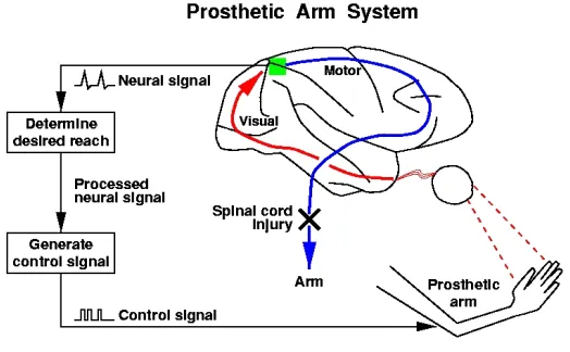
Figure 1-1 Idealized neural prosthetic system ...10

Figure 2-1 Center-out reach task...18

Figure 2-2 Trace of neural activities from a neuron in PRR...20

Figure 2-3 Haar scaling function and Haar wavelet Function on the interval [0 1]....26

Figure 2-4 Haar wavelet and scaling functions up to scale j=2....29

Figure 2-5 Pyramid Algorithm for the special case of Haar wavelet decomposition .31

Figure 2-6 Haar wavelet packet functions up to scale j=2....34

Figure 2-7 Pyramid Algorithm for the Haar wavelet packet decomposition...37

Figure 2-8 Haar wavelet packet function at different scale and locations over 512 units of the basic sampling period δT...40

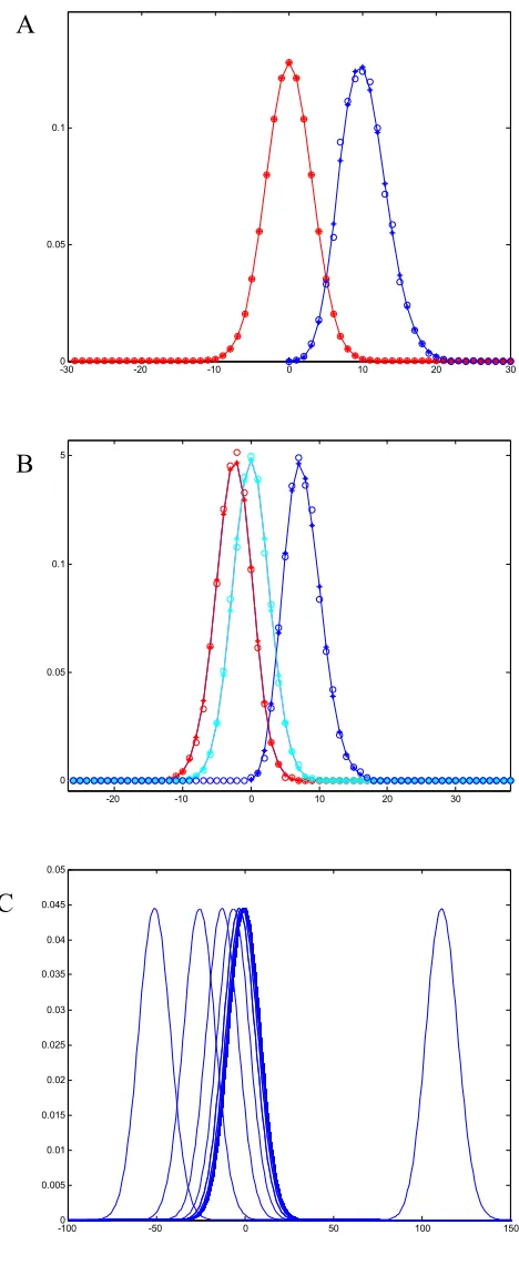
Figure 3-1 Distribution of wavelet packet projection coefficients of Poisson processes61 Figure 3-2 Actual and estimated firing rate function with length T being 512 ms...63

Figure 3-3 Construction of cyclic Poisson spike trains...65

Figure 3-4 Fraction of significantly non-Poisson wavelet packet coefficients, ηj for the 30 neuronal/behavioral combinations from PRR recordings...68

Figure 3.5 Illustration of the Poisson Scale-gram ...69

Figure 3-6. Poisson Scale-grams: Images of the P-values at different scales...70

Figure 4-1 Prune the wavelet packet tree using score function D...91

Figure 4-2 Application of the optimal wavelet packet to the surrogate data...95

Figure 4-3 Application of the optimal selection strategy to the 2nd set of surrogate data98 Figure 4-4 Comparison of mean firing rate and optimal wavelet packet feature for a neuron in binary reach task ...100

Figure 4-5 Binary single neuron reach direction classification performance...102

Figure 4-6 Comparison of mean firing rate and optimal wavelet packet feature for a neuron in 8 direction reach task ...104

Figure 4-7 Comparison of 8-reach direction decoding performance...107

Figure 5-2 Computational architecture for generating high-level, cognitive control signals from PRR pre-movement, plan activity...113 Figure 5-3 Classification time courses, averaged over all reach goal locations, for three different neural population sizes (2, 16 and 41 neurons from monkey DNT) ...119 Figure 5-4 Interpreter performance characteristics...121 Figure A.0-1 Mutual information bounded by the Bayesian classification error E*.

...136 Figure A.0-2 The functionals in Kolmogrov divergence and mutual information

Chapter 1 Introduction

People’s fascination with the brain can be traced back for thousands of years to the time Hippocrates discovered that the brain was involved in sensation and was the source of intelligence. Since then numerous researchers have devoted their careers to unlocking the mystery of the brain: its organization, its functionality, and its operating mechanism. With the advance of physics and electronics in the last century, scientists were able to investigate the brain from its functionality to its microscopic organization. One direct practical result of the explosion of the neuroscience research activities is the development of brain-machine interfaces. Engineers and scientists are using these new scientific discoveries to construct devices that enable the blind to see and the deaf to hear. Another ambitious endeavor is to tap into the thoughts of millions of locked-in patients who are deprived of any motor functions, while their cognitive processing abilities are still functional. With the recent advance of micro-scaled fabrication, probing and recording techniques, reading people’s thoughts has become more than just science fiction.

Neural prosthetic systems are invented under the above premises. They are systems that connect the brain to external devices so that the user can operate the device merely by

Figure 1-1 Idealized neural prosthetic system

In this figure, a patient with spinal cord injury, or lesion, or motor cortex damage is deprived of any limb movement. However, because the functional area in the brain that plans and commands arm-reaching motions is still intact, a neural prosthetic system can extract the thoughts/intentions from this brain area in order to form control signals. Then the signals are relayed directly to a prosthetic arm in order to achieve the desired movement. Visual feedback of the arm’s movement “closes the loop”.

The advantage of using such high-level cognitive brain activities is that they are more anatomically removed from regions that are damaged. While motor areas on the other hand may degenerate following spinal cord injury [Florence 1998, Kaas 2002], most cognitive areas of the brain are known to sustain even after loss of motor functions. Furthermore, the plasticity, which is the capability of learning and adaptation, of the area also holds promise that users may quickly learn to adapt to a brain machine interface [Meeker 2003].

The construction of such a neuro-prosthetic system is no small feat. The quest of designing and building the system involves disciplines ranging from neurobiology to mechanical engineering, in which each field finds its interesting application or challenging questions. Generally speaking, designing and building such a cognitively controlled system requires several large building blocks: behavior experiments and signal harvesting, learning and decoding machinery, control schemes, and system integration. We briefly define each block and its function.

The behavioral experiments are controlled experiments in which the animal performs designated behavior tasks while researchers monitor and record its brain activities. Then either online or off-line, the recorded signals are examined to determine if any possible patterns are embedded in the neural signals so that inferences can be made about the animal’s behavioral states during the experiments. The procedure of inferring the animal’s behaviors or sensory inputs from its recorded brain activities is termed

high-level control schemes necessary for commanding prosthetic devices so that they are directed by the user’s thoughts. Finally, the software and hardware package must be miniaturized for possible clinical implementation.

Among these building blocks, neural decoding is itself a very active research topic. It includes, but is not limited to, characterizing the firing process of the spike trains and estimating or predicting behavioral parameters from neural activities. A topic of ongoing debate in the community is whether spike trains are rate coded or time coded: the former refers to the assumption that the only informative feature in a spike train is the number of spike counts observed in a time window, while the latter refers to the assumption that timing between spike events also plays a role in conveying information. To answer this question, different metrics and approaches ranging from statistical tools to information theory have been proposed over the years [Teich 1986, Holt 1996, Koch 1997, Johnson 1996, Victor 1999, Johnson 2001]. In addition, the quest to promptly and accurately predict some behavioral parameters from neural activities has also attracted large amount of interest, especially in the emerging field of neural prosthetic systems [L. Abbot 1994, Zhang 1997, Schwartz 1988, Moran 1999, Schwartz 2000, Wessberg 2000, Issacs 2000, Nicolelis 2002].

new signal processing technique. Under this approach, the spike trains are projected onto wavelet packets and the distributions of the projection coefficients are analyzed. The coefficients whose empirical distributions significantly deviate from the theoretical distribution of a comparable Poisson process are counted. The higher the counts, the less likely the process is Poisson in nature. It allows us to assess Poisson-ness from different scales, thus avoiding the stationary assumptions employed in some other analysis of the spike trains [Gabbinni and Koch 1998]. Both surrogate data and the spike data collected from neurons in PRR are characterized using this approach.

projection coefficients with the largest decodability towards the decoding task. Finally, I incorporate these selected features into a Bayesian classifier to estimate the behavioral parameters, such as reach directions in the case of decoding from PRR. Again both artificial data and actual neuronal data are used and the decoding performance is compared against the ones using only mean firing rate.

Besides decoding the estimated reach directions from PRR signals, we must estimate additional parameters from neural signals in order to successfully control a robotic device using brain activities. These additional parameters are termed cognitive parameters in this thesis. They describe the brain’s internal behavioral states. For a minimally autonomous robotic device, we define the behavior states to include a baseline state, reach planning states, and the reach execution go state. Because of the structure of the postulated state transitions, we cast them into a novel framework. When combined with an Interpreter that acts on the classification results of these states, it returns an efficient algorithm that extracts the necessary control parameters. Experimental data collected from animals performing a sequence of actions are subjected to this method while we compare different state transition rules.

The contributions of this thesis work include the following:

hand, because of the statistical properties of the Haar wavelet packet, this method provides versatility and insight into the spike train’s characteristics compared to the traditional approaches.

• A wavelet packet based feature extraction method that searches for the most informative features in spike trains is introduced in this thesis. In many decoding problems, researchers automatically use firing rate as the lone feature in their decoding algorithms. Although for spike trains with Poisson nature, firing rate is indeed the only informative feature, as shown in this thesis, not all spike trains exhibit Poisson characteristics. Thus, more generally it is necessary to search for features embedded in the spike trains that are most informative towards decoding. The algorithm introduced here combines information theoretic measures with wavelet packet tree pruning techniques and returns features that offer improved decoding performance.

• Finally, this thesis offers a first look at decoding cognitive states from reach movement sequences. For practical purposes, a neural prosthetic system requires control signals beyond mere reach directions. Thus, this thesis presents a framework based on finite state machine, and different transition rules are explored. Although the framework is very simple, it is the first in the field that demonstrates the feasibility of using cognitive parameters to control autonomous prosthetic arm systems.

• Chapter 2 provides background information on the experimental paradigms used to collect neural data, and introduces the data type used in this thesis. A brief review of the wavelet and wavelet packet concepts, with a focus on Haar wavelet family, is also presented in the chapter. And finally, we review the Bayesian classifier, which is the principal estimation tool used in the thesis.

• Chapter 3 describes a method to characterize spike trains using the Haar wavelet packet function. We investigate the probabilistic properties of the wavelet packet projection coefficients of Poisson processes. From the analysis, we derive both the analytical forms of the distribution and an iterative method that approximate these distributions in practical situations. Additionally this chapter proposes a test that investigates the Poisson-ness of an unknown spike processes. This chapter concludes with applications of the test to different types of data.

• Chapter 5 presents work on decoding logic parameters and sequences of behaviors. We define the necessary states and the state transition concepts that enable a construction of an autonomous model. When coupled with an

Interpreter, this model allows us to integrate decoding with state transition rules so that we can extract practical control signals for a prosthetic system. Several different Interpreter rules are explored as we compare their performance to reach sequences recorded from the animals.

Chapter 2 Background

This chapter provides background information on the experimental setup and the mathematical model of the neural data used in the thesis. Also, brief overviews of wavelet and wavelet packet are presented as well. Finally, we discuss relevant concepts from Bayesian classification, which is the principal classification tool used through out the thesis.

2.1 Experimental setup and data type

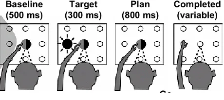
Most of the actual neuronal data used in this thesis are obtained from behavioral experiments that were conducted on Rhesus monkeys (Macaca mulatta) performing delayed center-out reach tasks, which are illustrated in Figure 2.1.

Baseline (500 ms)

Target (300 ms)

Plan (800 ms)

Completed (variable)

Go

Figure 2-1 Center-out reach task

shown target location. A juice reward is administered upon a successful completion of the trial. The target locations are randomly chosen among 8 different locations, and the length of the plan period is also randomized to minimize an anticipation effect [Batista 1999, Meeker 2001].

Alternatively, a virtual reach experiment very similar to the physical reach experiment is carried out in order to simulate a neural prosthesis at work, and also to explore the learning capability of PRR. The distinction between the physical reach and the virtual reach is that in the latter, the animal does not actually perform the reach movement. Instead of moving its arm towards the target, the animal forms the intention of making the movement, which is subsequently decoded. Based on the decoded reach direction, a visual feedback (yellow dot) appears on the touch screen. The animal is given the juice award if the decoded reach direction matches the target.

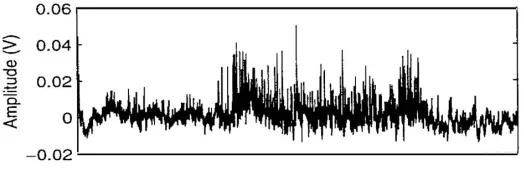
During a recording session, the electrode is first acutely inserted into the brain’s functional area pre-determined using fMRI. Then using a micro-drive, the electrode is advanced incrementally at 700 microns per step in the vicinity of PRR in searching for extra-cellular neuronal activities. Once extra-cellular activities are detected, the animal is required to make a sequence of movements to the 8 different locations in order to decide the relevance of the neuron with respect to the behavior paradigm. If no identifiable correlation exists between the neural activity and the reach locations, the electrode is advanced further until new extra-cellular activities are detected; otherwise, the electrode is fixed at the position that exhibits behaviorally modulated neural activities. Figure 2-2 displays a trace of recorded PRR neural activity. The local surge of the voltage is called the action potential fired by the neuron.

Figure 2-2 Trace of neural activities from a neuron in PRR

X-axis is the time and y-axis is the amplitude in voltage. The sudden surges of the voltage amplitude are action potentials, and the timing of the action potentials marks the occurrence of the spikes.

template method [Lewicki 1998]. Once the spikes are sorted, the time of occurrence of each spike is recorded to a precision of 1ms. A sequence of the spikes forms a spike train, which is one of the most frequently used data types in the neuroscience community. This thesis thus places a strong emphasis on the spike train data format though some of the techniques described have broader applications. The model of the spike train will be the topic of next section.

2.2 Spike train representation

2 ms, the processed and sort signals are down sampled to 1 kHz. This processed version of the spike will be used throughout this thesis.

We employ a standard representation of a spike train as a binary function with 0’s and 1’s. We assume that the onset of a spike can be localized at best to a sampling interval of length δT. Moreover, we assume that spikes are sampled over an interval of length T, where T=2mδT for some integer m. With this assumption, a spike train, s, can be described as Equation 2.1    + = + = = , ] ) 1 ( , [ 0 , ] ) 1 ( , [ 1 ) ( k k k k I in spike no is there if T k T k I in I in spike a is there if T k T k I in t s δ δ δ δ .

Equivalently, a spike train can be interpreted as a T-dimensional vector (where T=2m for some integer m), whose kth element is determined as

Equation 2.2    = + = otherwise T k T k I in spike a exists there if s k k ₀ ] ) 1 ( , [

1 δ δ

,

2.3 Haar Wavelet Packet Projection

We now review the Haar wavelet packet, its waveform, and its construction. Details are outlined in several standard textbooks on wavelet theory [Daubechies 1992, Wickhauser 1994, Mallat 1999, Percival and Walden 2000]. This section also establishes our notation for the projection coefficients of the spike trains. Knowledgeable reader may skip this section and proceed directly to Section 2.4.

2.3.1 Haar Wavelet Review

A wavelet basis is a set of orthonormal functions that partition the time-frequency domain in a dyadic fashion. As shown below, wavelets are constructed from a choice of scaling function and a set of filters. In one sense, a filter can be interpreted as a set of coefficients that are applied to a data stream in order to reveal meaningful features. That is, let a filter be defined by a set of coefficients, {hk}, k=1,..,L. The filter output is given by

∑

=

k

k i k i h x

v ,

We begin with the continuous wavelet function. First we define a low pass filter H by coefficients

{ }

{ }

{ }

{ }

k L k

k h

g =(−1) ₋ , L being the number of filter coefficients. These filters are generally termed Quadrature Mirror Filters (QMF) [Percival 2001]. Next define a scaling function,

) (t

φ , that satisfies the following conditions,

Equation 2.3

∑

∫

∞

∞ − =

= −

= 2 (2 ), ( ) 1

) (

1

dt t k

t h

t L

k

kφ φ

φ .

For simplicity, we denote the analogous operations of convolution and scaling by a factor of two (“decimation”) with respect to the filter pair

{ }

{ }

∑

∑

=

k k k

kf t k Gf g f t k

h

Hf (2 ) (2 ) .

Now construct a function, ψ(t), complimentary to φ(t), such that

Equation 2.4 =

∑

∫

R k

k t k t dt

g

t) 2 (2 ) ( ) 0

( φ ψ

ψ ,

0 0.2 0.4 0.6 0.8 1 0

0.5 1 1.5 2

Haar scaling function

0 0.2 0.4 0.6 0.8 1

-2 -1 0 1 2

Haar wavelet function

Figure 2-3 Haar scaling function and Haar wavelet Function on the interval [0 1].

X-axis is the time in ms and y-axis is the value of the functions.

The strength of wavelet-based analysis for this application resides in both its multi-resolution analysis (MRA) capability and the computational efficiency of the associated numerical algorithms. To understand MRA, consider a nested sequence of subspaces

{ }

integrable functions. These nested subspaces satisfy the following conditions:

C1 _L⊂V_j−1 ⊂V_j ⊂V_j+1 ⊂_L⊂L₂ for all j∈Z, C2 limV_j L₂

j→∞ = ,

C3 lim ={0}

−∞

→ j

j V .

Further, define another complementary set of subspaces

{ }

j j j V W

Combining the above definitions, the spaceL₂(R) can be expressed as

j j W

R

L ∞

−∞ =

⊕ = ) (

2 .

This relation is termed a Multi-Resolution Analysis [Mallat 1999]. Using the actions of translation and dilation, one can construct the following indexed version of the wavelet function, )ψ(t ,

) 2 ( 2 ) ( /2

,k t j jt k

j = ψ −

ψ ,

where j is the scale (or dilation) index and k is the location (or translation) index. Because for a fixed integer j*, the set of functions

{

}

{

}

with different resolutions indexed by j [Percival 2001]. Hence any signal f(t)∈L₂(R) can be represented as a weighted sum of the wavelet bases:

)

(

)

(

t

v

t

f

=

∑

ψ

where the weighting coefficients v_jk are obtained by projection onto the wavelet basis via the regular inner product on L₂(R),

dt

t

t

f

v

=

∫

(

)

ψ

(

)

Even though the MRA is defined for the continuous function space, L₂(R), its construction can be easily generalized to the domain of discrete data. Consider a vector X

sampling interval of the discrete data. We denote the resulting set of adapted scaling functions as φ_0k(t), whose support is

[

]

{ }

{ }

Equation 2.5 =

∑

l l k l k h 2 0

1 φ

φ ,

Equation 2.6 =

∑

l l k l k g 2 0

1 φ

ψ .

We note the support of the functions φ_1k(t) and ψ_1k(t) is

[

]

1 2 ,...,

0 −

= T

k . Moreover, the sets of functions φ_1k(t) and ψ_1k(t) are called the scaling

function and the wavelet functions at scale j=1. We can extend Equation 2.3 and Equation 2.4 recursively for all j such that

Equation 2.7 =

∑

l

l j k l jk h 2 φ 1

φ ,

Equation 2.8 =

∑

l l k j l jk g 2 φ 1

ψ ,

where the sets of functions φ_jk(t) and ψ_jk(t) are called the scaling function and the wavelet functions at scale j, and their support is

[

]

stops at scale j=log2T, where both the wavelet function and the scaling function have

support [0 T], with T being the presumed length of the spike train data sequence. For the Haar wavelet function, the low pass filter and the high pass filter are {h0=1 h1=1} and

{g0=-1 g1=1 } respectively. The scaling and wavelet function up to scale j=2 are plotted

0 2 4 0 0.2 0.4 0.6 0.8 1 1.2

0 2 4

0 0.2 0.4 0.6 0.8 1 1.2

0 2 4

0 0.2 0.4 0.6 0.8 1 1.2

0 2 4

0 0.2 0.4 0.6 0.8 1 1.2

0 1 2 3 4

-1 -0.5 0 0.5 1

0 1 2 3 4

-1 -0.5 0 0.5 1

0 1 2 3 4

-1 -0.5 0 0.5 1

0 1 2 3 4

-1 -0.5 0 0.5 1

0 1 2 3 4

-1 -0.5 0 0.5 1

0 1 2 3 4

-1 -0.5 0 0.5 1

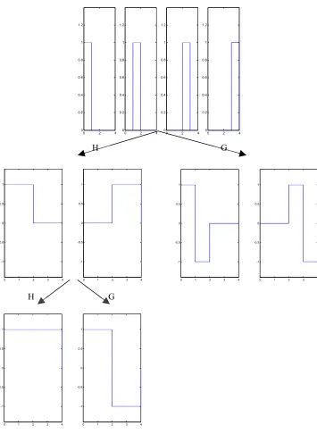
Figure 2-4 Haar wavelet and scaling functions up to scale j=2.

The top panel contains the scaling functions at scale j=0, for this example, k=1,2,3,4. The middle left panel contains the scaling function at scale j=1, and the middle right panel contains the wavelet function at scale j=1. The bottom left panel is the scaling function at scale j=2, and the bottom right panel is the wavelet function at scale j=2. The symbols H and G indicate the filtering operation that

generates these functions. Notice the support at each scale increases dyadicly.

This recursive relationship also enables MRA in the discrete context.

H

H G

The above application of the wavelet functions to the discrete data inspires the so-called

Pyramid Algorithm [Mallat 1999], an efficient method for computing the wavelet

projection coefficients of discrete data. Again we take a vector X={x0,…,xT-1} in RT, the

space of all T-dimensional vectors, where T is a power of 2. Similarly, we interpret the vector X as a piece-wise constant continuous function with constant values xk over the

sampling interval

[

]

∫

= X t t dt u_0k ( )φ_0k( ) .

Because X(t) is a piece-wise constant function with piecewise support coinciding with the support of φ_0k(t), and by Equation 2.3,

k k x

u₀ = .

Therefore, the finest scale coefficients are exactly the input data itself. Now we can use the low pass filter

{ }

{ }

Equation 2.9 =

∑

l l k j l jk h u

u _{2 1,} ,

Equation 2.10 =

∑

l

l j k l jk g u

v _{2 1,} ,

where the {vjk} are the wavelet projection coefficients and the {ujk} are the scaling

and {ujk} at each scale are T_j

2 . For the Haar wavelet, we can illustrate the idea behind the Pyramid algorithm using a decomposition tree similar to the one illustrated in Figure 2.4, where each node at level j in the tree represents a set of wavelet coefficients at scale level j (Figure 2.5).

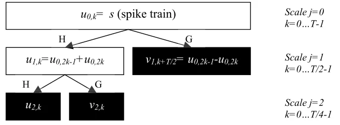
Figure 2-5 Pyramid Algorithm for the special case of Haar wavelet decomposition

At scale j=0, the scaling coefficients u0,k are the input data sequence whose length is T. At scale j = 1,

we obtain the scaling coefficients u1,k and wavelet coefficients v1,k by performing the convolution-decimation operation with H and G, respectively. Note the cardinality of the coefficient set is now T/2

because of the decimation. The two nodes at j=1 are termed children of the parent node at j=0

because they are derived from that parent node. Similarly, the scaling coefficients u2,k and wavelet coefficients v2,k at scale j=2 are generated from the parent node at scale j=1, and their corresponding

cardinality is T/4. Using this algorithm, we can proceed to calculate the wavelet coefficients at all scales until the size of the coefficient set equals 1.

2.3.2 Haar Wavelet Packet

The wavelet packet is an extension of the basic wavelet construction described above. Because wavelet packets are a super-set of wavelets, they offer a richer selection of basis functions. In the context of the spike train classification problem, this added richness yields a more refined analysis of the spike train. The construction of the continuous Haar wavelet packet basis functions again involves a low pass filter

{ } { }

{ } { }

u0,k= s (spike train)

u1,k=u0,2k-1+u0,2k v1,k+T/2= u0,2k-1-u0,2k

u2,k v2,k

H

H

G

G

Scale j=0 k=0…T-1

Scale j=1 k=0…T/2-1

defined below have support on the real interval [0 1], we can again apply the convolution and decimation operation recursively to define the set of functions,

∑

∑

k k n n k n k n k t g t k t h t ) 2 ( ) ( ) 2 ( ) ( 1 2 2 ψ ψ ψ ψ ,

where the sum is over the cardinality of the filter coefficients hk and gk, and for the Haar

wavelet,

[

)

Note that ψ0is the same as the Haar wavelet scaling function, and ψ1 is the Haar wavelet

described above.

Like wavelets, wavelet packets can be extended to the discrete MRA using the double index of scale j and location k. Consider a vector X in RT, the space of all T-dimensional vectors, where T is again a power of 2. With the interpretation of the piece-wise constant function in Section 2.3.1, the scaling function φ(t) is first scaled and adapted to each sampling interval of the discrete data. We denote the resulting set of adapted scaling functions as ψ_0k(t), where

Equation 2.11

[

]

   ∈ + = otherwise T k T k t if t k ₀ ) 1 ( , 1 ) ( 0 δ δ ψ ,

whose support is

[

]

{ }

and the high pass filter

{ }

Equation 2.12 =

∑

l

Equation 2.13

∑

jk _j g 2 1

2

ψ

ψ ,

where the sets of functions ψ_jk(t) have support

[

]

summation is the cardinality of the filter coefficients H and G. The recursion stops at scale j=log2T, where both the wavelet packet functions have support [0 T]. For the Haar

wavelet function, the low pass filter and the high pass filter are {h0=1 h1=1} and {g0=-1

g1=1 } respectively, thus the relationship becomes

) ( )

( )

( _{1,2 1 1,2}

,k t j k t j k t

j =ψ − − +ψ −

ψ , if low pass

) ( )

( )

( _{1,2 1 1,2}

2

,k T t j k t j k t

j + _j =ψ − − −ψ −

ψ , if high pass

where j is the scale index, k is the position index, and T is the length of support of the filter at the largest scale, as defined above. An example of Haar wavelet packets and their recursion relationship is shown graphically in Figure 2-6.

0 2 4

0 0.2 0.4 0.6 0.8 1 1.2

0 2 4

0 0.2 0.4 0.6 0.8 1 1.2

0 2 4

0 0.2 0.4 0.6 0.8 1 1.2

0 2 4

0 0.2 0.4 0.6 0.8 1 1.2

H G

0 1 2 3 4 -1 -0.5 0 0.5 1

0 1 2 3 4

-1 -0.5 0 0.5 1

0 1 2 3 4

-1 -0.5 0 0.5 1

0 1 2 3 4

-1 -0.5 0 0.5 1

0 1 2 3 4

-1 -0.5 0 0.5 1

0 1 2 3 4

-1 -0.5 0 0.5 1

0 1 2 3 4

-1 -0.5 0 0.5 1

0 1 2 3 4

-1 -0.5 0 0.5 1

0 0.5 1

0 0.5 1 1.5

0 0.5 1

-2 0 2

0 0.5 1

-2 0 2

Haar Wavelet Packet--indexed at 19

0 0.5 1

-2 0 2

0 0.5 1

-2 0 2

0 0.5 1

-2 0 2

0 0.5 1

-2 0 2

0 0.5 1

-2 0 2

0 0.5 1

-2 0 2

0 0.5 1

-2 0 2

0 0.5 1

-2 0 2

0 0.5 1

-2 0 2

0 0.5 1

-2 0 2

0 0.5 1

-2 0 2

0 0.5 1

-2 0 2

0 0.5 1

-2 0 2

0 0.5 1

-2 0 2

0 0.5 1

-2 0 2

0 0.5 1

-2 0 2

0 0.5 1

-2 0 2

Figure 2-6 Haar wavelet packet functions up to scale j=2.

H G H G

A) The top panel contains the wavelet packet functions at scale j=0. It is identical to the scaling function. The middle left panels contain the wavelet packet functions at scale j=1 as a results of the

low pass filtering, and the middle right panels contain ones as a results of high pass filtering. The two bottom left panels contain the wavelet packet functions that are children of the two middle left ones, and similarly the two bottom right ones are children of the two middle right ones. The H and G

indicate the filtering operation towards these functions. Notice the support at each scale increases dyadicly. B) The Haar wavelet packet functions on [0 1] up to the 19th _iteration.

In particular, we notice that the set of Haar wavelet functions is the left vertical branch in the packet tree (Figure 2.6A).

An interesting property of the Haar wavelet packet functions is the orthogonal relationship between all of the packet functions. Before describing the orthogonality in detail, we first define several relevant terms. A tree is an arrangement of the wavelet packet functions such that they are structured in a branching fashion. A nodeN_jl is either a tree branches or a tree leaf, and at a given scale j there are 2j nodes. In the above example, there are 1 node N01 at scale j=0, 2 nodes at scale j=2, and 4 nodes at scale j=3.

Moreover, the member functions of a node are defined as the wavelet packet functions related to each node. The relationship is the constructive iteration shown in Figure 2.6. The number of member functions for any node at scale j is T/2j, where T is the length of the input vector under investigation. Now we are in position to discuss the orthogonality property.

Proposition 2.1 Member functions of each node are orthogonal to the member functions

For example, in the above figure, the member functions of N21 are orthogonal to the

members of N22, N23, and N24. Likewise, it is also orthogonal to the parent node of N23

and N24, namely N12 because N21 and N12 do not share a branch.

Proof:

Note that the member functions of any two child nodes derived from the same parent are orthogonal. To show this, directly integrate the functions:

∫

where )(

1 t

jk

ψ is a member function of

1

jl

N and )(

2 t

jk

ψ is a member function of

2

jl

N .

There are two possibilities for the above integration:

1) If k₂ ≠k₁₊₂J−j, then

∫

non-overlapping support. 2) If k₂ =k₁₊₂J−j, then

0 ) ( ) ( )] ( ) ( )][ ( ) ( [ ) ( ) ( 2 2 , 1 2 1 2 , 1 2 , 1 1 2 , 1 2 , 1 1 2 , 1 1 1 1 1 1 1 2 1 = − = − + = − − − − − − − − −

∫

∫

∫

In addition, the wavelet packet functions contained in the branches derived from the two child nodes are also orthogonal. To see this, we observe that the space spanned by the first child node is orthogonal to the one spanned by the second child, i.e.,

{ }

1 Span jk

S = ψ , k₁∈child node 1

{ }

2 Span jk

2

1 S

S ⊥

because the member functions,

{ }

1

jk

ψ and

{ }

2

jk

ψ are orthogonal as shown earlier. Moreover, the wavelet packets contained in the branches of the two child nodes are linear combinations of the ones in

{ }

{ }

Therefore, we have shown that the wavelet packet functions in any node are orthogonal to the ones in nodes that are a member of a different branch. ٱ

Similarly, we can adopt the Pyramid Algorithm to efficiently compute the projection coefficients of the wavelet packets. The algorithm is almost identical to the one used for wavelets, with the only difference being that the branching of the wavelet packet tree occurs at every node, while branching occurs only in the first node of its wavelet counterpart. We can likewise devise a tree diagram to illustrate the decomposition of a T -dimensional vector (Figure 2-7)

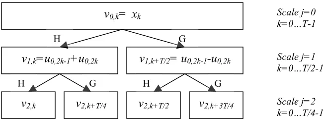
Figure 2-7 Pyramid Algorithm for the Haar wavelet packet decomposition

At scale j=0, the coefficients v0,k are the input data sequence whose length is T. At scale j = 1, we

obtain the coefficients v1,k and v1,k+T/2 by performing the convolution-decimation operation with H and G, respectively. Note the cardinality of the coefficient set is now T/2 because of the decimation.

The two nodes at j=1 are termed children of the parent node at j=0 because they are derived from v0,k= xk

v1,k=u0,2k-1+u0,2k v1,k+T/2= u0,2k-1-u0,2k

v2,k v2,k+T/4

H

H

G

G

Scale j=0 k=0…T-1

Scale j=1 k=0…T/2-1

Scale j=2 k=0…T/4-1 v2,k+T/2 v2,k+3T/4

that parent node. Similarly, the same relationship is observed at scale j=2, in which the cardinality of the coefficients in each node becomes T/4.

Using this version of the Pyramid Algorithm, we can efficiently compute all the wavelet packet coefficients up to scale j=log2T. In all, the wavelet packet decomposition of a

vector of length T returns TlogT wavelet packet coefficients, compared to the T

coefficients by wavelet decomposition.

2.3.3 Computing the Projection Coefficients

Using the concepts and the background presented in the previous sections, the T -dimensional spike train, s={s0,…,sT-1} can be projected onto the Haar wavelet packets

using the aforementioned Pyramid Algorithm.

Based on spike train model shown in Section 1, the 0th scale wavelet packet coefficients

v0,k are precisely the original spike train sk,

Equation 2.14 v0k =sk.

For the Haar wavelet packet, the recursive relations for the remaining coefficients then become

) ( )

( )

( _{1,2 1 1,2}

, t v t v t

v_jk = _{j− k−} + _{j− k} , if low pass )

( )

( )

( _{1,2 1 1,2}

2

, t v t v t

v _{T j k j k}

k

2.4 Biologically Relevant Properties of the Haar Wavelet

Packet

Although there are many possible choices of wavelet functions, the Haar wavelet packet carries some special properties which make it an appealing choice for projecting, analyzing, and interpreting spike trains. As seen in Section 2.3, the Haar wavelet packet functions have compact support in the time domain. This bodes well with the fact that spike trains consist of spike signals with support as small as the sampling interval δT. In other words, Haar wavelet packet functions completely capture the discrete nature of the spike trains. On the other hand, other basis functions such as trigonometric functions would produce undesirable artifacts because of Gibb’s phenomenon. Furthermore, some of the Haar wavelet packet projection coefficients have intuitive interpretations that relate them to measures widely recognized in neuroscience. For example, the coefficient vj1 at

a scale j corresponds to the number of spikes in a window of length _T/2j_{, with which}

we can express the mean firing rate in that window as ₂jv_{j /}T

1 . In other words, the vj1

corresponds to the mean firing rate in an associated time interval, or window (see Figure 2-8a). Furthermore, coefficients such as vj2 are closely tied to the local change of firing

0 50 100 150 200 250 300 350 400 450 500 -2

-1 0 1 2

A

0 50 100 150 200 250 300 350 400 450 500

-2 -1 0 1 2

B

0 50 100 150 200 250 300 350 400 450 500

-2 -1 0 1 2

C

Figure 2-8 Haar wavelet packet function at different scale and locations over 512 units of the basic sampling period δT

A. j=9, k=1, the wavelet packet function corresponds to a window that spans the whole 512 units. Consequentially, the resulting coefficient v9,1 correlates to the mean firing rate in the sampling window of length 512 δT. B. j=6, k = 10, the wavelet packet function corresponds to one up-down cycle over 64 units. The resulting coefficient v6,10 in this case represents the difference of the firing rate in two consecutive 32 units windows. C. j = 4, k =300, the wavelet packet function corresponds to high frequency oscillation in a 16 units window. The resulting wavelet coefficients v4,300 have direct

implication on local bursting activities.

2.5 Bayesian

classifier

This section reviews basic concepts about the Bayesian classifier, a widely used classification method. It classifies an unlabeled observation by estimating its probability associated with each different class. More rigorously, denote the stimulus parameter (class label) as X and the feature (unlabeled observation) as v, both are random variables. Then the ubiquitous Bayes’ rule states that

Equation 2.15

) (

) ( ) | ( ) | (

v P

X P X v P v X

where X is the class label, v is the feature, P(X|v) is the posterior probability, P(X) is the prior probability of X, and P(v|X) is the likelihood of v given X. In this thesis X is interpreted as the reach direction, and v as the neural signals. Bayesian classification is based on the principle,

Equation 2.16 argmax

{

}

~

v X P X

X

= ,

the estimated class or reach direction X~ is the one that maximizes the posterior probability P(X|v).

Since the conditional probability p(v|X) must be estimated, this thesis estimates the conditional densities using the Parzen window method [Parzen 1965]. The Parzen window approach applies Gaussian kernels to the observed data and returns density estimation in the form of the normalized sum of Gaussians centered at each data point. We can write the resulting density function as

∑

− =

= Nc

i i

c

v v G N c X v p

1

) , ( 1

) |

( σ ,

where G(v, σ) is a Gaussian kernel with standard deviation σ, and Nc is the total number

of trials in class Xc. Clearly p(v|X=c) is a density function because it integrates to 1 over

A special case of the classification problems is the binary classification problem. Because of its simplicity, many well-established theories of pattern recognition are built upon the binary classification problem. Let the two classes be X1=1 and X2=0. The

Bayesian classification rule can be defined as

Equation 2.17

 

 = >

=

otherwise v X P if x

g

0

2 / 1 ) | 1 ( 1

) (

* _.

Interestingly this simple classification rule turns out be the optimal binary classifier. Define the classification error E as

Equation 2.18

) ( ) | ~ (

) ~ (

v P v X X P

X X P E

v

∑

=

≠ =

.

Theorem 2.1: [Devroye 1998] Let the Bayesian classification error be E*. That is, E* is

the error in the estimate produced by Equation 2.16, then E* ≤E_{for all E.}

Chapter 3 Characterizing spike train processes using

Haar wavelet packet

3.1 Introduction

A sequence of spikes forms a spike train, which is often modeled as a random process [F. Rieke 1997]. It is the most widely used data type in the neuroscience community. Problems, such as neural encoding and decoding given spikes, have been studied extensively [Gabbiani and Koch 1998, Rieke 1997, Victor 1997, Strong 1998, Johnson 1996, 2001]. However, the precise characteristics of this random process are still an open question. Researchers have proposed different models to capture the statistical characteristics of spike trains while the debate over the correctness of rate coding or temporal coding of spike trains has been on going for some years [Johnson 1996, 2001, Reich 2000, Steveninck, 2002]. Here rate coding refers to the assumption that information is only conveyed in the firing rate of the spike train, and time coding refers to the assumption that precise timing of the spikes also codes information. Schemes that better characterize the firing process will help to understand the underlying neural code.

( )

n T n

p = λ −λ

! )

( .

Thus, for a homogeneous Poisson process the mean and variance of the spike counts up to time T are both λT. The ratio of the variance to the mean is termed the Fano factor. A unit value of this factor can indicate the presence of a Poisson process [Rieke 1997]. However, the Fano factor only focuses on the first two moments of a spike train’s statistical characterization, while discarding the remaining higher ones. One can also measure the coefficient of variation (COV), which is the ratio of the standard deviation to the mean of the inter-spike intervals [Gabbiani and Koch 1998]. In the case of a Poisson process, the COV is 1, which exemplifies one of the properties of a Poisson process: the inter-spike intervals are exponentially distributed. However, using the COV as a measure discards the possibility of discovering any possible patterns embedded in the spike trains [Gabbiani and Koch 1998]. Another approach is to project the auto-correlation function of a spike train onto a Fourier basis, and examine the resulting power spectral function [Gabbiani and Koch 1998]. For a Poisson process, the power spectrum should be flat everywhere except at the origin. Yet, the use of the auto-correlation function assumes by default that the underlying spike generation process is stationary. When this assumption is violated, blindly applying the power spectrum may produce artifacts in the frequency domain [Mallat 1999]. The method described in this chapter can be applied to mildly nonstationary signals.

coefficients obtained by projecting ensembles of the spike trains onto the wavelet packets are random variables themselves. The statistical properties of the projection coefficients shed light on the statistical nature of the spike train. This thesis shows that the distribution of the projection coefficients for both homogeneous and inhomogeneous Poisson processes can be well characterized. Using hypothesis testing on the coefficient statistics, one can determine if a spike train is well characterized as a homogeneous or inhomogeneous Poisson process. If the spike train is not deemed to be a Poisson process, then this method also suggests the degree of non-Poisson-ness, and also highlights the spike train’s characteristic time scales at which the spike train exhibits non-Poisson behavior. To help visualize the degree of non-Poissonness at different scale, the Poisson scale-gram is introduced. Taken together, these analyses provide guidance for further investigations of a neural process in the case that it is significantly non-Poisson.

Generally, wavelet-based analysis is more suitable than Fourier analysis when dealing with non-stationarity and specifically locally stationary processes [Mallat, 1998]. Power spectrum based characterization method often encounters Gibbs phenomenon in which local discontinuity of the signal produces bleeding of power into the higher frequency domain, thus creating artifacts in the spectral-gram [Mallat 1999]. By using wavelet-based methods, the spike train characterization technique presented here overcomes some of the disadvantages of the methods reviewed above. Moreover, the multi-resolution analysis feature of wavelets provides additional versatility in handling possible patterns embedded in the spike trains. In this chapter, a wavelet basis consisting of the Haar wavelet packet, which is an extension of the Haar wavelet [Wickerhauser 1994, Mallat 1999, Percival and Walden 2000], is the basis of the computational test. Some of the Haar wavelet packet’s special properties, such as compactness and biologically intuitive interpretations of the projection coefficients (see Section 2.2), make it an ideal candidate for decomposing spike trains. Note that others have explored the possibility of using wavelet packets as a mean of processing spike data [Kralik 2001, Oweiss 2001, 2002]. Yet, the work in this thesis appears to be the first to use wavelet methods for formal characterization of spike trains.

in Section 4 we integrate these ideas into a methodology that characterizes spike train modeled as stochastic point processes. Several examples illustrate the main points in Section 5.

3.2 Statistics of projection coefficients

Chapter 2 reviewed the concepts underlying the construction of Haar wavelet packets, and introduced the projection coefficients arising from a binary spike train. This section investigates the statistics of these coefficients when the given firing process is a homogeneous or inhomogeneous Poisson process. Using a hypothesis testing methodology based on a χ2_{-statistic applied to the coefficient distributions, one can then}

check if a given spike train is statistically close to a Poisson process by comparing the statistics of the projected data against the formulas derived below. This hypothesis testing approach is developed in the next section.

3.2.1 Homogeneous Poisson Process

For simplicity, let us first analyze the case of a homogeneous Poisson process with a constant firing rate λ. Poisson processes have three relevant properties:

P1. Each non-overlapping time increment of a Poisson process is independent and identically distributed with the probability, P(.) of a spike occurring in the interval [t,t+∆t] given by

t N

N

P( _t+∆t − _t =1)≈λ∆ ,

P2. When conditioned on a fixed number of spikes, a Poisson process uniformly distributes all the spikes in a window of length T. We can formulate this mathematically as

T t N

t t t t

P( '< < '+∆ | =1)= ∆ ,

i.e. given that only 1 spike occurs somewhere in a window of length T, the probability of observing that spike in a any interval of length ∆t is

T t

∆ .

P3. The probability of observing n spikes in a window of length T given the firing rate

λ is

( )

n T n

P = λ −λ

! )

( .

Now we derive the probability distributions of wavelet packet coefficients generated by the projection of an ensemble of spike trains that arises from a homogeneous Poisson process with fixed firing rate λ onto the Haar wavelet packet. First, notice that the resulting projection coefficients are integer valued because the Haar wavelet packets are functions that assume the value -1 and 1 only; and the spike trains are similarly binary valued. Also, recall from Equation 2.2 that the integrals of wavelet packet functions at all scales are 0. This symmetry of the wavelet packet, when coupled with property P2, implies that when a single spike is projected onto the support of a wavelet packet function, the probabilities of the resulting coefficient being 1 or -1 are the same, namely ½. Based on this observation, we can write the conditional probabilities of the projection coefficients as follows: given N spikes in a window of length T,

            = −

=

n N N

n N v P

N

2 1 ) | 2

where )P(v=k|N is the probability that coefficient v takes the integer value k when N

spikes occur in the support of the wavelet packet function associated with coefficient ν. In addition, we can write

∑

∑

P( ) ( , ) ( | ) ( ),

where P(N) is the probability of finding N spikes in the time interval of length T, expressed by property P3. Thus, the probability of observing a projection coefficient of integer value n is

Equation 3.1 T

N N N e N T n N N n v

P ∞ λ −λ

=

∑

, if n is even

Equation 3.2 T

N N N e N T n N N n v

P ∞ λ −λ

=

∑

, if n is odd.

in the interval∆t₁ with probability ½, then the second spike has to reside in ∆t₂ with probability 1. Therefore, we see that the approximation breaks down in this case. In the next section, where the more general case of inhomogeneous Poisson processes are considered, I propose a computational approach that approximates those probabilities so that they are not susceptible to discretization errors. In addition, the computational approach can be generalized to inhomogeneous Poisson processes. The theoretical derivations of this section provide a standard against which we can check our computational theory in the simple case of a purely homogeneous Poisson process.

3.2.2 Inhomogeneous Poisson Process

An inhomogeneous Poisson process is a Poisson process with a variable firing rate λ(t). Even though it’s not stationary like a homogeneous Poisson process, it retains the same memoryless property, P2, namely that disjoint increments of an inhomogeneous Poisson process are independent.

Due to the variable firing rate, the approach outlined in the previous section becomes unfeasible for inhomogeneous Poisson processes because the probability of observing n

spikes in an interval of duration T is now a combinatorial problem that depends on the cardinality of the different firing rates present in this interval. Fortunately, a simpler alternative to the computation of the coefficient distributions exists by utilizing the Pyramid Algorithm and the memory-less property of an inhomogeneous Poisson process. Recall that an inhomogeneous Poisson process has independent disjoint increments, i.e.,

) ( ) ( ) ,

(v_0,k v_0,k+1 =P v_0,k P v_0,k+1

where,

Equation 3.3 P(v _k =0)=e−λk∆T

, 0

Equation 3.4 P(v _k =1)≈1−e−λk∆T

,

0 ,

where that v0,k is the 0th level wavelet packet projection of the point process at location k.

It is a random variable indicating whether a spike is present in the kth time increment. Equation 3.3 is the direct result of property P3, while Equation 3.4 is a reasonable approximation when the time interval ∆T is small. Also recall that the Pyramid Algorithm for the Haar wavelet consists of a low-pass filter

{ }

{ }

k k T k k k k v v v v v v 2 , 0 1 2 , 0 2 , 1 2 , 0 1 2 , 0 , 1 − = + = − + − , for 2 ,..., 2 , 1 T

k = .

The following proposition illustrates the independence of these wavelet packet coefficients.

Proposition 3.1: For a given homogeneous or inhomogeneous Poisson process,

the wavelet packet coefficients contained in any node of the wavelet packet tree, namely

{ }

T l

lT k jk

v ( 1) /2 2 / 1 +

+

= , 1=0,1,...,2 −

j

l , are independent.

{ }

T l

lT k jk

v ( 1) /2 2 / 1 + +

= is the set of

the length of the spike train in multiples of δt. And l indexes the nodes at a particular scale.

The proof of this proposition can be found in Appendix 1.

Based on the structural independence established by Proposition 3.1, the respective probabilities of the coefficients v1,j then become

Equation 3.5 = =

∑

−

n

v

k v P n P v n

v P

k k

v ( ) ( )

) (

2 , 0 1 2 , 0 ,

1 if k≤T/2

Equation 3.6 = =

∑

−

n

v

k v P n P v n

v

P _k