ENERGETIC VARIATIONAL APPROACH IN COMPLEX FLUIDS:
MAXIMUM DISSIPATION PRINCIPLE
By
Yunkyong Hyon
Do Young Kwak
and
Chun Liu
IMA Preprint Series # 2228
( November 2008 )
INSTITUTE FOR MATHEMATICS AND ITS APPLICATIONS
UNIVERSITY OF MINNESOTA
400 Lind Hall
207 Church Street S.E.
Minneapolis, Minnesota 55455–0436
ENERGETIC VARIATIONAL APPROACH IN COMPLEX FLUIDS :
MAXIMUM DISSIPATION PRINCIPLE∗
Y. HYON †, D. Y. KWAK‡, AND C. LIU§
Abstract. We discuss the general energetic variational approaches for hydrodynamic systems of complex fluids. In these energetic variational approaches, the least action principle (LAP) with action functional gives the Hamiltonian parts (conservative force) of the hydrodynamic systems, and the maximum/minimum dissipation principle (MDP), i.e., Onsager’s principle, gives the dissipative parts (dissipative force) of the systems. When we combine the two systems derived from the two different principles, we obtain a whole coupled nonlinear system of equations satisfying the dissipative energy laws. We will discuss the important roles of MDP in designing numerical method for computations of hydrodynamic system in complex fluids. We will reformulate the dissipation in energy equation in terms of a rate in time by using an appropriate evolution equations, then the MDP is employed in the reformulated dissipation to obtain the dissipative force for the hydrodynamic system. The systems are consistent with the Hamiltonian parts which are derived from LAP. This procedure allows the usage of lower order element (a continuousC0
finite element) in numerical method to solve the system rather than high order elements, and at the same time preserves the dissipative energy law. We also verify this method through some numerical experiments in simulating the free interface motion in the mixture of two different fluids.
Key words. Energetic variational approach, dissipation energy law, least action principle, maximum dissipation principle, Navier-Stokes equation, phase field equations.
AMS subject classifications. 76A05, 76M99, 65C30
1. Introduction. The energetic variational approaches of hydrodynamic
sys-tems in complex fluids are the direct consequence of the second law of thermodynam-ics. The complex fluids in our interests are the fluids with micro-structures (molecular configurations), for instance, viscoelastic polymer models such as Hookean model, fi-nite extensible nonlinear elastic (FENE) dumbbell models, rod like liquid crystal mod-els, and multi-phase fluids [1, 2, 3, 7, 8, 14, 19, 25, 31, 32]. The interaction/coupling between different scales or phases, plays a crucial role in understanding complex fluids. The interaction in polymeric fluids [2, 3, 8, 14, 25] can be described by the macro-scopic deformation to the micromacro-scopic structure through kinematic transport and the macroscopic elastic stresses induced by the molecular configurations in microscopic level. A competition in multi-phase fluids [1, 19, 31, 32] can be described by the macroscopic kinetic energy and the internal “elastic” energy through the kinematic transport. The complex fluids thus are basically described by multiscale-multiphysics model.
We illustrate the energetic variational approach for one of complex fluid model using the least action principle (LAP) [15] and the maximum/minimum dissipation principle (MDP) [22, 23, 24] to understand complex fluids. In computational view-point the MDP shows a way to achieve an efficient method for numerical computations.
∗THE WORK OF LIU AND HYON IS PARTIALLY SUPPORTED BY THE NSF GRANTS
NSF-DMS 0707594. THE WORK OF KWAK IS SUPPORTED BY KOSEF GRANT BY KOREA GOVERNMENT R01-2007-000-10062-0
†Institute for Mathematics and Its Applications, 114 Lind, 207 Church St. S.E., Minneapolis,
MN 55455, USA, email:[email protected],
‡Department of Mathematical Science, Korea Advanced Institute of Science and Technology,
Korea, email: [email protected]
§Department of Mathematics, Pennsylvania State University, University Park, PA 16802, USA,
The energetic variation is based on the following energy dissipation law for the whole coupled system:
dEtotal
dt =−△
where Etotal is the total energy of system and△is the dissipation [22, 23, 24]. The
LAP, which is also referred as the Hamiltonian principle, or principle of virtual work, gives us the Hamiltonian (reversible) part of the system related to the conservative force. At the same time, the MDP gives the dissipative (irreversible) part of the system related to the dissipative force. The LAP, MDP can be written in the following form, respectively:
δEtotal =fc ·δ~x, δ△=fd ·δ~u (1.1)
wherefc is a conservative force,fd is a dissipative force,~xis a position variable, and
~
uis velocity field variable.
b b
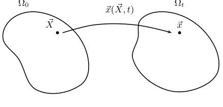
~ x(X, t~ ) Ω0
~ X
Ωt
[image:3.612.174.393.317.422.2]~x
Fig. 1.1.The flow map from the reference domain, Ω0 to the current domain,Ωt.
Here we introduce the basic mechanic background between the reference domain and the current domain at timet. The connection between these domains is the flow map. That makes it possible to do the variation with respect to domain. Let Ω0 be
the reference domain, and Ωtbe the domain at timetwith variablesX~ and~xin these
domains, respectively. Then we can obtain the flow map (trajectory) from Ω0 to Ωt
such as
~xt(X, t~ ) =~u(~x(X, t~ ), t), ~x(X,~ 0) =X.~
The deformation tensor (strain) of the flow map is given by
F(~x(X, t~ ), t) =∂~x(X, t~ )
∂ ~X
and satisfies the following transport equation:
Ft+~u· ∇F =∇~uF. (1.2)
All evolutions/dynamics are based on the above relations of flow map between the reference domain, Ω0and the domain at time t, Ωt. The deformation tensorF carries
We give an outline of this paper. In the next section, we discuss the energetic variational approaches with LAP and MDP for incompressible Navier-Stokes equa-tion. In section 3, we present two-phase flow model with diffusive interface approach in complex fluids for LAP and MDP. In applying MDP, we first manipulate the dis-sipation in the energy through Allen-Cahn equation. And then we derive a system of equations for the two-phase flow problem satisfying the modified energy equation. In section 4, we perform numerical experiments to verify the system obtained by the energetic variational approaches and discuss its numerical results. In the last section, we give a conclusion on this work.
2. Energetic Variation in Simple Fluids. In this section we consider a
sim-ple fluid model, and derive a system of equations using the energetic variational approaches with LAP and MDP. A simple fluid here means the fluid described by the incompressible Navier-Stokes equations [13, 30] which is given by
ρ(~ut+~u· ∇~u) +∇p=µ∆~u
∇ ·~u= 0 (2.1)
ρt+∇ ·(ρ~u) = 0
with a suitable boundary and initial conditions. Here, ~u is velocity field, ρ is the mass,pis the hydrostatic pressure, andµis the viscosity. Then we easily obtain the following energy equation corresponding to the incompressible Navier-Stokes equation (2.1):
d dt
Z 1
2ρ|~u|
2
dx=−
Z
µ|∇~u|2d~x. (2.2)
The energy law (2.2) can be derived directly through the system (2.1). On the other hand, according to the energetic variation approaches, we can derive the equation (2.1) from the energy equation (2.2). In (2.2) we see that the total energyEtotal and the dissipation△ for (2.1) are
Etotal=
Z 1
2ρ|~u|
2d~x,
△=
Z
µ|∇~u|2d~x, (2.3)
respectively.
We can then define the action functionalAfor the incompressible Navier-Stokes equation with the kinetic energy,
A=
Z T
0
Z
Ωt
1 2ρ|~u|
2d~xdt. (2.4)
Here we pull back the current domain, Ωt, to the reference one, Ω0, through the flow
map,~x(X, t~ ). Then the action functional is
A(~x) =
Z T
0
Z
Ω0
1
2ρ0(X~)|~xt|
2detF d ~Xdt (2.5)
where ρ0(X~) =ρ(X, t~ )|t=0 is the initial mass. Then the variation with respect to~x
which has the total energy conservation,
~
ut+~u· ∇~u=−∇p
(2.6)
∇ ·~u= 0.
Next, we apply the MDP (variation with respect to function) for the dissipation in (2.3), δδ~△u
ε=0= 0, then we obtain the Stokes equation,
µ∆~u=∇p˜
(2.7)
∇ ·~u= 0
where ˜pis a Lagrange multiplier for∇ ·~u= 0.
Therefore, we have obtained the conservative part and dissipative one in incom-pressible Navier-Stokes equation (2.1) by the energetic variational approaches, LAP and MDP, respectively.
3. Energetic Variation in Complex Fluids. We consider a complex fluids to
show the derivation of its system of equations using LAP and MDP from the energy viewpoint. There are several kinds of well-known complex fluids [7, 8, 10, 14, 25], for instance, viscoelastic material fluids with multiscale interactions, liquid crystals which is in the intermediate state between liquid and solid, magneto-hydrodynamical fluids, electro-rheological (ER) fluids, and fluid-fluid mixture models. The interac-tion/coupling between scales, or fluids, is complicated, but an essential feature of com-plex fluids. The hydrodynamic systems of comcom-plex fluids are all determined through the competition between kinetic energy and various internal elastic energies. In the meantime, the competitions are also reflected in the dissipations. Here we will use the free interface motion as an example to illustrate the underlying variational structure of these complicated systems.
We consider an immiscible two-phase flow model in complex fluids [19, 31, 32]. Let φ be a phase functionφ(~x, t) = ±1 in the incompressible fluids, and Γt = {x:
φ(~x, t) = 0} be the interface of mixture. If we consider the immiscibility of fluids, then it gives the kinematic condition on Γt, which is V~ ·~n= (~u·~n)~nwhereV~ is the
velocity of the interface Γt, and~uis the fluid velocity. In the Eulerian description, it
implies the pure transport ofφ.
φt+~u· ∇φ= 0. (3.1)
The following well-known energy, Ginzburg-Landau mixing energy, represents a competition between two fluids with their (hydro-) philic and (hydro-) phobic prop-erties:
W(φ,∇φ) = 1 2|∇φ|
2+ 1
4η2(φ 2
−1)2.
We easily see that the mixing energy functional E =λR
W d~xwhereλis a constant coefficient of the mixing energy is proportional to the area of the interface, Γt, and
the equilibrium profile of interface is tanh-like function asη→0.
The total energy is defined by the combination of the kinetic energy and the internal energy as follows:
Etotal=
Z
Ωt
1 2|~u|
2+λW(φ,
∇φ)
d~x. (3.2)
The action functionalAin terms of the flow map from the total energy (3.2) is
A(~x) =
Z T
0
Z
Ω0
1
2|~xt|
2−λ
1
2|F −1∇
~ Xφ|
2+F(φ
0)
detF
d ~Xdt. (3.3)
Notice that the term,|∇φ|2, carries all information of the configuration which is
de-termined by the deformation,F.
Remark 3.1. The expression in (3.3) includes all the kinematic transport
prop-erty of the internal variable “φ”. With different kinematic transport relations, we will obtain different action functionals, even though the energies may have the same expression in the Eulerian coordinate. This is important for dynamics for materials like liquid crystals [17, 29].
Then the LAP leads us to the following Hamiltonian system:
~
ut+~u· ∇~u+∇p=−λ∇ ·(∇φ⊗ ∇φ−W(φ,∇φ)I) (3.4)
∇ ·~u= 0 (3.5)
φt+~u· ∇φ= 0. (3.6)
Remark 3.2. The above system (3.4) – (3.6) converges to (at least formally) the
“sharp interface model” and its energy equation is
d dt
Z
1 2|~u|
2+λ
1 2|∇φ|
2+ 1
4η2(φ 2
−1)2
d~x= 0. (3.7)
It shows that the total energy of the system is conserved. The system is a Hamilto-nian system. The force, the right hand side of (3.4) is a conservative force with no dissipation of system.
Now, we consider the diffusive interface approach for immiscible two-phase flow model. The diffusive interface method is imposed by an additional dissipation term (relaxation) in the transport equation (3.6). Then we have the Allen-Cahn equation [5],
φt+~u· ∇φ=γ
∆φ− 1 η2 φ
2 −1
φ
. (3.8)
We also want to include the dissipation in flow field caused by the flow viscosity,µ. The dissipation in the diffusive interface approach is given by
△=
Z
µ|∇~u|2+λγ
∆φ− 1
η2(φ
2−1)φ
2!
d~x. (3.9)
The phase dissipation which is the second term in (3.9) is not in the form of the quadratic of the “rate” functions [22, 23, 24]. Using the equation (3.8) we can ma-nipulate the dissipation (3.9) in terms of a rate in time.
△=
Z
µ|∇~u|2+λ
γ|φt+~u· ∇φ|
2
Then the variational principle (MDP), which is known as Onsarger’s principle [22, 23, 24], δδ~△u
ε=0 = 0 with incompressibility of flow, ∇ ·~u = 0, is employed to
obtain a dissipative force.
δ△ δ~u
ε=0
= 2
Z
µ(∇~u+ε∇~v) :∇~v+λ
γ(φt+ (~u+ε~v)· ∇φ)~v· ∇φ
d~x
ε=0
= 2
Z
µ∇~u:∇~v+λ
γ(φt+~u· ∇φ)∇φ·~v
d~x (3.11)
=−2
Z
µ∆~u−λ
γ(φt+~u· ∇φ)∇φ
·~v d~x= 0.
From the above resulting equation in (3.11) we obtain the following system with dissipative force:
µ∆~u−λ
γ(φt+~u· ∇φ)∇φ=∇p˜ (3.12)
∇ ·~u= 0 (3.13)
φt+~u· ∇φ=γ(∆φ−f ′
(φ)). (3.14)
The system (3.12)–(3.14) satisfies the following energy law:
d dt
Z λ
1
2|∇φ|
2+ 1
4η2(φ 2
−1)2
d~x=−
Z
µ|∇~u|2+λ
γ|φt+~u· ∇φ|
2
d~x. (3.15)
Combine the systems, (3.4)–(3.6) and (3.12)–(3.14) obtained by LAP and MDP, respectively, we have the following system for the two-phase flow model:
~
ut+~u· ∇~u+∇p=µ∆~u−
λ
γ(φt+~u· ∇φ)∇φ (3.16)
∇ ·~u= 0 (3.17)
φt+~u· ∇φ=γ
∆φ− 1 η2(φ
2 −1)φ
. (3.18)
The most amazing fact from the above derivation is the dissipation force from MDP in (3.12). The dissipative term,−γλ(φt+~u· ∇φ)∇φin (3.12), is exactly same as the
conservative term,∇ ·(∇φ⊗ ∇φ−W(φ,∇φ)I) from LAP in (3.4).
Moreover, asη→0, this is exactly the surface tension force on the interface [31]. This system (3.16)–(3.18) satisfies the dissipative energy law.
d dt
Z
1 2|~u|
2+λ
1 2|∇φ|
2+ 1
4η2(φ 2
−1)2
d~x
(3.19) =−
Z
µ|∇~u|2+λ
γ|φt+~u· ∇φ|
2
d~x.
This procedure using the energetic variation, especially, MDP sometimes gives advan-tage in designing numerical algorithms. If the dissipative force in (3.16) is substituted by the conservative force in (3.4), then the following equation is obtained
~ut+~u· ∇~u+∇p=µ∆~u−λ∇ ·(∇φ⊗ ∇φ−W(φ,∇φ)I). (3.16′)
Moreover, the system (3.16′
), (3.17), (3.18), satisfies the following energy law:
d dt
Z 1
2|~u|
2+λ
1 2|∇φ|
2+f(φ)
d~x=−
Z
µ|∇~u|2+λγ|∆φ−f′(φ)|2
d~x(3.20)
where f(φ) = 41η2(φ2−1)2. Since in derivation of the energy (3.20), the equation
(3.18) is multiplied by ∆φ− η12(φ2−1)φ, a numerical algorithm to solve (3.16
′ ), (3.17), (3.18), requires a high order approximation for the phase field solution to pre-serving the energy (3.20). On the other hand, to derive the energy (3.19) we multiply
φt+~u· ∇φ, thus, in solving the system (3.16)–(3.18) a numerical algorithm can be
implemented in a low order approximation forφto preserve the energy (3.19).
Remark 3.3. It may be strange that in the equation (3.16)–(3.18) the surface
tension can be viewed as a dissipative force. In fact, this is due to the relaxation of the φ equation. To see this let’s look at the simple viscoelastic fluids. For instance, we consider a incompressible viscoelastic complex fluid model with the elastic energy,
W(F) =|F|2 [18]. Then the energy equation is given by
d dt
Z
1 2|~u|
2+1
2|F|
2
d~x=−
Z
µ|∇~u|2d~x. (3.21)
The following system of equations satisfies the energy law (3.21):
~
ut+~u· ∇~u+∇p=µ∆~u+∇ · WFF −T
(3.22)
∇ ·~u= 0 (3.23)
Ft+~u· ∇F =∇~uF (3.24)
with det(F) = 1. The dissipation in (3.21) does not include the rate functions in terms ofF. The forceWFF−T is only a conservative force. The MDP can be applied
only on~uvariable to obtain the viscosity term,∆~u. If we add an artificial term∆F
like in viscosity method for hyperbolic system into (3.24) without further discussion of the physical meaning on this artificial “viscosity” term (as an approximation of the original equation (3.24)), then the resulting equation is
Ft+~u· ∇F =∇~uF+ε2∆F. (3.24′)
Now, we can apply the MDP for the system (3.22),(3.23), (3.24′
). Moreover, the system (3.22), (3.23), (3.24′
), satisfies the following energy equa-tion:
d dt
Z 1
2|~u|
2+1
2|F|
2
d~x=−
Z
µ|∇~u|2+ε2|∇F|2
d~x. (3.25)
The extra dissipation onF in (3.25) can be written from (3.24′
) in terms of a “rate” function, using the Riesz transformation,R which is defined by
R[g](~x) =cn
Z (~x
−~y)
|~x−~y|ng(~y)d~y
wheren > 2 is the space dimension, and cn is a constant depended on n [28]. Then
the resulting energy equation is
d dt
Z 1
2|~u|
2+1
2|F|
2
d~x=−
Z
µ|∇~u|2+ε2R[Ft+~u· ∇F− ∇~uF]2
andWFF−T can also be derived from MDP.
In the next section, we present numerical experiments, and discuss its results as a verification for the system (3.16)–(3.18) driven by the energetic variational approach.
4. Numerical Simulations. The numerical experiments for two-phase flow
problem modeled by diffusive interface approach are carried out with finite element methods [4, 6, 11] for the system (3.16)–(3.18). We discuss the numerical results and algorithms to solve the system. We here emphasize again that if the system (3.16′
), (3.17), (3.18), is employed to solve two-phase flow problem then the finite element space for the phase field solution, φ, has to have at least H2-regularity to preserve the dissipative energy law (3.20), for instance,P2 finite element space, or biquadratic
element space [20, 21]. HerePk means the space of polynomials up to orderk. But it
causes an expensive computational costs. On the other hand, the energy law (3.19) for the system (3.16)–(3.18) allows us to employ a lower order finite element space for the phase solution, for instance,P1 element.
The finite element spaces and mesh generations are implemented by the Free-Fem++ [12]. In discretization, the superscript, n, means the time step, and the subscript,h, is for the finite dimensional variable or space. The following finite element spaces are used for simulations:
~
uh∈Vh= (P1⊕bubble)2 (4.1)
ph∈Wh=P1 (4.2)
φh∈Qh=P1 (4.3)
for the finite dimensional solution pair (~uh, ph, φh) rather than high order element,
for instance,P2 forφh.
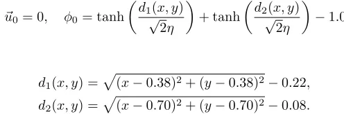
The computational domain is the unit square. The initial velocity field is~u0= 0,
and the initial phases are given by
φ0= tanh
d1(x, y) √
2η
+ tanh
d2(x, y) √
2η
−1.0, (4.4)
where d1, d2 are the distance functions from the circle centered at (0.38,0.5) radius
r= 0.11 and at (0.62,0.5) radiusr= 0.11, respectively. The explicit forms ofd1and
d2are given as follows:
d1(x, y) =
p
(x−0.38)2+ (y−0.5)2−0.11,
d2(x, y) =
p
(x−0.62)2+ (y−0.5)2−0.11.
We can easily see the fact that the initial value (4.4) is an approximation of the following phase field:
φ0=
(
−1, inside region of circles
1, outside region of circles. (4.5)
Remark 4.1. Since the system (3.16)–(3.18) is highly nonlinear system
consist-ing of the incompressible Navier-Stokes equation with the stress term and Allen-Cahn equation, there exist many finite element approximation schemes, for instance, the characteristic Galerkin finite element method gives an approximation for the convec-tion term in Navier-Stokes equaconvec-tion.
~
ut+ (~u· ∇)~u≈
~
unh+1−~unh(~x−~unh∆t)
∆t (4.6)
gives a quadratic convergence order [5, 9, 26]. Also one can use the stabilized semi-implicit scheme for Allen-Cahn equation (3.18) [19]. But the approximation (4.6) for the convection term sometimes breaks the dissipative energy law. In fact, when we used this approximation in the numerical examples of Figure (4.1) and (4.3) we observed that the dissipative law of the total energy is violated during the simulations, especially in the beginning of the time.
To preserve the finite dimensional dissipative energy law an explicit-implicit sec-ond order temporal discretization algorithm is employed for numerical experiments [16, 17]. The variational formulation for the solution (~unh+1, pnh+1, φnh+1) using the explicit-implicit scheme as follows:
(˜~unh,t+1, ~vh) +
3 ~ un
h−~un −1
h
2 · ∇
~ u
n+1 2
h , ~vh
+
1
2
∇ ·3~u
n h−~un
−1 h 2 ~u n+1 2
h , ~vh
−(p
n+1 2
h ,∇ ·~vh) =−(µ∇~u n+1
2
h ,∇~vh)−
λ γ
˜
φnh,t+1∇
3
φnh−φnh−1
2
, ~vh
(4.7) −λ γ ~ u n+1 2
h ,∇
3φn h−φn
−1
h
2 ∇
3φn h−φn
−1
h
2
, ~vh
for all~vh∈Vh,
(∇ ·~u
n+1 2
h , wh) = 0 for allwh∈Wh, (4.8)
( ˜φnh,t+1, qh) +
~ u n+1 2 h , 3
φnh−φnh−1
2
qh
(4.9) =−γ∇φ
n+1 2
h ,∇qh
− γ
η2(fh(φ
n
h, φnh+1), qh) for allqh∈Qh
where
fh(φnh, φnh+1) =
(
|φnh+1|2−1) + (|φn h|2−1)
2 φ n+1 2 h , ˜ ~
unh,t+1=~u
n+1
h −~unh
∆t , ~u
n+1 2
h =
~
unh+1+~unh
2 , φ˜
n+1
h,t =
φnh+1−φnh
∆t , φ
n+1 2
h =
φnh+1+φnh
2 ,
(·,·) is the inner product operator, and ∆t is the time step for simulations. Here we employ the penalty method for Navier-Stokes equation [30, 11, 4]. Then the equation (4.8) is substituted by
(∇ ·~u
n+1 2
h , wh) +ε(p n+1
2
h , wh) = 0 for allwh∈Wh (4.8′)
whereεis a positive small constant, 0< ε <<1. In numerical simulations, we usually takeε= 10−6. Then the variational problem, (4.7), (4.8′
), (4.9), satisfies the following finite dimensional dissipative energy law:
Z 1
2|~u
n+1
h |
2+
λ 1
2|∇φ
n+1
h |
2+ 1
4η2|φ
n+1
h
2 −1|2
d~x h,t (4.10) =− Z (
µ|∇~unh+1|2+ε|φ
n+1 2
h |
2+λ
γ ˜
φnh,t+1+ (~u
n+1 2
h · ∇)
3 φn
h−φn −1 h 2 2) d~x.
Plot of Interfaces and Flow Fields at Time =0
0.2 0.3 0.4 0.5 0.6 0.7 0.8 0.2
0.3 0.4 0.5 0.6 0.7 0.8
Plot of Interfaces and Flow Fields at Time =0.1
0.2 0.3 0.4 0.5 0.6 0.7 0.8 0.2
0.3 0.4 0.5 0.6 0.7 0.8
Plot of Interfaces and Flow Fields at Time =0.2
0.2 0.3 0.4 0.5 0.6 0.7 0.8 0.2
0.3 0.4 0.5 0.6 0.7 0.8
Plot of Interfaces and Flow Fields at Time =0.4
0.2 0.3 0.4 0.5 0.6 0.7 0.8 0.2
0.3 0.4 0.5 0.6 0.7 0.8
Plot of Interfaces and Flow Fields at Time =0.7
0.2 0.3 0.4 0.5 0.6 0.7 0.8 0.2
0.3 0.4 0.5 0.6 0.7 0.8
Plot of Interfaces and Flow Fields at Time =1
0.2 0.3 0.4 0.5 0.6 0.7 0.8 0.2
[image:11.612.141.443.100.528.2]0.3 0.4 0.5 0.6 0.7 0.8
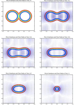
Fig. 4.1.The time evolution results (merging effect) of phase field and velocity field from
left to right and top to bottom (t= 0.0,0.1,0.2,0.4,0.7,1.0and∆t= 0.001).
We want to point that it is difficult/challeging to obtain the optimal order er-ror estimate of the variational problem (4.7), (4.8′), (4.9). In [16, 17], the authors only present the convergence estimate for the explicit-implicit scheme in fixed point nonlinear iteration under the certain condition.
The numerical results of time evolution for the phase field and the velocity field in variational problem (4.7), (4.8′), (4.9) are presented in Figure 4.1 through the contour plots at time,t= 0.0,0.1,0.2,0.4,0.7,1.0, and the total energy and the kinetic energy in Figure 4.2. These numerical results are demonstrating that the lower order finite
0 0.2 0.4 0.6 0.8 1 1.2 0
0.002 0.004 0.006 0.008 0.01 0.012 0.014
Time : t
Energy
Energy Dissipation : Merging Effect
Total Energy Mixing Energy Kinetic Energy
0 0.2 0.4 0.6 0.8 1 1.2 0
0.2 0.4 0.6 0.8 1 1.2 1.4 1.6 1.8x 10
−6
Time : t
Energy
[image:12.612.119.466.96.239.2]Kinetic Energy Evolution : Merging Effect
Fig. 4.2. The total energy dissipation (left) and the kinetic energy (right) of merging phenomena in two-phase interface model.
element space for phase field satisfactorily works to catch the merging phenomena of two-phase flow model with the system (3.16)–(3.18). The left picture in Figure 4.2 shows the total energy dissipation. The elastic internal energy is dominant in the simulation, that is, the kinetic energy is very small quantity. The right picture in Figure 4.2 shows the evolution of kinetic energy. In the beginning time the kinetic energy is increasing until time t = 0.1 and then decreasing because the flow fields effect induced by the motion by mean-curvature is strong in the beginning time. As the interface becomes smooth, the motion by mean-curvature decreases. After the merging region of interface becomes flat, the kinetic energy almost does not change until time,t= 0.9 and then rapidly vanishes.
The next simulation is set by the following initial conditions:
~
u0= 0, φ0= tanh
d1(x, y) √
2η
+ tanh
d2(x, y) √
2η
−1.0 (4.11)
with
d1(x, y) =
p
(x−0.38)2+ (y−0.38)2−0.22,
d2(x, y) =
p
(x−0.70)2+ (y−0.70)2−0.08.
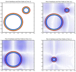
The results of interface evolution with the flow field induced by surface tension of the interface are presented in Figure 4.3, and its total energy and kinetic energy in Figure 4.4. In Figure 4.3 the results also works very well to catch the behavior of interfaces. The interface in shape of small circle is dissipated faster than that of large circle. In the simulation, the mixing energy dissipation shows a dominant behavior similar to the previous merging effect. We also observe that at the vanishing time, aroundt= 0.25, of the small interface, the total energy is rapidly decreasing because its interface is vanishing, dramatically.
5. Conclusion. We employed the energetic variation approaches in
[image:12.612.166.414.430.512.2]Plot of Interfaces and Flow Fields at Time =0
0.1 0.2 0.3 0.4 0.5 0.6 0.7 0.8 0.9 0.1
0.2 0.3 0.4 0.5 0.6 0.7 0.8 0.9
Plot of Interfaces and Flow Fields at Time =0.2
0.1 0.2 0.3 0.4 0.5 0.6 0.7 0.8 0.9 0.1
0.2 0.3 0.4 0.5 0.6 0.7 0.8 0.9
Plot of Interfaces and Flow Fields at Time =0.4
0.1 0.2 0.3 0.4 0.5 0.6 0.7 0.8 0.9 0.1
0.2 0.3 0.4 0.5 0.6 0.7 0.8 0.9
Plot of Interfaces and Flow Fields at Time =2
0.1 0.2 0.3 0.4 0.5 0.6 0.7 0.8 0.9 0.1
[image:13.612.141.446.96.385.2]0.2 0.3 0.4 0.5 0.6 0.7 0.8 0.9
Fig. 4.3.The time evolution results of phase field and velocity field from left to right and
top to bottom (t= 0.0,0.2,0.4,2.0and∆t= 0.001).
“variables”. If this is the case, then the conservative force in hydrodynamic system is consistent with the dissipative force. As presented in this paper, this procedure, MDP plays an important role in designing numerical algorithms to solve the hydrodynamic complex fluid problem. Through MDP, a system of equations can be reformulated to employ a numerical algorithm with lower order element to solve a complex fluid problem, and still preserve the dissipation energy law.
Finally, we want to point out that the system derived by MDP does give rise to a different challenge in numerical analysis. An additional time derivative term and convection terms in hydrodynamic force have appeared in the system of equations. It is important (difficult) to obtain an error estimate of optimal order for the finite element method. One of our next objectives in this area is to find other discretization schemes to solve the system and prove the optimal order of convergence.
REFERENCES
[1] D.M. Anderson, G.B. McFadden and A.A. Wheeler,Diffuse-interface Methods in Fluid Mechanics, in: Annual Review of Fluid Mechanics, Vol. 30, Annual Review, Palo Alto CA, (1998), pp.139–165.
[2] R.B. Bird, R.C. Armstrong, and O. Hassager,Dynamics of Polymeric Fluids, Vol. 1, Fluid Mechanics. John Wiley & Sons, New York, (1977).
[3] R.B. Bird, O. Hassager, R.C. Armstrong, and C.F. Curtiss, Dynamics of Polymeric
0 0.5 1 1.5 2 0
0.002 0.004 0.006 0.008 0.01 0.012 0.014 0.016 0.018
Time : t
Energy
Energy Dissipation : Vanishing Effect
Total Energy Mixing Energy Kinetic Energy
0 0.5 1 1.5 2 0
0.5 1 1.5 2 2.5
3x 10
−6
Time : t
Energy
[image:14.612.119.464.96.239.2]Kinetic Energy Evolution : Vanishing Effect
Fig. 4.4. The total energy dissipation (left) and the kinetic energy (right) of vanishing phenomena in two-phase interface model.
Fluids, Vol. 2, Kinetic Theory. John Wiley & Sons, New York, (1977).
[4] F. Brezzi, and M. Fortin,Mixed and hybrid finite element methods, Springer-Verlag, New York, 1991.
[5] J.W. Cahn, and S.M. Allen,A Microscopic Theory for Domain Wall Motion and Its Ex-perimental Verification in Fe-Al Alloy Domain Growth Kinetics, J. Phys. Colloque C7, (1978), C7–C51.
[6] P.G. Cialet,The finite Element Method for Elliptic Equations, North-Holland, Amsterdam (1978).
[7] P.G. De Gennes, and J. Prost,The Physics of Liquid Crystals, second ed., Oxford Science Publications, Oxford, (1993).
[8] M. Doi and S.F. Edwards,The Theory of Polymer Dynamics, Clarendon Press, Oxford, UK, (1986).
[9] J. Douglas, and T.F. Russell,Numerical Methods for convection Dominated Diffusion Prob-lems based on Combining the method of characteristics with Finite Element Methods of Finite Difference Method, SIAM J. Numer. Anal., 19(1982), pp.871–885.
[10] J. Erickson,Conservation Laws for Liquid Crystals, Trans. Soc. Rheol. 5(1961), pp. 22–34. [11] V. Girault, and P.A. Raviart,Finite element methods for Navier-Stokes equations,
Springer-Verlag, Berlin, (1986).
[12] F. Hecht, O. Pironneau, A. Le Hyaric, and K. Ohtsuka, FreeFem++, http://www.freefem.org, (2007).
[13] D. Jacqmin,Calculation of Two-Phase Navier-Stokes Flows Using Phase-Field Modeling, J. Comput. Phys., 155(1999), pp.96–127.
[14] R.G. Larson,The Structure and Rheology of Complex Fluids, Oxford University Press, New York, (1999).
[15] F.H. Lin, and C. Liu,Global Extistence of Solutions for the Erickson Leslie-system, Arch. Rat. Mech. Anal. 154(2)(2001), pp. 135–156.
[16] P. Lin, and C. Liu,Simulation of Singularity Dynamics in Liquid Crystal Flows: aC0
Finite Element Approach, J. Comput. Phys., 215(2006), pp.348–362.
[17] P. Lin, C. Liu, and H. Zhang,An Energy Law Preserving C0
Finite Element Scheme for Simulationg the Kinematic Effects in Liquid Crystal Flow Dynamics, J. Comput. Phys., 227(2007), pp.1411–1427.
[18] F.H. Lin, C. Liu, and P. Zhang,On Hydrodynamics of Viscoelastic Fluids, Comm. Pure Appl. Math., LVIII(2005), pp. 1–35
[19] C. Liu, and J. Shen,A Phase Field Model for the Mixture of Two Incompressible Fluids and Its Approximation by a Fourier-Spectral Method, Physica D, 179(2003), pp.211–228. [20] C. Liu, and N.J. Walkington, Approximation of Liquid Crystal Flows, SIAM J. Numer.
Anal., 37(3)(2000), pp.725–741.
[21] C. Liu, and N.J. Walkington,Mixed Methods for the Approximation of Liquid Crystal Flows, M2AN, 36(2)(2002), pp.205–222.
[22] L. Onsager,Reciprocal Relations in Irreversible Processes I, Phys. Rev. 37(1931), pp.405–426. [23] L. Onsager,Reciprocal Relations in Irreversible Processes II, Phys. Rev. 38(1931), pp. 2265–
[24] L. Onsager, and S. Machlup,Fluctuations and Irreversible Processes, Phys. Rev. 91(1953), pp. 1505–1512.
[25] R. Owens, and T. Phillips,Computational Rheology, Imperial College Press, London, (2002). [26] O. Pironneau,On the Transport-Diffusion Algorithm and Its Applications to The
Navier-Stokes Equations., Numer. Math., 38(1982), pp.309–332.
[27] H. Rui, and M. Tabata,A Second Order Characteristic Finite Element Scheme for Convection Diffusion Problems, Numer. Math., 92(2002), pp.161–177.
[28] E.M. Stein,Singular Integrals and Differentiability Properties of Functions, Princeton Uni-versity Press, (1970).
[29] H. Sun, and C. Liu,On Energetic Variational Approaches in Modeling the Nematic Liquid Crystal Flows, Discrete and Continuous Dynamical Systems, 23(2009), pp.455–475. [30] R. Temam,Navier-Stokes Equations, North-Holland, Amsterdam, (1977).
[31] X.F. Yang, J.J. Feng, C. Liu, and J. Shen,Numerical Simulations of Jet Pinching-off and Drop Formation Using An Energetic Variational Phase-Field Method, J. Comput. Phys., 218(2006), pp.417–428.
[32] P.T. Yue, C.F. Zhou, J.J. Feng, C.F. Ollivier-Gooch, and H.H. Hu,Phase-field simula-tions of Interfacial Dynamics in Viscoelastic Fluids Using Finite Elements with Adaptive Meshing, J. Comput. Phys., 219(2006), pp.47–67.