Systems & Control Letters 48 (2003) 15–25
www.elsevier.com/locate/sysconle
Overparameterised adaptive controllers can reduce
non-singular costs
F. Beleznay
1, M. French
∗Department of Electronics and Computer Science, University of Southampton, Southampton SO17 1BJ, UK Received 25 March 2002; received in revised form 23 July 2002; accepted 13 August 2002
Abstract
By means of two examples we show that non-singular costs can been reduced for adaptive controllers by overparameterising the estimators. The examples are for scalar and second order systems respectively. In the second example the tuning function design and the overparameterised adaptive backstepping design are compared. In both cases a system is constructed for which the overparameterised design is superior w.r.t. a non-singular measure of transient performance.
c
2002 Published by Elsevier Science B.V.
Keywords:Overparameterisation; Back stepping; Performance
1. Introduction
Overparameterisation in adaptive controllers has of-ten been considered to be a undesirable design feature. Generally overparameterisation leads to controllers of higher dynamic order with more complex dynamics and hence there is often a concern about a possi-ble loss of robustness. There are a few results which partially support this intuitive claim, for example [7] presents concrete results showing parameter conver-gence for systems with fewer parameters, hence GAS of the closed loopand robustness to bounded distur-bances. Often, informal reasonings for the need to re-duce over-parameterisation are given as follows: as the dimensionality of the parameter space increases, parameter convergence is harder to achieve, which in
∗Corresponding author. Tel.: 8059-2688; fax:
+44-23-8059-4498.
E-mail addresses:[email protected](F. Beleznay),
[email protected](M. French).
1Present address: Department of analysis, EBotvBos Lorand
Uni-versity, Budapest, Hungary.
turn can lead to robustness problems. Alternatively, it can be reasoned that because the parameter space is larger, the transient is larger. However, these argu-ments do not necessarily hold upto close scrutiny. For example, in the latter case, it is well known within the machine learning community that the size of parame-ters can be more critical for learning performance than the number of parameters, see e.g. [1]. Although the problem considered in [1] is not directly analogous, it exposes the weakness of the intuitive argument, by suggesting the ‘size’ of a learning problem may be dictated by measures of ‘size’ which are not as elementary as parameter counts.
On the other hand, overparameterisation can give the controller beneGcial extra degrees of freedom in the design, see e.g. [5]. We exploit these extra degrees of freedom in the constructions which fol-low, which show thatthe orthodoxy that one should not over-parameterise,is not,in general,valid.2 In
2Related results in the context of function approximator based
designs can be found in [4]. 0167-6911/03/$ - see front matter c2002 Published by Elsevier Science B.V.
particular, we give two examples of systems and con-trollers whereby a sensible closed loopcost is lower for the overparameterised design. In this paper, we will consider the non-singular cost functionals
P=qTxL∞+ruL∞;
P=qTx2
L2+ruL∞; (1)
wherexis the system state,u is the control and q; r
are weighting parameters. We observe that it is critical to introduce a penalty on control eLort in order to have a well-posed problem—the classes of systems considered in this paper are minimum phase and admit high gain solutions, which by trajectory initialisation [8] can yield arbitrarily small output responses at the price of high control eLort. Furthermore, we need to be able to develop both upper and lower bounds for these costs. There are general results available for bounding the output transients of adaptive controllers, see e.g. [8], but in general the problem of bounding the control eLort is much harder, however see e.g. [3,2].
The Grst example is a scalar system, and it is shown that the transient performance of a standard adaptive controller is improved when the estimator is over-parameterised. The essence of the example is that if an estimator has been driven to an overly high value (in this case by a large state initial condition), then it is desirable to ‘forget’ the ‘large’ value and restart adapting from a low value. Overparameterisation allows us to do this.
We then consider systems in strict feedback form, with adaptive backstepping controllers [6]. It is well known that such controllers are overparameterised (if
nis the order of the system andpis the number of pa-rameters then there aren(n+ 1)p=2 estimators). The tuning function design [7] eliminates the overparame-terisation completely. The second contribution of this paper is to construct a situation in which the over-parameterisation of the adaptive backstepping design leads to a superior transient response to that of the tuning function design.
In particular, we construct a second-order system for which the following holds. Suppose we optimize the controllers for regulation to a pointyr=b. Then
the closed loopyield the same cost for either con-troller when applied with yr =b, whilst the
adap-tive backstepping controller has superior performance
when yr =a. We interpret this result in a simple
probabilistic setting. We are not in any way claiming that the adaptive backstepping design is superior to the tuning function design in general, as we fully ex-pect that examples showing the contrary relationship between performance can also be established.
Ideally one would like to have results which fully characterise when to over-parameterise or not, or, more speciGcally, when to use the adaptive back-stepping design and when to use the tuning function design. However, this remains an challenging open area of research. It is likely to be extremely diOcult to achieve such characterisations, such an analysis would have to contend with the complexities of the backstepping transformations, the non-optimality of the controllers and the non-singularity of the cost, all of which lead to complex dynamics and to an extremely complex problem. An indication of the complexity of this problem may be obtained by con-sidering the proof of Theorem 2 below. Whilst the system nonlinearities were chosen to simplify the problem as much as possible, the argument remains delicate.
Whilst the examples in this paper are extremely specialized, the paper makes a practical contribution: when designing adaptive controllers, do not dismiss over-parameterised designs; they may have superior performance!
2. A motivating scalar example
Consider the system
(x0; ): ˙x=f(x) +u; x(0) =x0; (2)
where ∈Ris an unknown parameter, x; u are real scalar valued signals, and f:R → R is a function which is of the form
f(x) =1(x) +2(x) =1(x) +x (x); (3)
where1, have the properties
1. 1 is continuous with support in (−∞;1), and
1(0)= 0.
2. is continuous and non-negative with support in (3;∞), and (x) = 1∀x¿4.
signals bounded. Consider the following two con-trollers:
u() :u=−fˆ (x)−x; ˙ˆ
=xf(x); ˆ(0) = 0; (4)
o(
1; 2) :u=−ˆ11(x)−ˆ22(x)−x;
˙ˆ
1=1x1(x); ˆ1(0) = 0;
˙ˆ
2=2x2(x); ˆ2(0) = 0: (5)
Both controllers achieve stability ∀x0; ∈R. The
proof is standard and can be achieved by consider-ing the quadratic Lyapunov functions Vu = 12x2 + (1=2)( − ˆ)2; V
o = 12x2 + (1=21)( − ˆ1)2 +
(1=22)(−ˆ2)2, respectively.
We measure transient performance by the cost
P((; x0); ()) =x2L2+uL∞ (6)
and it is convenient to deGne P|[0;t] =x2L2[0;t] +
uL∞[0;t]; Po=P((; x0); o(; )); Pu=P((; x0);
u()).
The result for this section is as follows:
Theorem 1. For all ¿0; ∈R, lim
x0→∞P
u−Po=∞: (7)
The theorem therefore states that the diLerence between the basic design and its overparameterised variant becomes arbitrarily large as the size of the initial condition increases. In particular, the overpa-rameterised design has superior performance.
Proof. Consider(; x0) with either o or u.
Sup-posex0¿4. Then by the fact thatx(t)→0 ast→ ∞,
and the deGnition of1; 2 it follows that there is a
unique timet∗at whichx(t∗)=2, since whenx(t)=2,
then ˙x=−x ¡0. Now observing that on [0; t∗]u; o are identical, it follows that
Pu|
[0;t∗]=Po|[0;t∗]: (8)
Now consider ((; x0); o(; )). Note that ˆ2 is an
increasing function, as its derivative is non-negative. We now claim that ˆ2(t∗) → ∞ as x0 → ∞.
Suppose the contrary, i.e. that there exists M ¿0, such that for some divergent sequence of points {x0i}i¿1; ˆ2(t∗)6M. Lett∗∗=inf{t¿0 :x(t)=4},
and note that 06ˆ2(t∗∗)6ˆ2(t∗)6M. Now
t∗∗
0 x 2dt
=
t∗∗
0 −
˙
Vdt=V(0)−V(t∗∗)
¿12x2 0i−8 +
1 22(
2+ (+M)2)→ ∞
asi→ ∞: (9)
Now, since ˙V=−x2, we have
ˆ
2(t∗)¿ˆ2(t∗∗)
=
t∗∗
0
˙ˆ
2dt=
t∗∗
0 2x
2(t) dt→ ∞
asi→ ∞: (10)
This is a contradiction, hence ˆ2(t∗) → ∞as x0 →
∞. The same argument for ((; x0); u()) shows
ˆ
(t∗)→ ∞asx0→ ∞.
It can easily be seen for the overparameterised con-trollero, thatuL∞[t∗;∞) is independent ofx0 (this can be shown formally by considering r(0; ) be-low), whilst
uL∞[0;t∗]¿| −ˆ2(t∗∗)2(4)−4|
¿4 ˆ2(t∗∗) + 4→ ∞ asx0→ ∞:
(11) It thus follows that for largex0, the supremum foruis
attained on [0; t∗], and in particular it then follows for
largex0, thatuL∞ foruis greater than or equal to
that foro. Sincex2
L2=x2L2[0;t∗]+x2L2[t∗;∞), it
then follows that for suOciently largex0,
Pu−Po¿ ∞ t∗ x
2
udt−
∞
t∗ x
2
odt
+uuL∞(R+)− uoL∞(R+)
¿
∞
t∗ x
2
udt−
∞
t∗ x
2
odt: (12)
We now claim thatt∞∗ x2udt→ ∞asx0→ ∞, whilst
∞
then follows. To showt∞∗ x2odtis independent from
x0 it suOces to observe that the controller on [t∗;∞)
is simplyr(0; ) for o (and r( ˆ(t∗); ) foru), wherer(·;·) is deGned
r(
0; ):u=−ˆ 1(x)−x;
˙ˆ
=x1(x) ˆ(t∗) =0: (13)
Clearly r(0; ) is independent of x0, hence so is
Po|
[t∗;∞). It remains to show thatt∞∗ xu2dt → ∞ as
x0 → ∞. By taking0= ˆ(t∗)→ ∞as x0 → ∞, it
suOces to show thatr(0; ) causes∞
t∗ x2dt to
di-verge as0→ ∞. Since1(0)= 0 and ˆ; is scalar,
it follows that ˆ→ast→ ∞[7]. Now
∞
t∗ x
2dt= ∞
t∗ −
˙
Vdt=V(t∗)−V(∞)
= 2 +21(−0)2→ ∞
as0→ ∞; (14)
as required, thus completing the proof.
3. Modication of the adaptive backstepping design
Consider a system in parametric strict feedback form, denoted by(; 1; : : : ; n;x0)
˙
x1=x2+T1(x1);
... x(0) =x0;
˙
xn−1=xn+Tn−1(x1; : : : ; xn−1);
˙
xn=u+Tn(x1; : : : ; xn);
y=x1; (15)
wherexi:R+→R,∈Rmfor somemis an unknown
parameter and i:Ri → Rm. Our goal is to com-pare two designs that regulate the output signalyto some constantyr (i.e. limt→∞y(t) =yr) using a
con-trollerwith inputx1; : : : ; xnand outputu:R+→R.
The Grst design we consider is a modiGcation of the overparameterised adaptive backstepping controller
introduced in [6], and e.g. in [8, Theorem 3.5]. It is straightforward to observe that there is no need to have one adaptation gain matrix. We can introduce dif-ferent matrices for the diLerent estimates ofto have more design freedom. This way we can get the follow-ing slightly modiGed adaptive backsteppfollow-ing controller for which the claims of [8, Theorem 3.5] are still true. We also add terms to be able to use the controller for tracking a reference signalyr(t). We denote this
con-troller byAB(1; : : : ; n; yr)
u=n(x1; : : : ; xn;ˆ1; : : : ;ˆn; yr(0); : : : ; yr(n−1)) +yr(n);
˙ˆ
i=i
i−i−1
j=1
@i−1
@xj j
zi; ˆi(0) = 0;
zi=xi−y(ri−1)
−i−1(x1; : : : ; xi−1;ˆ1; : : : ;ˆi−1; yr(0); : : : ; yr(i−2));
i=−cizi−zi−1−
i−i−1
j=1
@i−1
@xj j
T
ˆ
i
+i−1 j=1
@i−1
@xj xj+1+
@i−1
@yr(j−1) y (j) r
+@i−1
@ˆj j j− j−1
k=1
@j−1
@xk k
zj
; (16)
where ci¿0;ˆi:R+ → Rm and i =Ti ¿0. The second controller we consider is the following version of the tuning function controller of [8], which we de-note byTF(; yr). The original design is summarized
in Table 4.1 of [8]. To be able to compare the two designs we set the nonlinear damping term%= 0:
u=n(x1; : : : ; xn;; yˆ (0)r ; : : : ; y(rn−1)) +y(rn);
˙ˆ
=n
i=1
i−i−1
j=1
@i−1
@xj j
zi; ˆ(0) = 0;
i=−cizi−zi−1−
i−i−1
j=1
@i−1
@xj j
T
ˆ
+ i
j=1
@i−1
@xj xj+1+
@i−1
@y(rj−1)y (j) r
+@i−1
@ˆ j−
j−1
k=1
@j−1
@xk k
zj
+ i−1
k=2
@k−1
@ˆ
i−i−1
j=1
@i−1
@xj j
zk; (17)
whereci¿0; ˆ:R+→Rmand=T¿0. The cost
function we use to measure the performance of the system, controller pair (; ) is
P(; ) =yL∞+&1x2L∞+&2uL∞ (18)
for some constants&1; &2¿0. We Gx theci’s through-out the paper. Before stating the main result, we recall a deGnition. A controller is said to be '-suboptimal ifP(; ( '))6inf ¿0P(; ( )) +', where =
in the tuning function case, and = (1; : : : ; n) in the adaptive backstepping case. We will prove the following theorem:
Theorem 2. Suppose that the design objective is to regulate the output signal to a constantyr∈[a; b]for
some interval [a; b]. Then there exists a system
of degree two,an interval[a; b]and constants&1; &2,
such that the following hold. There is'∗¿0such that
for all0¡ ' ¡ '∗,if
AB(1; 2; b)is an'-suboptimal
adaptive backstepping controller foryr=b,then with
=2,TF(; b)is an'-suboptimal tuning function
controller foryr=b.Moreover
P(; AB(1; 2; b)) =P(; TF(; b)); (19)
but
P(; AB(1; 2; a))¡ P(; TF(; a)): (20)
Remark. The theorem can be interpreted in the fol-lowing manner. Suppose we do not knowyr a priori,
but we expectyr=bwith high probability. We would
therefore optimize foryr=b. If this expectation is
in-correct and in factyr =awith high probability, then
we would be in precisely the situation of the theorem.
By applying continuity arguments, we should there-fore expect that we were in a situation where the con-troller will be asked to control to yr =a with high
probability, but with a small probability of yr =b,
then the adaptive backstepping controller would give the lower expected cost. This type of scenario can be envisaged in robotics whereby a robot may be opti-mized for large movements, and occasionally asked to complete small movements.
4. Example
First we look at the design forn= 2 andyr(t) = 0.
We will consider the following system(1; 2; ;x0)
˙
x1=x2+1(x1);
˙
x2=u+2(x1; x2); x(0) =x0;
y=x1; (21)
where x1; x2 : R+ → R, ∈R+ and i:Ri → R. The tuning function recursion using c1 = 1 and
c2 = 3 results the following closed loopsystem
((1; 2; ;x0); TF(;0)):
˙
x1=x2+1;
˙
x2=u+2; x(0) =x0;
˙ˆ
=(2+1+1ˆ 1)(x2+x1+1ˆ)
+1x1; ˆ(0) = 0;
y=x1;
u=−4x2−4x1−41ˆ−1xˆ 2
−
1ˆ 1ˆ−2ˆ−11x1
−1(2+1+1ˆ 1)(x2+x1+1ˆ); (22)
where ¿0 is the design constant. The modiGed adaptive backstepping recursion using c1 = 1 and
((1; 2; ;x0); AB(1; 2;0)):
˙
x1=x2+1;
˙
x2=u+2; x(0) =x0;
˙ˆ
1=11x1; ˆ1(0) = 0;
˙ˆ
2=2(2+1+1ˆ11)(x2+x1+1ˆ1);
ˆ
2(0) = 0;
y=x1;
u=−4x2−4x1−31ˆ1−1ˆ2−1ˆ1x2
−
1ˆ11ˆ2−2ˆ2−111x1; (23)
where1; 2¿0 are the design constants.
Let b(x) :R → R be any twice diLerentiable “bump” function satisfying the following conditions:
b(x) = 0 for x6 − 1
2 and x¿12, b(0) = 1 and
06b(x)61 for−1
26x612. Let s(x) :R → Rbe
any twice diLerentiable “step” function satisfying the following conditions:s(x) = 0 forx6−1
2; s(x) = 1
forx¿1
2 and 06s(x)61 for−126x612. We will
consider systems(1; 2; ;x0) deGned by
1(x1) =−Hb(x1−32) (24)
for someH ¿0,
2(x1; x2) = (−Ks(x2−x1+12)
+Mx1b(x2−23))s(x1−10) (25)
for someK; M ¿0, with initial conditions
x0= (20;100): (26)
One can easily see that supp(1) = [1;2], and that
the support of 2 has two disjoint regions. We
will refer to these regions, so let R1 = [1;2] ×R,
and R2 and R3 be the two regions of the
sup-port of 2. R2 is [9:5;∞] ×[1;2], where on the
line x2 = 32 for x1¿10:5 2(x1;32) = Mx1. R3 is
{(x1; x2): x2¿x1¿9:5}, where for x1¿10:5 and
x2−x1¿1; 2(x1; x2) =−K. Note thatx0∈R3, and
that the supports of1 and 2 are disjoint (i.e, that
1(x1)= 0 implies2(x1; x2) = 0, and2(x1; x2)= 0
implies1(x1) = 0). The following lemma state the
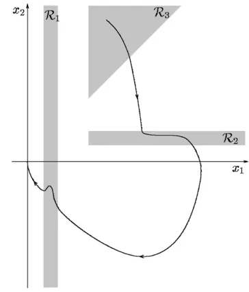
[image:6.544.303.480.91.302.2]similarities of thex-trajectories of the solutions. The state trajectories are illustrated in Figs.1and2.
Fig. 1.x-trajectory of the solution of the tuning function design.
Fig. 2. x-trajectory of the solution of the adaptive backstepping design.
Lemma 3. (i)For both designs for any design con-stants thex-trajectories start inR3,leave it through
the x1=x2 line, enter R2 through the x2 = 2 line,
leave it through the x2 = 1 line, enter R1 with
[image:6.544.297.479.344.557.2]converge to the origin,not returning to any of these three regions.
(ii) If = 2, then ˆ1 = 0, ˆ = ˆ2 and the
x-trajectories are the same for the two designs until they reachR1.
(iii)If ¡1 and is small enough,then |−ˆ|
¡8=M when the trajectory of the tuning function design entersR1.
(iv)If ¡1and2is small enough,thenˆ1=0and
|−ˆ2|¡8=M when the trajectory of the adaptive
backstepping design entersR1.
Proof. Look at the two systems outsideR1. The
tun-ing function design is ˙
x1=x2;
˙
x2=u+2; x(0) =x0;
˙ˆ
=(x2+x1)2; ˆ(0) = 0;
y=x1;
u=−4x2−4x1−2;ˆ (27)
and the adaptive backstepping design is ˙
x1=x2;
˙
x2=u+2; x(0) =x0;
˙ˆ
1= 0; ˆ1(0) = 0;
˙ˆ
2=2(x2+x1)2; ˆ2(0) = 0;
y=x1;
u=−4x2−4x1−2ˆ2; (28)
(ii) is an immediate consequence of these forms. (i) Consider (27). The x-trajectories start in
R3 because x0∈R3 and they leave R3, because
limt→∞y(t) = 0 along the solution (and sincey=x1
and R3 does not intersect the line x1 = 0). In
R3;x˙1=x2¿0. Also, ˙ˆ60 and ˆ(0) = 0;so ˆ60.
Since260 and¿0, this implies thatu60 and as
a consequence ˙x260 inR3. So the x-trajectory has
decreasingx2-coordinate and increasingx1-coordinate
in R3, so it leaves this region through the x1 =x2
line with x1¿ x1(0) = 20. For x2¿0; x˙1¿0, so
until x2¿0 (i.e. until the x-trajectory reaches the
x2 = 0 line) the x1-coordinate of the x-trajectory is
increasing. Since along the solution limt→∞x1(t)=0,
this can only happen if the x-trajectory crosses R2
as stated in (i) (since the left border of R2 is at
x1 = 9:5¡20), then reaches the x2 = 0 axis with
x1¿ x1(0) = 20. LetT be the time, whenx2(T) = 0.
Look now at the system ˙
x1=x2; x1(T) =X ¿20;
˙
x2=−4x2−4x1; x2(T) = 0; (29)
which describes the behaviour of the x-trajectory of (27) for x260; x1¿2 (i.e. after it has crossed
the x2= 0 axis and before it reaches R1). The
so-lution of this is x1(t + T) = Xe−2t(2t + 1) and
x2(t + T) = −4Xte−2t, from which we get that
˙
x2(t +T) = 4Xe−2t(2t −1). This implies that the
x2-coordinate of the trajectory is decreasing fort ¡12
and increasing for t ¿1
2. At t = 12; x1(T + 12) =
2X=e¿2, so the trajectory entersR1 att∗+T with
t∗¿1
2. Using this, and thatx2(t∗+T) =−4t∗x1(t∗+
T)=(1 + 2t∗) = −4 + 4=(1 + 2t∗), we get that
−46x2(t∗ +T)6−2, when the x-trajectory
en-tersR1. By (ii), the behaviour of the x-trajectory of
the adaptive backstepping design is the same until it reaches R1. Again, using that along the solution
limt→∞x1(t)=0, thex-trajectories leaveR1(through
thex1= 1 line). From the form of the solution of the
systems outside the supports of1 and2 it is easy
to conclude that they do not return to these supports, and that they converge to the origin.
(iii) and (iv) are equivalent by (ii), so we prove (iii). ( ˆ1=0, because ˙ˆ1=0 outsideR1.) Since ˙ˆ=0 between
R2andR1, we only have to show that|−ˆ|¡8=M
when thex-trajectory leavesR2. LetTbe the last time,
whenx2(T) =32 (thisT exists, since thex-trajectory
entersR2withx2= 2 and leaves it withx2= 1). Since
this is the last time, ˙x2(T)60. We already saw, thatx1
is increasing forx2¿0, sox1(T)¿ x1(0)=20. Hence
by the deGnition of 2; 2(x1(T); x2(T)) =Mx1(T).
Then
0¿x˙2(T) =−4x1(T)−4x2(T)−( ˆ(T)−)2
¿−8x1(T)−Mx1(T)( ˆ(T)−); (30)
from which
−ˆ(T)68=M (31)
and since ˆ is increasing inR2, the same inequality
also need to show, that ˆ(T)−68=M ifis small enough. Since ˙ˆ=(x2 +x1)2;ˆincreases in R2.
If it does not reach, we are done by (31). After it reached, ˙x26−4x1−4x2¡−4x1. But|˙ˆ|¡2Mx21
(since inR2, 0¡ x2¡ x1), so|=˙ˆx˙2|¡ Mx1L∞=2.
We now give an upper bound onx1L∞. Look at the
Lyapunov function
V=1
2x21+12(x1+x2+1ˆ)2+
1
2(−ˆ)2; (32)
which has derivative ˙V=−x2
1−3(x1+x2+1ˆ)2¡0.
This shows thatx1L∞¡2V(0)¡ -=√for some
constant -. (since we assumed that ¡1). Hence |=˙ˆx˙2|¡ -√M=2. Lett1be the time when ˆ(t1) =,
and lett2be the time when thex-trajectory leavesR2.
Since ˙x2¡0 on [t1; t2], we can conclude, that there is
t∗∈[t1; t2] such that
ˆ
(t2)−ˆ(t1)
x2(t2)−x2(t1)
=
˙ˆ
(t∗)
˙
x2(t∗)
¡
-√
M
2 ; (33)
which implies that|ˆ(t2)−ˆ(t1)|¡ -√M=2 (since
|x2(t2)−x2(t1)|¡1). If ¡162=(-2M4), then|ˆ(t2)−
|=|ˆ(t2)−ˆ(t1)|¡8=M follows, which is what we
wanted to prove.
The following lemma states the diLerence between thex-trajectories of the solutions. Under certain cir-cumstances and when and H (the height of 1),
is varied, inR1 the adaptive backstepping trajectory
remains uniformly bounded, on the other hand the tuning function design trajectory follows the curve
x2=−1(x1).
Lemma 4. (i) (Tuning function design) There are
E; 0; M0¿0, such that if ¡ 0 and M =M0,
then for all ; H ¿0 and for all t such that 16x1(t)62;|(x2+1)(t)|¡ E.
(ii) (Adaptive backstepping design) There are
D; 0; M0¿0,such that if1; 2¡ 0andM=M0,
then for all ; H ¿0 and for all t such that 16x1(t)62;|x2(t)|¡ D.
Proof. (i) Let T be the Grst time, when the tun-ing function system reaches R1. By Lemma 3,
−46x2(T)6 − 2 and clearly x1(T) = 2.
Con-sider Grst the following modiGed system with initial
condition as above: ˙
x1=x2+1; x1(T) = 2;
˙
x2=−4x2−4x1−41−1(x2+1);
−46x2(T) =X6−2: (34)
Equivalently, withw1=x1; w2=x2+1we have
˙
w1=w2; w1(T) = 2;
˙
w2=−4w2−4w1;
−46w2(T) =W6−2: (35)
The (w1; w2)-solution of this system depends
contin-uously onW, and since the possibleW values form a compact set, there areE ¿0 andt0such thatw1(T+
t0)¡1 (i.e. the w-trajectory, which approaches the
origin since
0 1
−4 −4
is Hurwitz, leaves R1 for any possible W within
t0 time), and for all T6t6t0 +T; |x2 +1|=
|w2(t)|¡ E. If and |ˆ(T)−| are small enough,
then the right hand side of the tuning function sys-tem and (34) are close to each other in anL∞sense,
so applying Theorem 37 of Appendix C4 of [9] on [T; T +t0] (on the continuous dependence of the
so-lution of a diLerential equation on the right-hand side of the equation) gives that the solutions of the two systems are arbitrarily close on [T; T +t0]. By (iii)
of Lemma3, we know that with small enoughand large enoughM;|ˆ(T)−|is arbitrarily small. Hence we can conclude that for small enough and large enoughM; |x2+1|6E inR1, which is what we
wanted to prove.
(ii) Let nowT be the time, when the adaptive back-stepping system reaches R1. Using Theorem 37 of
[9] again, we only have to show that for someD ¿0 andt0¿0; x1(t0)¡1 and|x2(t)|¡ Dfor allT6t6
T +t0are satisGed for the solution of the system
˙
x1=x2+1; x1(T) = 2;
˙
x2=−4x2−4x1−1;
Using the Lyapunov functionV=x2
1=2 + (x1+x2)2=2,
which has derivative ˙V=−x2
1−3(x1+x2)2we can
con-clude thatx1→0, hence thex-trajectory of this
sys-tem indeed leavesR1for anyX. It also givest0¿0, a
bound on the time needed to crossR1. We show that
(x2+1)(t)¡0 for allt¿T. Indeed, this is true for
t=T. Suppose for a contradiction thatt∗ is the Grst
time such that (x2+1)(t∗) = 0. Then ˙x1(t∗) = 0,
hence the velocity vector of the x-trajectory of the solution at timet∗ is vertical. Since the x-trajectory
starts (at timeT) below the graph ofx2=−1, when
it reaches it the Grst time, the velocity vector can-not point down. Hence ˙x2(t∗)¿0. On the other hand
˙
x2(t∗) =−3x2(t∗)−4x1(t∗)−(x2 +1)(t∗)¡0.
This contradiction show thatx2+1 ¡0. Now we
compute dx2=dx1as follows:
dx2
dx1 =
−4x2−4x1−1
x2+1
=−4 + 3x1−4x1
2+1 ¿−4 (37)
and claimx2(t)62 for allt ¿ T with 16x1(t)62.
Indeed, if not, then for somet∗¿ T with 16x1(t∗) 62,x2(t∗)¿2. Then for someT ¡ t∗∗¡ t∗
dx2
dx1(t
∗∗) =x2(T)−x2(t∗)
x1(T)−x1(t∗)¡
−2−2
2−x1(t∗)¡−4;
which is a contradiction. On the other handx2(t)¿
−4, since thex-trajectory starts (at timeT) above this line, hence ift∗ is the Grst time when x
2(t∗) =−4,
then ˙x2(t∗)60. But ˙x2(t∗) =−4x2(t∗)−4x1(t∗)−
1=16−4x1(t∗)−1 ¿8, which is a contradiction.
Putting this together we get −4¡ x2¡−2 in R2,
henceD= 4 completes the proof.
Lemma 5. For the0; M0; E; Dof Lemma4,for any
&1; &2¿0, G ¿ Dand for small enough 'there are
K; ; Hsuch thatH−E ¿ Gand ifTF(;10)is an
'-suboptimal tuning function controller designed to regulate the output toyr= 10,then ¡ 0.
Proof. We show Grst that since sup{x1: (x1; x2)∈R1}
= 2¡10, if the controller is designed to regulate the output toyr= 10, then thex-trajectory of the solution
does not enter R1. This follows easily from similar
arguments we used to prove Lemma3, noting that the
only signiGcant diLerence the yr term makes is that
after thex-trajectory enters thex260; x1¿0
quater-plane at time T, it satisGes the diLerential equation system
˙
x1=x2; x1(T) =X ¿20;
˙
x2=−4x2−4(x1−10); x2(T) = 0; (38)
which has solutionx1(t+T)=Xe−2t(2t+1)+10¿10
andx2(t+T) =−4Xte−2t. We set1 ≡0. The
con-sequence of the previous argument is that this change would not eLect the solution, and hence the cost.
For a Gxed constant3andK letK = 1=K2; K= 1=K; MK=M0; HK=3K, and use the notationyK=x1K,
xK
2;ˆK anduK for the x-trajectory and control u of
the closed loopsystem (; TF(K;10)). If3is large enough, then KHK−E=3−E ¿ G ¿ D. First we show that there is a constant, such that ifK is large enough, then
P(; TF(K;10)) =yKL∞+&1x2L∞
+&2uKL∞¡ : (39)
The Lyapunov function
V =1
2(x1−10)2+21(x1−10 +x2)2
+21(−ˆ)2 (40)
has derivative ˙V=−(x1−10)2−3(x1−10+x2)2¡0
along the solution, hence for everyt¿0; |xK
1(t)−10|
62V(0); |(x1(t) − 10 + x2(t)|62V(0) and
( −ˆ(t))262V(0) = 2V(0)=K2. Since V(0) is
constant, this means that there is a constant1, such
that for every t¿0; |xK
1(t)|¡ 1; |ˆK(t)|¡ 1=K.
Since xK
2(t)6x2K(0), and for xK2 ¡0 we know
the explicit form of the solution: |xK
2(t + T)| =
4Xte−2t¡41te−2t, there is a constant2, such that |xK
2(t)|¡ 2. By the choice of 2 there is a constant
3 such that |2|6MK|xK1|¡ 3K. Since 1 ≡ 0,
uK(t) = (−4xK
2 −4(x1K−10)−2ˆ)(t), hence|uK|is
indeed bounded by a constant, so there is a constant
satisfying (39).
To complete the proof, we now show that there is aK such that for any ¿ 0, if u is the control of
then&2uL∞(R3)¿ . This shows that for this setup
the choice ¿ 0 does not give'-suboptimal tuning
function controller for any small enough', which is what we wanted to show. LettK be the time when the x-trajectory of the solution leaves the region
R
3={(x1; x2):x2−1¿x1¿10:5}, where2=−K.
Suppose that there is at0¿0 such that for allK∗¿0
there isK ¿ K∗such thatt
K¿ t0. InR3; x1; x2¿10
and2≡ −K, hence ˙ˆ=(x2+x1)2¡−200K.
Therefore ˆ(tK)¡ − 20t00K, hence |u(tK)| = 4xK
2 + 4(x1K−10) +2 ¿ˆ 20t00K2¿ =&2 ifK is
large enough. If on other hand limK→∞tK= 0, then limK→∞|x1(tK)−x1(0)|= 0, since|x˙1|=|x2|6x2(0)
on R
3. Since x1(tK) =x2(tK)−1, this means, that limK→∞|x2(tK)−x2(0)|=x2(0)−x1(0)−1¿0, hence
limK→∞(supt∈[0;tK]|x˙2|)=∞. But onR3;x˙2=u+K2,
and|K2|=1, this means that limK→∞(sup|u|)=∞,
which completes the proof.
Proof of Theorem 2. Let [a; b] = [0;10]. The claim that if AB(1; 2;10) is an '-suboptimal adaptive
backstepping controller, then for =2; TF(;10)
is an'-suboptimal tuning function controller (and that they have the same costs) follows from (ii) of Lemma
3, and the fact that in this case thex-trajectories do not reachR1. According to Lemma5, for any&1; &2¿0
there is a system, such that for small enough 'if
TF(;10) is an '-suboptimal tuning function
con-troller, then ¡ 0. In this case we can apply Lemma
4for the designs (; TF(;0)) and (; AB(; ;0))
to get a signiGcant diLerence between xTF
2 L∞ and
xAB
2 L∞. The solutions for the two designs agree
un-til they reachR1, letT be the time, when they arrive
there. Then
xAB
1 L∞[0;T]+&1xAB2 L∞[0;T]+&2uABL∞[0;T]
=xTF
1 L∞[0;T]+&1xTF2 L∞[0;T]
+&2uTFL∞[0;T]: (41)
Moreover,xTF
2 L∞(R1)¿ H−E ¿ Gis much bigger
than these if3of the construction of Lemma5is large enough, sinceG ¿ D can be chosen arbitrarily. This means, that for large enough3it is enough to establish that the adaptive backstepping cost is less than the
tuning function cost inR1.
xAB
1 L∞(R1)=xTF1 L∞(R1)= 2; (42)
xTF
2 L∞(R1)¿ H−E ¿ G ¿ D
¿xAB
2 L∞(R1): (43)
We show now that there is a constant, such that xTF
2 L∞(R1)¿ uABL∞(R1): (44)
This is enough, since then by appropriately choosing
&1and&2will result
&1xTF2 L∞(R1)¿ &1xAB2 L∞(R1)
+&2uABL∞(R1); (45)
which is enough to conclude that the tuning function cost is bigger. To prove (44) look at the control of the adaptive backstepping system inR1. According to
Lemma4, there is'∗¿0 such thatˆ2−¡ '∗and
ˆ1¡ '∗inR1. Then
|uAB|64|xAB
2 |+ 4|xAB1 |+ 3|1ˆ1|+|1ˆ2|
+|
1ˆ1x2AB|+|1ˆ11ˆ2|+|111xAB1 |
64D+ 8 + 3H'∗+H(+'∗) +|
1|D'∗
+|
1|H(+'∗)'∗+ 2H21
6H; (46)
for some ¿0 if H and are large enough and
1 is small enough. This completes the proof, since
xTF
2 L∞(R1)¿ H=2.
5. Summary
By means of two examples, we have shown that overparameterisation can be beneGcial in adaptive control. This fully motivates a more general study into the whole question of when and when not to overpa-rameterise, although as noted in the Introduction, this is likely to be a challenging task.
References
[2] M. French, An analytical comparison between the weighted LQ performance of a robust and an adaptive backstepping design, IEEE Trans. Automat. Control 47 (4) (2002) 670–675. [3] M. French, Cs. SzepesvXari, E. Rogers, Uncertainty,
per-formance and model dependency in approximate adaptive non-linear control, IEEE Trans. Automat. Control 45 (2) (2000) 353–358.
[4] M. French, Cs. SzepesvXari, E. Rogers, An asymptotic scaling analysis of LQ performance for an approximate adaptive control design, Math. Control, Signals Systems 15 (2) (2002) 145–176.
[5] Z.-P. Jiang, I. Mareels, Robust nonlinear integral control, IEEE Trans. Automat. Control 15 (8) (2001) 1336–1342.
[6] I. Kanellakopoulos, P.V. KokotoviXc, A.S. Morse, Systematic design of adaptive controllers for feedback linearisable systems, IEEE Trans. Automat. Control 36 (11) (1991) 1241–1253.
[7] M. KrstiXc, I. Kanellakopoulos, P.V. KokotoviXc, Adaptive nonlinear control without overparameterization, Systems and Control Letters 19 (1992) 177–185.
[8] M. KrstiXc, I. Kanellakopoulos, P.V. KokotoviXc, Nonlinear and Adaptive Control Design, 1st Edition, Wiley, New York, 1995.