A Class of Trigonometric B´ezier Basis Functions with Six Shape Parameters over Triangular Domain

(1)

A Class of Trigonometric B´ezier Basis Functions

with Six Shape Parameters over Triangular Domain

Lianyun Peng and Yuanpeng Zhu

Abstract—In this work, a class of trigonometric Bézier basis functions over triangular domain with six shape parameters is constructed. With the new developed basis functions, a kind of trigonometric Bézier patch over triangular domain is given. For the fixed control nets, the shape of the resulting patch can be still modified flexibly by using the six shape parameters. A de Casteljau-type algorithm is proposed for computing the patch stably and efficiently. And the sufficient conditions for joining two trigonometric Bézier patches with G1 continuous smoothness are deduced. Several numerical examples are given and the results show that the new class of trigonometric Bézier basis functions is suited for surface modeling.

Index Terms—Trigonometric B´ezier basis, triangular domain, triangular patch, shape parameter, de Casteljau-type algorithm

I. INTRODUCTION

T

RIGONOMETRIC polynomials have been widely de-veloped for constructing spline curves and surfaces within computer-aided geometric design (CAGD), and the splines are widely applied in many fields of engineering, such as the data fitting presented in [1], principal components analysis in [2], data approximation to signal restoration in [3] and so on.

In [4], the recurrence relation for a kind of trigonometric B-splines was given. In [5], a class of trigonometric Lagrange and Bernstein polynomials was developed. In [6], [7], [8], [9], [10], some quadratic trigonometric B-splines possessing local shape parameters were proposed. In [11], a family of cubic trigonometric Bézier (T-Bézier, for short) basis with a shape parameter was shown. In [12], a new cubic T-Bézier basis with two shape parameters was further extended. In [13], [14], shape features of the T-Bézier curves were analyzed with the envelop and topological mapping theory. There are some recent papers concerning representation of curves using trigonometric spline with shape parameters; see for example [15], [16] and [17], and the references quoted therein. In [16], a class of rational cubic/quadratic interpolation spline with three local free parameters was constructed. In [17], a kind of C1 rational cubic/linear trigonometric interpolation spline possessing two local pa-rameters was presented. For the univariate splines, by using the classical tensor product method, we can easily obtain bi-variate splines with shape parameters through these new basis functions. However, we cannot get basis functions over triangular domain with shape parameters by the method of tensor product. For some practical surfaces modeling, basis functions over triangular domain are important.

Recently, some new basis functions over triangular domain have been proposed; see [18], [19], [20], [21], [22], [23],

Manuscript received May 03, 2019; revised September 16, 2019. Lianyun Peng, Yuanpeng Zhu are with School of Mathematics, South China University of Technology, Guangzhou510640, PR China (e-mail: [email protected]; [email protected]).

[24], [25], [26] and the references quoted therein. In [18], a class of Bernstein-Bézier basis functions with a shape parameter over triangular domain was given. In [19], a kind of Bernstein-like trigonometric basis functions with a shape parameter over triangular domain was given, which was an extension of the third-order p-Bézier basis given in [27]. In [20], a new Bézier-like basis over triangular domain with a shape parameter was constructed, which can be used to construct some surfaces with three boundaries of ellipse arcs. In [21], a set of triangular Bézier surfaces with shape parameters was presented. In [22], a class of triangular Bernstein-Bézier-like surface with a shape parameter was given. In [23], a kind of Bernstein-Bézier basis functions over triangular domain possessing three exponential shape parameters was constructed, which included the cubic tri-angular Bernstein-Bézier basis together with Said-Ball basis as special cases. Recently, in [24], four new trigonometric Bernstein-like basis functions with two exponential shape parameters are constructed. In [25], a class of trigonometric polynomial basis functions over triangular domain with three shape parameters is proposed. In [26], a practical method of generating triangular polynomial surface in triangular domain is presented, and the basic functions of triangular polynomial surface with three shape parameters over triangular domain are given.

The purpose of this paper is to present a new class of trigonometric B´ezier basis functions over triangular domain, which has six shape parameters and is useful for generating triangular B´ezier patch. It improves on the existing schemes in some ways:

1) The basis functions mentioned in [24], have two pa-rameters. Other basis functions mentioned in [25], [26], have only three parameters. And our basis functions have six parameters in the corresponding triangular B´ezier patch, which have a predictable adjusting role on the patch;

2) The new class of basis functions is a summary of the existing basis functions, include some special cases given in [24], [25], [26], [28], therefore it is more general in method.

The rest of this paper is organized as follows. Section II gives the construction and properties of the trigonometric Bézier basis functions over triangular domain. In Section III, the definition and properties of the trigonometric Bézier patch over triangular domain with six shape parameters are shown. A practical de Casteljau-type algorithm for com-puting the proposed trigonometric Bézier patch over the triangular domain is developed. Conclusions are given in Section IV.

IAENG International Journal of Applied Mathematics, 49:4, IJAM_49_4_30

(2)

II. A T-B ´EZIER CURVE WITH SHAPE PARAMETERS OVER A TRIANGULAR DOMAIN

A. Definition of the new base function

Definition 1: For any α, β, γ ∈ [1,+∞), λ ∈ [−α,1], µ∈[−β,1],η∈[−γ,1], the following ten functions

B33,0,0= (1−cosu)α(1−λcosu), B3

0,3,0= (1−cosv)β(1−µcosv), B3

0,0,3= (1−cosw)γ(1−ηcosw), B23,1,0= coswsinv(1−cosu)

×[1+cosu₋(1₋cosu)α−1₍₁₋_λ_cos_u₎

cosu

] ,

B3

2,0,1= cosvsinw(1−cosu)

×[1+cosu−(1−cosu)α−1(1−λcosu) cosu

] ,

B3

1,2,0= coswsinu(1−cosv)

×[1+cosv−(1−cosv)β−1(1−µcosv) cosv

] ,

B3

0,2,1= cosusinw(1−cosv)

×[1+cosv−(1−cosv)β−1₍₁₋_µ_cos_v₎

cosv

] ,

B3

1,0,2= cosvsinu(1−cosw)

×[1+cosw₋(1₋cosw)γ−1₍₁₋_η_cos_w₎

cosw

] ,

B03,1,2= cosusinv(1−cosw)

×[1+cosw₋(1₋cosw)γ−1₍₁₋_η_cos_w₎

cosw

] ,

B3

1,1,1= 1−(B33,0,0+B30,3,0+B03,0,3+B23,1,0 +B3

2,0,1+B13,2,0+B03,2,1+B31,0,2+B03,1,2), (1) are defined as trigonometric B´ezier basis functions with six shape parameters over the triangular domain D = {

(u, v, w)u+v+w=π₂π/2, u≥0, v≥0, w≥0}.

Remark1: When one of the three variableswis taken as zero, the ten trigonometric B´ezier basis functionsB3_i,j,k(i+ j+k= 3;i, j, k≥0) will degenerate to the following four cubic trigonometric B´ezier-Type (TB-type for short) basis functions (noticev=π/2−u) with four shape parametersα, β,λandµgiven in [28]

      

T0(t) = (1−sint)α(1−λsint),

T1(t) = 1−sin2t−(1−sint)α(1−λsint), T2(t) = 1−cos2t−(1−cost)β(1−µcost), T3(t) = (1−cost)β(1−µcost).

Remark2: Here, we give some hints on how to construct the ten trigonometric B´ezier basis functions over triangular domain. Our starting point is to extend the four univariate trigonometric basis functions given in [28] to ten multi-variable basis functions over triangular domain such that the ten multi-variable basis functions can degenerate to the four univariate trigonometric like basis functions when one of the three variables is taken as zero and form a partition of unity. With these thoughts in mind, it is easy to construct the function B3

3,0,0(u, v, w;α, β, γ;λ, µ, η) and symmetrically we can obtain the formulas ofB3

0,3,0(u, v, w;α, β, γ;λ, µ, η) and B3

0,0,3(u, v, w;α, β, γ;λ, µ, η). Next, we shall con-struct the two functions B3

2,1,0(u, v, w;α, β, γ;λ, µ, η) and B3₂_,₀_,₁(u, v, w;α, β, γ;λ, µ, η)at the same time. As is shown in Remark 1, when one of the three variables w is taken as zero, the function B23,1,0(u, v, w;α, β, γ;λ, µ, η) should degenerate to the bivariate functionT2(u;α;λ)(noticev= π/2−u ) and the function B23,0,1(u, v, w;α, β, γ;λ, µ, η)

should vanish. Analogously, when one of the three vari-ables v is taken as zero, we can get a similar conclusion that the functionB3

2,1,0(u, v, w;α, β, γ;λ, µ, η)should van-ish while the functionB3

2,0,1(u, v, w;α, β, γ;λ, µ, η)should degenerate to the bivariate function T2(u;α;λ) (notice w = π/2 − u ). These give us a hint that the func-tion T2(u;α;λ) should be divided into two multi-variable functions and B₂3_,₁_,₀(u, v, w;α, β, γ;λ, µ, η) is reasonable to possess the factor of coswsinv. From these and notice that cosu = coswsinv + sinwcosv for u+v +w = π/2, we can immediately divide T2(u;α;λ) into a pair of multi-variable function B23,1,0(u, v, w;α, β, γ;λ, µ, η) and B3

2,0,1(u, v, w;α, β, γ;λ, µ, η). Similarly, we can ob-tain the four functions B3

1,2,0(u, v, w), B03,2,1(u, v, w), B3

1,0,2(u, v, w)andB30,1,2(u, v, w). Finally, considering the property of partition of unity, it is natural to obtain the formula ofB3

1,1,1(u, v, w;α, β, γ;λ, µ, η).

Whenu=π/2orv=π/2orw=π/2, the trigonometric B´ezier basis functionsB_i,j,k3 (i+j+k= 3;i, j, k≥0) degen-erate toTi(i= 0,1,2,3). SoB3

i,j,k(i+j+k= 3;i, j, k≥0) can be seen as a generalization of Ti(i = 0,1,2,3) over triangular domain given in [28].

Remark3: Forλ =µ =η = 0, the ten basis functions given in (1) will return to the ten basis functions with three exponential shape parameters given in [24]. And for anyα= β=γ= 2, it is easy to check that the ten functions (1) will return to the ten basis functions with three shape parameter given in [25]. Moreover, for any α=β =γ= 1, it is easy to check that the ten functions (1) will return to the ten basis functions with three shape parameters given in [26].

Before further discussion, we provide the following lem-ma, which is useful in the following discussion and proved in [25].

Lemma1: Foru+v+w= π₂, we have

1−(sin2u+ sin2v+ sin2w)= 2 sinusinvsinw. (2)

B. Properties of the new basis function

From the definition of the basis functions with shape parameters over the triangular domain, we can obtain the following important properties of the basis functions.

Theorem1: The basis functions with shape parameters (1) have the following properties:

(A) Nonnegativity:B3

i,j,k(i+j+k= 3;i, j, k≥0)≥0. (B) Partition of unity:∑B_i,j,k3 (i+j+k= 3;i, j, k≥0)=1. (C) Symmetry: For alli+j+k= 3, i, j, k≥0, we have

B_i,j,k3 (u, v, w;α, β, γ;λ, µ, η) =B3

j,i,k(u, v, w;α, β, γ;λ, µ, η), =B3

j,k,i(u, v, w;α, β, γ;λ, µ, η), =B3

i,k,j(u, v, w;α, β, γ;λ, µ, η), =B3

k,i,j(u, v, w;α, β, γ;λ, µ, η), =B_k,j,i3 (u, v, w;α, β, γ;λ, µ, η).

(D) Boundary properties: When one of the three variables u,v,w is set to be π/2, then the basis functions with shape parametersB3

i,j,k(i+j+k= 3;i, j, k≥0) will degenerate to Ti(i= 0,1,2,3) given in Remark 1.

(E) Linear independence: {

B3

i,j,k(i+j+k= 3;i, j, k≥0) }

are linearly independent.

IAENG International Journal of Applied Mathematics, 49:4, IJAM_49_4_30

(3)

Proof: We shall prove (A) and (E). The remaining prop-erties can be proved easily.

(A) Apparently, for any α, β, γ ∈ [1,+∞), λ ∈ [−α,1], µ ∈ [−β,1], η ∈ [−γ,1], we have B3_i,j,k(i+j+k = 3;i, j, k ≥ 0;i, j, k ̸= 1) ≥ 0. Furthermore, for B3

1,1,1, using Lemma 1, we have

B3

1,1,1= 1− ∑

i+j+k=3 i·j·k̸=1

B3 i,j,k

= 1−(sin2u+ sin2v+ sin2w) = 2 sinusinvsinw≥0.

(E) For any α, β, γ ∈ [1,+∞), λ ∈ [−α,1], µ ∈ [−β,1],ζi,j,k∈R,(i+j+k= 3, i, j, k∈N), we consider a linear combination

∑

i+j+k=3 i,j,k∈N

ζi,j,kB_i,j,k3 = 0.

Letw= 0, we have

3 ∑

i=0

ζi,3−i,0Ti(t) = 0. (3)

Differentiating with respect to the variablevon both sides, we have

3 ∑

i=0

ζi,3−i,0Ti′(t) = 0. (4)

Forv = 0, from (3) and (4), we get the following linear system of equations with respect toζ0,3,0 andζ1,2,0

{

ζ0,3,0= 0,

(α+λ)(ζ1,2,0−ζ0,3,0) = 0.

[image:3.595.281.549.51.578.2]

Thus, we haveζ0,3,0 =ζ1,2,0 = 0. For t =π/2from (3) and (4), we haveζ3,0,0 =ζ2,1,0= 0. Similarly,ζi,0,3−i = ζ0,i,3−i = 0 for i = 0,1,2,3. Finally, ζ1,1,1 = 0. These imply the theorem.

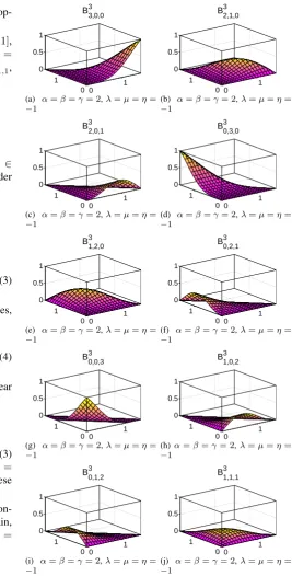
Fig. 1 shows the trigonometric B´ezier basis function-s B3

i,j,k(i+j+k= 3;i, j, k ≥0) over triangular domain, where the six shape parameters are α = β = γ = 2, λ = µ=η=−1.

III. ATRIANGULARB ´EZIER PATCH WITH SIX SHAPE PARAMETERS OVER TRIANGULAR DOMAIN

A. Definition and properties of triangular B´ezier patches

Definition 2: For any α, β, γ ∈ [1,+∞), λ ∈ [−α,1], µ ∈ [−β,1], η ∈ [−γ,1], over triangular domain D ={(u, v, w)u+v+w=π₂, u≥0, v≥0, w≥0}, the control points Pi,j,k ∈ R3_, _i₊_j₊_k _{= 3}_, _i _≥ ₀_, _j _≥ ₀_, k≥0, we call the patch

R(u, v, w) = ∑ i+j+k=3

B_i,j,k3 Pi,j,k (5)

be the triangular B´ezier patch with six shape parameters over triangular domain.

According to the properties of the basis functions with shape parameters given in Theorem 1, some properties of the corresponding triangular B´ezier patch given in (5) can be obtained as follows:

0 1 0

1 0 0.5 1

B 3,0,0 3

(a) α=β=γ= 2,λ=µ=η=

−1

0 1 0

1 0 0.5 1

B 2,1,0 3

(b) α=β=γ= 2,λ=µ=η=

−1

0 1 0

1 0 0.5 1

B_2,0,13

(c) α=β=γ= 2,λ=µ=η=

−1

0 1 0

1 0 0.5 1

B_0,3,03

(d) α=β=γ= 2,λ=µ=η=

−1

0 1 0

1 0 0.5 1

B 1,2,0 3

(e) α=β=γ= 2,λ=µ=η=

−1

0 1 0

1 0 0.5 1

B 0,2,1 3

(f) α=β=γ= 2,λ=µ=η=

−1

0 1 0

1 0 0.5 1

B 0,0,3 3

(g) α=β=γ= 2,λ=µ=η=

−1

0 1 0

1 0 0.5 1

B 1,0,2 3

(h)α=β=γ= 2,λ=µ=η=

−1

0 1 0

1 0 0.5 1

B 0,1,2 3

(i) α=β=γ= 2,λ=µ=η=

−1

0 1 0

1 0 0.5 1

B 1,1,1 3

(j) α=β=γ= 2,λ=µ=η=

−1

Fig. 1. The plots of trigonometric B´ezier basis functions over trigonometric domain.

(A) Affine invariance and convex hull property. Since basis functions with shape parameters (1) have the properties of the partition of unity and nonnegativity, these imply that the corresponding triangular B´ezier patch (5) has affine invariance and convex hull property.

(B) End point interpolation property. Through direct com-putation, we can get that R(π/2,0,0) = P3,0,0, R(0, π/2,0) =P0,3,0,R(0,0, π/2) =P0,0,3.

These indicate that the triangular B´ezier patch interpo-lates at the three end points.

(C) End point tangent property. Letw=π/2−u−v, we

IAENG International Journal of Applied Mathematics, 49:4, IJAM_49_4_30

(4)

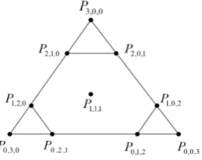
Fig. 2. Schematic diagram of B´ezier patch control points and control grids over triangular domain.

have

∂R(u,v,w) ∂u

(π/2,0,0)= (λ+α)P3,0,0−(λ+ 1)P2,0,1 + (1−α)P1,1,1,

∂R(u,v,w) ∂v

(π/2,0,0)

= (λ+ 1) (P2,1,0−P2,0,1),

∂R(u,v,w) ∂u

(0,π/2,0)

= (µ+ 1) (P1,2,0−P0,2,1),

∂R(u,v,w) ∂v

(0,π/2,0)= (µ+β)P0,3,0−(µ+ 1)P0,2,1 + (1−β)P1,1,1,

∂R(u,v,w) ∂u

(0,0,π/2)= (η+ 1)P1,0,2−(η+γ)P0,0,3 + (γ−1)P1,1,1,

∂R(u,v,w) ∂v

(0,0,π/2)

= (η+ 1)P0,1,2−(η+γ)P0,0,3

+ (γ−1)P1,1,1.

These indicate that the tangent plane at the three end points (π/2,0,0), (0, π/2,0), (0,0, π/2) are the three planes spanned by the control points P3,0,0, P2,1,0, P2,0,1, P0,3,0, P1,2,0, P0,2,1, P0,0,3, P1,0,2, P0,1,2 and P1,1,1 respectively.

(D) Boundary property. For w = 0, R(t, s, w) is just the following cubic T-B´ezier curve given in [28] with four shape parametersα,β,λandµ.

R(u, π/2−u,0)= 3 ∑

i=0

Pi,3−i,0Ti(u;λ, µ) (6)

Similarly, R(0, v, π/2−v) and R(π/2−w,0, w) are also T-Bézier curve with shape parameters β, γ, µ, η and α, γ, λ,η respectively. Forα=β = 1,λ=µ= 0, the T-Bézier curve (6) can represent exactly elliptic; For α = β = 1, λ = µ = 1, b−a>0, the T-Bézier curve (6) can represent exactly parabola arcs; For α= β = 2, λ = µ = 0, the T-Bézier curve (6) represent a quarter of elliptic arc; For α=β = 2, λ= µ= 2, b −a>0, the T-Bézier curve (6) represent a segment of the parabola; see [28]. These imply that the three boundaries of trigonometric Bézier patch (5) can be arcs of ellipse or parabola, respectively.

(E) Shape adjustable property. The control points of the trigonometric B´ezier patch are P(3,0,0) = (0,0,0), P(0,3,0) = (−2,−2,0), P(0,0,3) = (2,−2,0), P(2,1,0) = (−0.5,−0.5,1), P(2,0,1) = (−0.5,0.5,1), P(1,2,0) =

(−1.5,−1.5,1), P(1,0,2) = (1.5,−1.5,1), P(0,2,1) = (−1,−2,1), P(0,1,2) = (1,−2,1), P(1,1,1) = (0,−1.2,1.5). Fig. 2 shows the schematic diagram of Bézier patch control points and control grids over triangular domain. Without changing the control points, we can adjust the shape of the obtained trigonometric Bézier patch conveniently using the six shape parameters λ, µ, η, α, β and γ. As the six shape parameters increase at the same time, the trigonometric Bézier patch will be made close to the control net. From the boundary property of the trigonometric Bézier patch, we can see that the six shape parametersλ, µ,η, α,β andγ have nothing to do with the boundary curvesR(0, v, w),R(u,0, w)and R(u, v,0)respectively. It is equivalent that changing the value of single one shape parameter, one corresponding boundary curve will not change. Moreover, from (5), differentiating with respect to the shape parameter λ, we have

∂R(u,v,w) ∂λ

= (1−cosu)α_cos_u(P

1,1,1−P3,0,0) + coswsinv(1−cosu)α(P2,1,0−P1,1,1) +cosvsinw((1−cosu)α(P2,0,1−P1,1,1).

(7)

Therefore, there is no relationship between ∂R(u,v,w_∂λ ) and λ. These imply that for the fixed control points and the given value(u, v, w)∈D, changing single one shape parameter will make the corresponding point on the trigonometric B´ezier surface patch (5) move linearly in the direction given by (7). The shape parametersµ,η, α,β andγ have the similar effect on the trigonometric B´ezier surface patch.

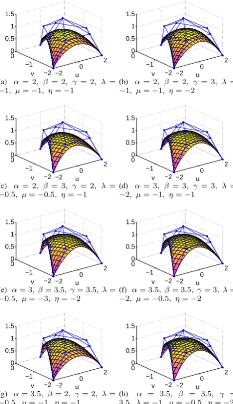
Fig. 3 shows the trigonometric B´ezier patches and the effect on the patches by altering the values of the shape parameters under the same control points.

B. De Casteljau-type Algorithm

The classical de Casteljau algorithm is a stable and effi-cient process for computing the triangular B´ezier patch. Now, we want to develop a practical de Casteljau-type algorithm for computing the proposed the triangular B´ezier surface given in (5). For this purpose, for any(u, v, w)∈D, let

f1(u, v, w) :

= sinucosw(sin

2_u_+sin2_v_+sin2_w₎

cosw(sinu+sinv)(sin2_u_+sin2_v_+sin2_w_)+sin_w_(sin2_u_+sin2_v₎,

f2(u, v, w) :

= sinvcosw(sin

2_u_+sin2_v_+sin2_w₎

f3(u, v, w) :

= sinw(sin

2_u_+sin2_v₎

g1(u, v, w) := (1−cosu) (

sin2u+ sin2v+ sin2w), g2(u, v, w) := sinvcosw

(

sin2u+ sin2v+ sin2w) + sinusinvsinw,

g3(u, v, w) := cosvsinw (

sin2u+ sin2v+ sin2w) + sinusinvsinw,

IAENG International Journal of Applied Mathematics, 49:4, IJAM_49_4_30

[image:4.595.99.247.66.183.2]

(5)

−2 0

2

−2 −1 0 0 0.5 1 1.5

u v

(a) α= 2, β = 2, γ = 2, λ =

−1, µ=−1, η=−1

−2 0

2

−2 −1 00 0.5 1 1.5

u v

(b) α= 2, β = 2, γ = 3, λ=

−1, µ=−1, η=−2

−2 0

2

−2 −1 0 0 0.5 1 1.5

u v

(c) α= 2, β = 3, γ = 2, λ =

−0.5, µ=−0.5, η=−1

−2 0

2

−2 −1 00 0.5 1 1.5

u v

(d) α= 3, β = 3, γ = 3, λ=

−2, µ=−1, η=−1

−2 0

2

−2 −1 0 0 0.5 1 1.5

u v

(e) α= 3, β= 3.5, γ= 3.5, λ=

−0.5, µ=−3, η=−2

−2 0

2

−2 −1 00 0.5 1 1.5

u v

(f) α= 3.5, β= 3.5, γ= 3, λ=

−2, µ=−0.5, η=−2

−2 0

2

−2 −1 0 0 0.5 1 1.5

u v

(g) α= 3.5, β= 2, γ= 2, λ=

−0.5, µ=−1, η=−1

−2 0

2

−2 −1 00 0.5 1 1.5

u v

[image:5.595.49.288.58.471.2]

(h) α = 3.5, β = 3.5, γ = 3.5, λ=−1, µ=−0.5, η=−2

Fig. 3. Trigonometric B´ezier patches with different shape parameters

and

P1 2,0,0:=

(1+cosu)α−2₍₁₋_λ_cos_u₎

1+cosu P3,0,0 +[1+cosu−(1+cosu)

α−2₍₁₋_λ_cos_u₎_]_sin_v_cos_w

(1+cosu) cosu P2,1,0 +[1+cosu−(1+cosu)

α−2₍₁₋_λ_cos_u₎_]_sin_w_cos_v

(1+cosu) cosu P2,0,1, P₀1_,₂_,₀:= [1+cosv−(1+cosv)

β−2₍₁₋_µ_cos_v₎_]_sin_u_cos_w

(1+cosv) cosv P1,2,0 +(1+cosv_1+cos)β−2(1_v−µcosv)P0,3,0

+[1+cosv−(1+cosv)

β−2₍₁₋_µ_cos_v₎_]_sin_w_cos_u

(1+cosv) cosv P2,0,1, P₀1_,₀_,₂:= [1+cosw−(1+cosw)

γ−2₍₁₋_η_cos_w₎_]_sin_u_cos_v

(1+cosw) cosw P1,0,2 +[1+cosw−(1+cosw)

γ−2₍₁₋_η_cos_w₎_]_sin_v_cos_u

(1+cosw) cosw P0,1,2 +(1+cosw_1+cos)γ−2(1_w−ηcosw)P0,0,3,

P11,1,0:=f1(u, v, w)P2,1,0+f2(u, v, w)P1,2,0 +f3(u, v, w)P1,1,1,

P1

1,0,1:=f1(u, v, w)P2,0,1

+f3(u, v, w)P1,1,1+f2(u, v, w)P1,0,2, P1

0,1,1:=f3(u, v, w)P1,1,1+f1(u, v, w)P0,2,1 +f2(u, v, w)P0,1,2.

Then, we can rewrite the expression of the triangular

B´ezier patch as follows:

R(u, v, w) =_sin2_u_+sin1−cos2_v2_+sinu 2_w

×[g1(u, v, w)P21,0,0+g2(u, v, w)P11,1,0 +g3(u, v, w)P11,0,1

]

+ 1−cos2v sin2_u_+sin2_v_+sin2_w

]

+_sin2_u1_+sin−cos2_v2_+sinw 2_w

] .

(8)

Furthermore, by setting

P₁2_,₀_,₀:=g1(u, v, w)P21,0,0+g2(u, v, w)P11,1,0 +g3(u, v, w)P11,0,1,

P2

0,1,0:=g2(v, u, w)P11,1,0+g1(v, u, w)P01,2,0 +g3(v, u, w)P01,1,1,

P2

0,1,0:=g3(v, u, w)P11,0,1+g2(v, u, w)P01,1,1 +g1(v, u, w)P01,0,2,

we have

R(u, v, w) =_sin2_u_+sin1−cos2_v2_+sinu 2_wP

2 1,0,0 + 1−cos2v

sin2_u_+sin2_v_+sin2_wP

2 0,1,0 +_sin2_u_+sin1−cos2_v2_+sinw 2_wP02,0,1 :=P3

0,0,0.

(9)

Foru+v+w=π/2, it is easy to check thatf1(u, v, w) + f2(u, v, w) +f3(u, v, w) = 1andg1(u, v, w) +g2(u, v, w) + g3(u, v, w) = 1 (by using Lemma 1). Thus Eqs. (8) and (9) indicate a de casteljau-type algorithm for computing the proposed triangular B´ezier patch given in (5).

C. Join two triangular B´ezier surfaces

In practical surface construction, we often need to join several patches together to generate surfaces that are too complex to handle with a single patch. During the join of the triangular B´ezier patches, we need to control the smoothness of the connecting surface. Let two triangular B´ezier patches be

R1(u, v, w) = ∑

i+j+k=3

B_i,j,k3 Pi,j,k,

and

R2(u, v, w) = ∑

i+j+k=3

B_i,j,k3 Qi,j,k.

Apparently, if the control points satisfy

P0,j,k=Q0,j,k, j, k∈N, j+k= 3, (10)

the two patches join along a common boundary curve: R1(0, v, w) =R2(0, v, w), v +w = π/2. Thus, the two patches clearly form a surface with positional continuity, or a surface withC0continuity. For the common boundary curve R1(0, v, π/2−v)differentiating with respect to v, we have

dR1(0,v,π/2−v)

dv

= sinv(1−cosv)β−1[β+µ−µ(β+ 1) cosv]

×(P0,0,3−P0,2,1) + 2 sinvcosv(P0,2,1−P0,1,2) + cosv(1−sinv)γ−1[γ+η−η(γ+ 1) sinv]

×(P0,1,2−P0,0,3).

(11)

IAENG International Journal of Applied Mathematics, 49:4, IJAM_49_4_30

(6)

ForR1(u, v, π/2−u−v)andR2(u, v, π/2−u−v), by differentiating with respect to urespectively, we get

dR1(u,v,π/2−u−v)

du

u=0

×(P0,0,3−P0,2,1) + 2 sinvcosv×(P0,2,1−P0,1,2) + cosv(1−sinv)γ−1[γ+η−η(γ+ 1) sinv]

×(P0,1,2−P0,0,3),

(12) dR2(u,v,π/2−u−v)

du

u=0

×(Q0,0,3−Q0,2,1) + 2 sinvcosv×(Q0,2,1−Q0,1,2) + cosv(1−sinv)γ−1[γ+η−η(γ+ 1) sinv]

×(Q0,1,2−Q0,0,3).

(13) The condition for smooth joining is that the vectors defined by Eq. (11) through (13) are coplanar for any value of v, see [29], which can be expressed as follows:

dR2(u,v,π/2−u−v)

du

u=0 =ϕdR1(0,v,π/2−v)

dv +φ

dR1(u,v,π/2−u−v)

du

u=0, whereϕandφboth are constants. From these, we can obtain a rule

  

Q1,2,0−Q0,2,1=ϕ(P0,3,0−P0,2,1) +φ(P1,2,0−P0,2,1), Q1,1,1−Q0,1,2=ϕ(P0,2,1−P0,1,2) +φ(P1,1,1−P0,1,2), Q1,0,2−Q0,0,3=ϕ(P0,1,2−P0,0,3) +φ(P1,0,2−P0,0,3).

(14) Summarizing the above discussion, we can conclude the following theorem.

Theorem2: Forαi, β, γ ∈[1,+∞), λ∈[−α,1], µ∈ [−β,1], η ∈ [−γ,1], i = 1,2, the surface connected R1(u, v, w) with R2(u, v, w) is continuous, if the control points satisfy the conditions (10) and (14).

[image:6.595.314.541.54.393.2]

From Theorem 2, we can see that the conditions for smooth joining two triangular Bézier patches are analogous to the conditions for joining two triangular Bernstein-Bézier patches; see [29]. However, we can adjust the shape of the obtainedG1_{continuous surface conveniently using the shape} parameters in the triangular Bézier patches.

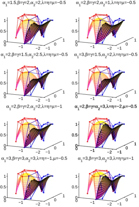
Fig. 4 shows the G1 _{continuous surface generated by} smooth joining triangular B´ezier patches with different shape parameters. The parameters take fixed valueϕ= 1andφ=

−1.

IV. CONCLUSION

The new proposed trigonometric Bézier basis functions possessing six shape parameters over triangular domain are useful for constructing surfaces in CAGD, which include some special cases given in [24], [25], [26], [28]. They have good properties such as nonnegativity, partition of unity, symmetry, linear independence and so on. With the new basis functions, we construct the trigonometric Bézier patch over triangular domain, which has some properties analogous to that of the triangular Bernstein-Bézier cubic patch. In order to computer the trigonometric Bézier patch, we propose a new practical de Casteljau-type algorithm. In the end of the paper, we show the G1 continuous smooth surfaces joining two trigonometric Bézier patches with different shape parameters, which have practical significance in the surface construction.

−1

0 1

−2 −1 0 0 0.5 1

α₁=1.5,β=γ=2,α

2=2,λ=η=µ=−0.5

−1

0 1

−2 −1 0 0 0.5 1

α₁=2,β=γ=2,α

2=1,λ=η=µ=−0.5

−1 0

1

−2 −1 0 0 0.5 1

α

1=2,β=γ=1.5,α2=2.5,λ=η=µ=−0.5

−1 0

1

−2 −1 0 0 0.5 1

α

1=3,β=γ=1.5,α2=2,λ=η=µ=−0.5

−1 0

1

−2 −1 0 0 0.5 1

α₁=2,β=γ=2,α

2=2,λ=η=µ=−1

−1 0

1

−2 −1 0 0 0.5 1

α₁=2,β=γ=α

2=3,λ=η=−2,µ=−0.5

−1 0

1

−2 −1 0 0 0.5 1

α₁=2,β=γ=α

2=3,λ=η=−2,µ=−0.5

−1 0

1

−2 −1 0 0 0.5 1

α

1=3,β=γ=3,α2=3,λ=η=−1,µ=−0.5

−1 0

1

−2 −1 0 0 0.5 1

α

[image:6.595.59.288.77.236.2]

1=3,β=γ=3,α2=3,λ=η=µ=−1

Fig. 4. G1 continuous surfaces joining two trigonometric B´ezier patches with different shape parameters

There are still some problems worthy of further study, such as the approximation power of the base functions. In practice, the extension of the given trigonometric polynomial basis over the triangular domain to higher degrees and subdivision algorithm for the proposed trigonometric polynomial patch are important considerations. These will be our future work.

ACKNOWLEDGMENT

The research is supported by the National Natural Science Foundation of China (Grant No. 61802129) and the Natural Science Foundation Guangdong Province, China (Grant No. 2018A030310381).

REFERENCES

[1] S. S. Papakonstantinou and I. C. Demetriou, “Optimality conditions for bestL1_{data fitting subject to nonnegative second differences,”}_IAENG

International Journal of Applied Mathematics, vol. 38, no.1, pp. 30-33, 2008.

[2] N. Lavado and T. Calapez, “Principal components analysis with spline optimal transformations for continuous data,” IAENG International Journal of Applied Mathematics, vol. 41, no. 4, pp. 367-375, 2011. [3] I. C. Demetriou, “An application of bestL1_{piecewise monotonic data}

approximation to signal restoration,” IAENG International Journal of Applied Mathematics, vol. 43, no. 4, pp. 226-232, 2013.

[4] T. Lyche and T. Winther, “A stable recurrence relation for trigonometric polynomial curves,”Journal of Approximation Theory 1979, pp. 266-279.

[5] G. Walz, “Trigonometric B´ezier and Stancu polynomials over intervals and triangles,”Computer Aided Geometric Design, vol. 14, no. 4, pp. 393-397, May 1997.

IAENG International Journal of Applied Mathematics, 49:4, IJAM_49_4_30

(7)

[6] X. L. Han, “Quadratic trigonometric polynomial curves with a shape parameter,”Computer Aided Geometric Design, vol. 19, no. 7, pp. 503-512, July 2002.

[7] X. Q. Wu, X. L. Han, and S. Luo, “Quadratic trigonometric polyno-mial B´ezier curves with a shape parameter,”Journal of Engineering Graphics, vol. 29, pp. 82-87, Jan. 2008.

[8] X. L. Han, “Piecewise quadratic trigonometric polynomial curves,”

Mathematics of Computation, vol. 72, no. 243, pp. 1369-1377, Mar. 2003.

[9] X. L. Han, “C2 _{quadratic trigonometric polynomial curves with local}

bias,”Journal of Computational and Applied Mathematics, vol. 180, no. 1, pp. 161-172, Aug. 2005.

[10] X. L. Han, “Quadratic trigonometric polynomial curves concerning local control,”Applied Numerical Mathematics, vol. 56, no. 1, pp. 105-115, Jan. 2006.

[11] X. L. Han, “Cubic trigonometric polynomial curves with a shape parameter,”Computer Aided Geometric Design, vol. 21, no. 6, pp. 535-548, July 2004.

[12] X. A. Han, Y. C. Ma, and X. L. Huang, “The cubic trigonometric Bzier curve with two shape parameters,”Applied Mathematics Letters, vol. 22, no. 2, pp. 226-231, Feb. 2009.

[13] X. A. Han, Y. C. Ma, and X. L. Huang, “Shape analysis of cubic trigonometric B´ezier curves with a shape parameter,”Applied Mathe-matics and Computation, vol. 217, no. 6, pp. 2527-2533, Nov. 2010. [14] R. J. Wu and G. H. Peng, “Shape analysis of planar trigonometric

B´ezier curves with two shape parameters,”International Journal of Computer Science Issues, vol. 10, no. 2, pp. 441-447, Mar. 2013. [15] X. L. Han and Y. P. Zhu, “Curve construction based on five

trigono-metric blending functions,”Bit Numerical Mathematics, vol. 52, no. 4, pp. 953-979, Dec. 2012.

[16] X. B. Qin, L. Qin, and Q. S. Xu, “C1_{positivity-preserving}

interpola-tion schemes with local free parameters,”IAENG International Journal of Computer Science, vol. 43, no. 2, pp. 219-227, 2016.

[17] X. B. Qin and Q. S. Xu, “C1 _{rational cubic/linear trigonometric}

interpolation spline with positivity-preserving property,” Engineering Letters, vol. 25, no. 2, pp. 152-159, 2017.

[18] J. Cao and G. Z. Wang, “An extension of BernsteinCB´ezier surface over the triangular domain,”Progress in Natural Science, vol. 17, no. 3, pp. 352-357, Mar. 2007.

[19] W. Q. Shen and G. Z. Wang, “Triangular domain extension of linear Bernstein-like trigonometric polynomial basis,” Journal of Zhejiang University-SCIENCE C, vol. 11, no. 5, pp. 356-364, May 2010. [20] Y. W. Wei, W. Q. Shen, and G. Z. Wang, “Triangular domain extension

of algebraicCtrigonometric B´ezier-like basis,”Applied Mathematics-A Journal of Chinese Universities, vol. 26, no. 2, pp. 151-160, June 2011. [21] L. Q. Yang and X. M. Zeng, “B´ezier curves and surfaces with shape parameters,”International Journal of Computer Mathematics, vol. 86, no. 7, pp. 1253-1263, June 2009.

[22] L. L. Yan and J. F. Liang, “An extension of the B´ezier model,”Applied Mathematics and Computation, vol. 218, no. 6, pp. 2863-2879, Nov. 2011.

[23] Y. P. Zhu and X. L. Han, “A class ofαβγ-BernsteinCB´ezier basis functions over triangular domain,”Applied Mathematics and Computa-tion, vol. 220, no. 1, pp. 446-454, Sept. 2013.

[24] Y. P. Zhu and X. L. Han, “New trigonometric basis possessing exponential shape parameters,”Journal of Computational Mathematics, vol. 33, no. 6, pp. 642-684, Nov. 2015.

[25] X. L. Han and Y. P. Zhu, “A Practical Method for Generating Trigono-metric Polynomial Surfaces Over Triangular Domains,”Mediterranean Journal of Mathematics, vol. 13, no. 2, pp. 841-855, Apr. 2016. [26] K. Wang, G. C. Zhang, and J. F. Su, “A practical method for

gen-erating triangular polynomial surface in triangular domain,”Computer Engineering and Applications 2019, pp. 1-9.

[27] J. Sánchez-Reyes, “Harmonic rational Bézier curves, p-Bézier curves and trigonometric polynomials,” Computer Aided Geometric Design, vol. 15, no. 9, pp. 909-923, Oct. 1998.

[28] Y.P. Zhu and Z. Liu, “A Class of Trigonometric Bernstein-Type Basis Functions with Four Shape Parameters,” Mathematical Problems in Engineering, vol. 2019, 16 pages, Apr. 2019.

[29] D. Salomon and F. B. Schneider, “The Computer Graphics Manual,”

Text in Com puter Science 2011, pp. 719-721.