Trajectory Tracking Controls for Non-holonomic Systems Using Dynamic Feedback Linearization Based on Piecewise Multi-Linear Models

(1)

Trajectory Tracking Controls for Non-holonomic

Systems Using Dynamic Feedback Linearization

Based on Piecewise Multi-Linear Models

Tadanari Taniguchi and Michio Sugeno

Abstract—This paper proposes a trajectory tracking control for non-holonomic systems using dynamic feedback lineariza-tion based on piecewise multi-linear (PML) models. The approx-imated model is fully parametric. Input-output (I/O) dynamic feedback linearization is applied to stabilize PML control system. Although the controller is simpler than the conventional I/O feedback linearization controller, the control performance based on PML model is the same as the conventional one. The proposed methods are applied to a tricycle robot and a quadrotor helicopter. Examples are shown to confirm the feasibility of our proposals by computer simulations.

Index Terms—piecewise model, tracking trajectory control, dynamic feedback linearization, non-holonomic system, tricycle robot and quadrotor helicopter.

I. INTRODUCTION

N

On-holonomic system has been intensively studied in control engineering by many researchers. But it is very difficult to control these systems because these systems can-not be asymptotically stabilized to an equilibrium point with smooth time-invariant state feedback control [1]. Therefore the non-holonomic system control is one of the challenging problems. In control engineering, a car robot dynamics, a linked robot arm model, hovercraft dynamics and helicopter dynamics are the typical non-holonomic systems.

This paper deals with a tracking trajectory control of a tricycle robot and a quadrotor helicopter using dynamic feed-back linearization based on piecewise multi-linear (PML) models.

Wheeled mobile robots are completely controllable. How-ever they cannot be stabilized to a desired position using time invariant continuous feedback control [2]. The wheeled mo-bile robot control systems have a non-holonomic constraint. Non-holonomic systems are much more difficult to control than holonomic ones. Many methods have been studied for the tracking control of wheeled robots. The experimental approaches were proposed in (e.g. [3], [4]). The backstepping control methods were proposed in (e.g. [5], [6]). The sliding mode control methods were proposed in (e.g., [7], [8]), and also the dynamic feedback linearization methods were in (e.g., [9], [10], [11]). For non-holonomic robots, it is never possible to achieve exact linearization via static state feedback [12]. It was shown that the dynamic feedback

Manuscript received August 2, 2017. This work was partially supported by the Grant-in-Aid for Scientific Research of Ministry of Education, Culture, Sports, Science and Technology, Japan (MEXT KAKENHI Grant Number 26330285).

T. Taniguchi is with IT Education Center, Tokai University, Hiratsuka, Kanagawa, 2591292 Japan e-mail: [email protected]

M. Sugeno is with Tokyo Institute of Technology.

linearization is an efficient design tool to solve the trajectory tracking and the setpoint regulation problem in [9], [10].

First reported quadrotor helicopter Gyroplane No.1 was built in 1907 by the Breguet Brothers [13]. A full-scale quadrotor helicopter was built by De Bothezat in 1921 [14]. Many methods have been applied to quadrotor helicopter control. A visual feedback based on feedback linearization and backstepping-like control were used in [15]. Dynamics feedback linearization method was applied by [16]. Sliding mode control methods were applied by [17], [18], [19], [13]. [17] and [19] designed the controller with the super twisting control algorithm based on sliding model control. [13] pro-posed a sliding mode controller to stabilize a cascaded under-actuated system of helicopter. [20] applied a fuzzy controller and [21] proposed a reinforcement learning method to the quadrotor helicopter.

In this paper, we consider PML models as the piecewise approximation models of the tricycle robot and quadrotor dynamics. The models are built on hyper cubes partitioned in state space and are found to be bilinear (bi-affine) [22], so the models have simple nonlinearity. The model has the following features: 1) The PML model is derived from fuzzy if-then rules with singleton consequents. 2) It has a general approximation capability for nonlinear systems. 3) It is a piecewise nonlinear model and second simplest after the piecewise linear (PL) model. 4) It is continuous and fully parametric. The stabilizing conditions are represented by bilinear matrix inequalities (BMIs) [23], therefore, it takes long computing time to obtain a stabilizing controller. To overcome these difficulties, we have derived stabilizing conditions [24], [25], [26] based on feedback linearization, where [24] and [26] apply input-output linearization and [25] applies full-state linearization.

We propose a dynamic feedback linearization for PML control system and design the tracking controllers to a tricycle robot and a quadrotor. The control systems have the following features: 1) Only partial knowledge of vertices in piecewise regions is necessary, not overall knowledge of an objective plant. 2) These control systems are applicable to a wider class of nonlinear systems than conventional I/O linearization. 3) Although the controller is simpler than the conventional I/O feedback linearization controller, the tracking performance based on PML model is the same as the conventional one.

This paper is organized as follows. Section II introduces the canonical form of PML models. Section III presents dynamic feedback linearizations of the car-like robot and the quadrotor helicopter. Sections IV and V propose trajectory tracking controller designs using dynamic feedback

lineariza-IAENG International Journal of Applied Mathematics, 47:3, IJAM_47_3_16

(2)

tion based on PML models of the tricycle robot and the quadrotor helicopter. Section VI shows examples demonstrat-ing the feasibility of the proposed methods. Finally, section VII summarizes conclusions.

II. CANONICALFORMS OFPIECEWISEBILINEAR

MODELS

A. Open-Loop Systems

In this section, we introduce PML models suggested in [22]. We deal with the two-dimensional case without loss of generality. Define vectord(σ, τ)and rectangle Rστ in

two-dimensional space as d(σ, τ)≡(d1(σ), d2(τ))

T

,

Rστ ≡[d1(σ), d1(σ+ 1)]×[d2(τ), d2(τ+ 1)]. (1)

σ and τ are integers: −∞ < σ, τ < ∞ where d1(σ) < d1(σ+ 1), d2(τ)< d2(τ+ 1)andd(0,0)≡(d1(0), d2(0))T. SuperscriptT denotes atransposeoperation.

Forx∈Rστ, the PML system is expressed as

      

     

˙ x=

σ+1

X

i=σ τ+1

X

j=τ

ω1i(x1)ω

j

2(x2)fo(i, j),

x=

σ+1

X

i=σ τ+1

X

j=τ

ω₁i(x1)ω₂j(x2)d(i, j),

(2)

wherefo(i, j)is the vertex of nonlinear systemx˙ =fo(x),

    

   

ω1σ(x1) = (d1(σ+ 1)−x1)/(d1(σ+ 1)−d1(σ)), ω₁σ+1(x1) = (x1−d1(σ))/(d1(σ+ 1)−d1(σ)), ω₂τ(x2) = (d2(τ+ 1)−x2)/(d2(τ+ 1)−d2(τ)), ω₂τ+1(x2) = (x2−d2(τ))/(d2(τ+ 1)−d2(τ)),

(3)

and ωi

1(x1), ω

j

2(x2) ∈ [0, 1]. In the above, we assume f(0,0) = 0andd(0,0) = 0to guarantee x˙ = 0 forx= 0.

A key point in the system is that state variable xis also expressed by a convex combination of d(i, j) for ωi

1(x1)

andωj₂(x2), just as in the case ofx˙. As seen in equation (3),

x is located inside Rστ which is a rectangle: a hypercube

in general. That is, the expression of x is polytopic with four vertices d(i, j). The model of x˙ =f(x) is built on a rectangle includingxin state space, it is also polytopic with four verticesf(i, j). We call this form of the canonical model (2) parametric expression.

B. Closed-Loop Systems

We consider a two-dimensional nonlinear control system.

(

˙

x=fo(x) +go(x)u(x),

y=ho(x).

(4)

The PML model (5) is constructed from a nonlinear system (4).

(

˙

x=f(x) +g(x)u(x),

y=h(x), (5)

where

                  

                 

f(x) =

σ+1

X

i=σ τ+1

X

j=τ

ω₁i(x1)ω₂j(x2)fo(i, j),

g(x) =

σ+1

X

i=σ τ+1

X

j=τ

ω₁i(x1)ω

j

2(x2)go(i, j),

h(x) =

σ+1

X

i=σ τ+1

X

j=τ

ω₁i(x1)ω₂j(x2)ho(i, j),

x=

σ+1

X

i=σ τ+1

X

j=τ

ω1i(x1)ω

j

2(x2)d(i, j),

(6)

andfo(i, j),go(i, j),ho(i, j)andd(i, j) are vertices of the

nonlinear system (4). The modeling procedure in regionRστ

is as follows:

1) Assign verticesd(i, j)forx1=d1(σ),d1(σ+1),x2= d2(τ),d2(τ+ 1)of state vectorx, then partition state

space into piecewise regions (see Fig. 1).

2) Compute verticesfo(i, j),go(i, j)andho(i, j)in

equa-tion (6) by substituting values ofx1=d1(σ),d1(σ+1)

and x2 = d2(τ), d2(τ + 1) into original nonlinear

functions fo(x), go(x) and ho(x) in the system (4).

Fig. 1 shows the expression off(x)andx∈Rστ.

d1(σ)

d1(σ+ 1)

d2(τ)

d2(τ+ 1)

f1(σ+ 1, τ)

f1(σ, τ)

f1(σ, τ+ 1)

f1(σ+ 1, τ+ 1)

ω₁σ+1

ωσ₁ ω₂τ+1 ωτ

2

[image:2.595.323.546.362.559.2]

f1(x)

Fig. 1. Piecewise region (f1(x) = P σ+1 i=σ

Pτ+1 j=τω

i 1ω

j

2f1(i, j), x ∈

Rστ)

The overall PML model is obtained automatically when all vertices are assigned. Note that f(x),g(x)and h(x)in the PML model coincide with those in the original system at vertices of all regions.

III. DYNAMICFEEDBACKLINEARIZATIONS OF

NON-HOLONOMICSYSTEMS

A. Tricycle Robot Model

We consider a tricycle robot model.



  

˙ x ˙ y ˙ θ ˙ ψ



  

=



  

cosθ sinθ 1

Ltanψ

0



  

u1+



  

0 0 0 1



  

u2, (7)

IAENG International Journal of Applied Mathematics, 47:3, IJAM_47_3_16

(3)

wherexandy are the position coordinates of the center of the rear wheel axis,θis the angle between the center line of the car and the xaxis, ψ is the steering angle with respect to the car. The control inputs are represented as

u1=vscosψ

u2= ˙ψ,

where vs is the driving speed. Fig 2 shows the kinematic

model of tricycle robot. The steering angleψ is constrained

x y

(x, y)

θ ψ

L

[image:3.595.50.548.215.787.2]

0

Fig. 2. Kinematic model of tricycle robot

by

kψk ≤M, 0< M < π/2.

The constraint [11] is represented as

ψ=Mtanhw,

wherewis an auxiliary variable. Thus we get

˙

ψ=Msech2wµ2=u2, ˙

w=µ2

We substitute the equations ofψandwinto the tricycle robot model. The model is obtained as

    ˙ x ˙ y ˙ θ ˙ w     =     cosθ sinθ 1

Ltan(Mtanhw)

0



  

u1+

    0 0 0 1    

µ2 (8)

In this case, we considerη= (x, y)T as the output, the time derivative of η is calculated as

˙ η= ˙ x ˙ y =

cosθ 0 sinθ 0

u1 µ2

.

The linearized system of (8) at any points (x, y, θ, w) is clearly not controllable and the onlyu1affectsη˙. To proceed,

we need to add some integrators of the input u1. Using

dynamic compensators as

˙

u1=ν1, ν˙1=µ1,

the tricycle robot model (8) can be dynamic feedback lin-earizable. The extended model is obtained as

      ˙ x ˙ y ˙ θ ˙ w ˙ u1 ˙ ν1       =      

u1cosθ

u1sinθ

u1_L1 tan(Mtanhw) 0 ν1 0       +       0 0 0 0 0 1      

µ1+       0 0 0 1 0 0      

µ2 (9)

The time derivative of η˙ is calculated as

¨ η=

_L2

fh1 L2

fh2

=

ν1cosθ−u21 1

Ltan(Mtanhw) sinθ

ν1sinθ+u21 1

Ltan(Mtanhw) cosθ

,

where(h1, h2) = (x, y). Since the controller(µ1, µ2)doesn’t

appear in the equationη˙, we continue to calculate the time derivative ofη¨. Then we get

η(3) =L3_fh+LgL2fhµ

=

_L3

fh1 L3

fh2

+

_L

g1L

2

fh1 Lg2L

2

fh1 Lg1L

2

fh2 Lg2L

2

fh2 µ1 µ2

. (10)

Equation (10) shows clearly that the system is input-output linearizable because state feedback control

µ=−(LgL2fh)−

1_L3

fh+ (LgL2fh)−

1_v

reduces the input-output map toy(3)=v.

The matrixLgL2fhmultiplying the modified input(µ1, µ2)

is non-singular if u1 6= 0. Since the modified input is

obtained as(µ1, µ2), the integrator with respect to the inputv

is added to the original input(u1, u2). Finally, the stabilizing

controller of the tricycle robot system (7) is presented as a dynamic feedback controller:

(

˙

u1=ν1, ν˙1=µ1, u2=Msech2wµ2

(11)

B. Quadrotor Helicopter Model

We consider a quadrotor helicopter model [16].

     ˙

x=fo(x) +

4

X

i=1

goi(x)uoi

y=ho(x),

(12)

where x = x0, y0, z0, ψ, θ, φ, v1, v2, v3, p, q, r

T

,

ho(x) = x0, y0, z0, ψ

T

,uo= (uo1, uo2, uo3, uo4) T_,

fo(x) =

                     v1 v2 v3

qsinφsecθ+rcosφsecθ qcosφ−rsinφ p+qsinθtanθ+rcosφtanθ

Ax/m

Ay/m

Az/m+g Iy−Iz

Ix qr+Ap/Ix

Iz−Ix

Iy rp+Aq/Iy

Ix−Iy

Iz pq+Ar/Iz

                    

, go1=                     0 0 0 0 0 0 G1 G2 G3 0 0 0                     ,

G1=− 1

m(cosφcosψsinθ+ sinφsinψ), G2=−

1

m(cosφsinθsinψ−cosψsinθ),

G3=− 1

mcosθcosφ,

IAENG International Journal of Applied Mathematics, 47:3, IJAM_47_3_16

(4)

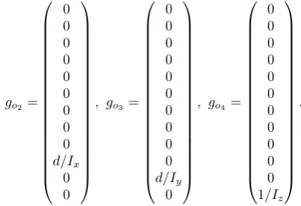
go2 =                     0 0 0 0 0 0 0 0 0 d/Ix 0 0                    

, go3 =                     0 0 0 0 0 0 0 0 0 0 d/Iy 0                    

, go4 =                     0 0 0 0 0 0 0 0 0 0 0 1/Iz

                    .

x0, y0 and z0 are the three coordinates of the absolute

[image:4.595.60.274.52.198.2]

ĨƌŽŶƚƌŽƚŽƌ ďĂĐŬƌŽƚŽƌ ůĞĨƚƌŽƚŽƌ ƌŝŐŚƚƌŽƚŽƌ ǇĂǁ͗ ƌŽůů͗ ƉŝƚĐŚ͗ x y z

Fig. 3. Dynamic model of quadrotor

position of the quadrotor helicopter. ψ, θ and φ are the three Euler’s angles of the attitude. These angles are yaw angle (−π < ψ < π), pitch angle (−π/2 < θ < π/2) and roll angle (−π/2 < φ < π/2) respectively. v1, v2 and v3

are the absolute velocities of the quadrotor helicopter with respect to an earth fixed inertial reference frame.p,qandr

are the angular velocities expressed with respect to a body reference frame. (Ax, Ay, Az) and (Ap, Aq, Ar) are the

resulting aerodynamics forces and moments acting on the quadrotor helicopter.Ix,IyandIzare the moment of inertia

with respect to the axes. m is the mass, g is the gravity constant and d is the distance from the center of mass to the rotors.u1 is the resulting thrust of the four rotors.u2 is

the difference of thrust between the left rotor and the right rotor. u3 is the difference of thrust between the front rotor

and the back rotor.u4is the difference of torque between the

two clockwise turning rotors and the two counter-clockwise turning rotors.

We design a static state feedback controller [16] of the quadrotor helicopter model.

uo=αo(x) +βo(x)vo (13)

whereα(x) =−A−o1(x)Bo(x),β(x) =A−o1(x),

Ao(x) =



  

G1 0 0 0

G2 0 0 0

G3 0 0 0

0 0 d(sinφsecθ)/Iy cosφsecθ/Iz



   ,

Bo(x) = L2foho1(x), L

2

foho2(x), L

2

foho3(x), L

2

foho4(x) T

,

vo is a controller of the linearized system with respect to

(12). The linearized system of (12) for all xis clearly not controllable sinceAo(x)is singular. To proceed, we need to

add some integrators of the inputuo1.

Using dynamic compensators with respect tou1 as

ζ=uo1, ξ= ˙ζ, µe1 = ˙ξ,

the quadrotor helicopter model (12) can be dynamic feedback linearizable. The other control inputs are also represented as

µe2 =uo2, µe3 =uo3, µe4 =uo4.

Then the extended model is obtained as

     ˙

x=fe(x) +

4

X

i=1 geiµei,

y=ho(x),

(14)

wherex= x0, y0, z0, ψ, θ, φ, v1, v2, v3, p, q, r, ζ, ξ

T

,

fe(x) =

                         v1 v2 v3

qsinφsecθ+rcosφsecθ qcosφ−rsinφ p+qsinθtanθ+rcosφtanθ

Ax/m+G1ζ Ay/m+G2ζ Az/m+g+G3ζ

Iy−Iz

Ix qr+Ap/Ix

Iz−Ix

Iy rp+Aq/Iy

Ix−Iy

Iz pq+Ar/Iz

ξ 0                          ,

ge1 = 0, 0, 0, 0, 0, 0, 0, 0, 0, 0, 0, 0, 0, 1 T

,

ge2 = 0, 0, 0, 0, 0, 0, 0, 0, 0, d/Ix, 0, 0, 0, 0 T

,

ge3 = 0, 0, 0, 0, 0, 0, 0, 0, 0, 0, d/Iy, 0, 0, 0 T

,

ge4 = 0, 0, 0, 0, 0, 0, 0, 0, 0, 0, 0, 1/Iz, 0, 0 T

.

We apply the I/O feedback linearization to the extended system (14). Then the controller is obtained as

µe=αe(x) +βe(x)ve

whereαe(x) =−A−e1(x)Be(x),βe(x) =A−e1(x),

Ae(x) =



  

a11 a12 a13 0 a21 a22 a23 0 a31 a32 a33 0 0 0 a43 a44



  

, Be(x) =



  

L4

feho1(x)

L4

feho2(x)

L4_f

eho3(x)

L2_f_eho4(x) 

   ,

aij =Lg_ojL3fehoi(x), i= 1,2,3, j= 1,2,3,

a4k =Lg_okLfeho4(x), k= 3,4.

The coordinate is obtained as

ze= ze1, ze2, ze3, ze4 T

,

IAENG International Journal of Applied Mathematics, 47:3, IJAM_47_3_16

(5)

where

ze1 = ho1, Lfeho1(x), L

2

feho1(x), L

3

feho1(x) T

,

2

feho2(x), L

3

feho2(x) T

,

2

feho3(x), L

3

feho3(x) T

,

ze4 = ho4, Lfeho4(x) T

.

The I/O linearized system is formulated as

˙

ze=Aze+Bve (15)

where A=    

A1 0 0 0

0 A1 0 0

0 0 A1 0

0 0 0 A2



  

, B =



  

B1 0 0 0

0 B1 0 0

0 0 B1 0

0 0 0 B2

    , C=    

C1 0 0 0

0 C1 0 0

0 0 C1 0

0 0 0 C2



  

, A1=



  

0 1 0 0

0 0 1 0

0 0 0 1

0 0 0 0



   ,

A2=

0 1 0 0

, B1= 0 0 0 1

T

, B2= 0 1

T ,

C1= 1 0 0 0, C2= 1 0.

Stabilization linear controller ve =−F ze of the linearized

system (15) is designed so that transfer function C(sI− A)−1B is Hurwitz.

IV. PML MODEL ANDTRAJECTORYTRACKING

CONTROLLERDESIGN OF THETRICYCLEROBOTMODEL

A. PML Model of the Tricycle Robot Model

We construct PML model [27] of the tricycle robot system (9). The state spaces of θ and w in the tri-cycle robot model (9) are divided by the 13 ver-tices x3 ∈ {−π,−5π/6, . . . , π} and the 13 vertices x4 ∈ {−3.0,−2.5, . . . ,3.0}. The state variable is x = (x1, x2, x3, x4, x5, x6)T = (x, y, θ, w, u1, v1)T.

˙ x=                

σ3+1 X

i3=σ3

wi3

3 (x3)f1(d3(i3))x5

σ3+1 X

i3=σ3

wi3

3 (x3)f2(d3(i3))x5

σ4+1 X

i4=σ4

wi4

4 (x4)f3(d4(i4))x5

0 x6 0                 +       0 0 0 0 0 1      

µ1+       0 0 0 1 0 0      

µ2.

(16)

We can construct PML models with respect tof1(x),f2(x)

and f3(x). The PML model structures are independent of

the vertex positionsx5andx6sincex5andx6are the linear

terms. This paper constructs the PML models with respect to the nonlinear terms ofx3 andx4.

Note that trigonometric functions of the tricycle robot (9) are smooth functions and are of classC∞. The PML models are not of classC∞. In the tricycle robot control, we have to calculate the third derivatives of the output y. Therefore the derivative PML models lose some dynamics. In this paper we propose the derivative PML models of the trigonometric functions.

B. Stabilizing Control Using Dynamic Feedback Lineariza-tion Based on PML Model

We define the output asη= (x1, x2)T in the same manner

as the previous section, the time derivative ofηis calculated as

˙ η =

Lfph1

Lfph2 = ˙ x1 ˙ x2 =

σ3+1 X

i3=σ3

wi3

3(x3)

f1(d3(i3))x5 f2(d3(i3))x5

where the vertices are f1(d3(i3)) = cosd3(i3) and

f2(d3(i3)) = sind3(i3). The time derivative of η doesn’t contain the control inputs (µ1, µ2). We calculate the time

derivative ofη˙. We get

¨

η1=L2fph1=

σ3+1 X

i3=σ3

wi3

3(x3)f1(d3(i3))x6

+

σ3+1 X

i3=σ3

wi3

3(x3)f 0

1(d3(i3))

σ4+1 X

i4=σ4

wi4

4 (x4)f3(d4(i4))x 2 5,

¨

η2=L2fph2=

σ3+1 X

i3=σ3

wi3

3(x3)f2(d3(i3))x6

+

σ3+1 X

i3=σ3

wi3

3(x3)f20(d3(i3))

σ4+1 X

i4=σ4

wi4

4 (x4)f3(d4(i4))x25,

wheref3(d4(i4)) = tan(Mtanhd4(i4))/L. We continue to calculate the time derivative ofη¨. We get

η₁(3)=L3fph1+Lg1L

2

fph1µ1+Lg2L

2

fph1µ2

=x3₅

σ3+1 X

i3=σ3

wi3

3 (x3)f 00

1(d3(i3))

σ4+1 X

i4=σ4

wi4

4(x4)f3(d4(i4))

!2

+3x5x6

σ3+1 X

i3=σ3

wi3

3(x3)f 0

1(d3(i3))

σ4+1 X

i4=σ4

wi4

4(x4)f3(d4(i4))

+

σ3+1 X

i3=σ3

wi3

3(x3)f1(d3(i3))µ1

+x2₅

σ3+1 X

i3=σ3

wi3

3 (x3)f10(d3(i3))

σ4+1 X

i4=σ4

wi4

4(x4)f30(d4(i4))µ2,

η₂(3)=L3_f

ph2+Lg1L

2

fph2µ1+Lg2L

2

fph2µ2

=x3₅

σ3+1 X

i3=σ3

wi3

3 (x3)f 00

2(d3(i3))

σ4+1 X

i4=σ4

wi4

4(x4)f3(d4(i4))

!2

+3x5x6

σ3+1 X

i3=σ3

wi3

3(x3)f 0

2(d3(i3))

σ4+1 X

i4=σ4

wi4

4(x4)f3(d4(i4))

+

σ3+1 X

i3=σ3

wi3

3(x3)f2(d3(i3))µ1

+x2₅

σ3+1 X

i3=σ3

wi3

3 (x3)f20(d3(i3))

σ4+1 X

i4=σ4

wi4

4(x4)f30(d4(i4))µ2.

IAENG International Journal of Applied Mathematics, 47:3, IJAM_47_3_16

(6)

The vertices f₁00(d3(i3)), f 00

2(d3(i3)) and The controller of

(16) is designed as

(µ1, µ2)T =−(LgL2fph)

−1_L3

fph+ (LgL

2

fph)

−1_v

=− _L

g1L

2

fph1 Lg2L

2

fph1

Lg1L

2

fph2 Lg2L

2

fph2

−1_L3

fph1

L3_f

ph2

+

_L

g1L

2

fph1 Lg2L

2

fph1

Lg1L

2

fph2 Lg2L

2

fph2 −1

v

wherev is the linear controller of the linear system (17).

(

˙

z=Az+Bu,

y=Cz, (17)

wherez= (h1, Lfph1, L

2

fph1, h2, Lfph2, L

2

fph2)

T _{∈ <}6_,

A=



      

0 1 0 0 0 0

0 0 1 0 0 0

0 0 0 0 0 0

0 0 0 0 1 0

0 0 0 0 0 1

0 0 0 0 0 0



      

, B=



      

0 0 0 0 1 0 0 0 0 0 0 1



      

, C=



      

1 0 0 0 0 0 0 1 0 0 0 0



      

T

.

Ifx56= 0, there exists a controller(µ1, µ2)T of the tricycle

robot model (16) since det(LgL2fph)6= 0.

In this case, the state space of the tricycle robot model is divided into13×13vertices. Therefore the system has12×12

local PML models. Note that all the linearized systems of these PML models are the same as the linear system (17).

In the same manner of (11), the dynamic feedback lin-earizing controller of the PML system is designed as

    

   

¨ u1=µ1,

u2=Msech2x4µ2,

µ1 µ2

=L3_f

ph+LgL

2

fhv.

(18)

The stabilizing linear controller v=−F z of the linearized system (17) is designed so that the transfer functionC(sI− A)−1_B _{is Hurwitz.}

Note that the dynamic controller (18) based on PML model is simpler than the conventional one (11). Since the nonlinear terms of controller (18) contain not the original nonlinear terms (e.g., sinx3, cosx3, tan(Mtanhx4)) but

the piecewise approximation models.

C. Trajectory Tracking Controller Based on PML System

We propose a tracking control [28] to the tricycle robot model (7). Consider the following reference signal model

(

˙ xr=fr,

ηr=hr.

The controller is designed to make the error signal e = (e1, e2)T = η−ηr → 0 as t → ∞. The time derivative

of eis obtained as

˙

e= ˙η−η˙r=

Lfphp1 Lfphp2

−

Lfrhr1

Lfrhr2

.

Furthermore the time derivative of e˙ is calculated as

¨

e=¨η−η¨r=

_L2

fphp1

L2

fphp2

−

L2_f_rhr1 L2

frhr2

Since the controllerµ doesn’t appear in the equation ¨e, we calculate the time derivative of¨e.

e(3)=η(3)−η(3)_r

=

_L3

fphp1

L3_f

php2

+LgL2fph

µ1 µ2

−

_L3

frhr1

L3_f

rhr2

The tracking controller is designed as

    

   

¨ u1=µ1,

u2=Msech2x4µ2,

µ1 µ2

=L3_f_ph−L3_f_rhr+LgL2fphv.

(19)

The linearized system (17) and controller v = −F z

are obtained in the same manners as the previous sub-section. The coordinate transformation vector is z = (e1, e˙1, ¨e1, e2, e˙2, e¨2)T.

Note that the dynamic controller (19) based on PML model is simpler than the conventional one on the same reason of the previous subsection.

V. PML MODEL ANDTRAJECTORYTRACKING

CONTROLLERDESIGN OF THEQUADROTORHELICOPTER

A. PML Model of the Quadrotor Helicopter

We construct PML model [29] of the quadrotor helicopter system (14). The state spaces ofψ,θandφin the quadrotor helicopter model (14) are divided by the following vertices.

x4=ψ∈ {−π,−5π/6,−2π/3, . . . , π},

x5=θ∈ {−5π/12,−δ1,−δ1/2,0, δ1/2, δ1,5π/12}, x6=φ∈ {−5π/12,−δ2,−δ2/2,0, δ2/2, δ2,5π/12}.

whereδ1 =δ2 =π/200. We construct the following PML

model of the quadrotor helicopter model (14).

  

 

˙

x=f(x) + 4

X

i=1 giµi,

y=h(x)

(20)

where

f(x) = x7, x8, x9, f4, f5, f6, f7, f8, f9, f10, f11, f12, x14,0

T ,

g1= 0, 0, 0, 0, 0, 0, 0, 0, 0, 0, 0, 0, 0, 1

T ,

g2= 0, 0, 0, 0, 0, 0, 0, 0, 0, Idx, 0, 0, 0, 0 T

,

g3=

0, 0, 0, 0, 0, 0, 0, 0, 0, 0, _Id

y, 0, 0, 0

T ,

g4= 0, 0, 0, 0, 0, 0, 0, 0, 0, 0, 0, _I1_z 0, 0

T

,

IAENG International Journal of Applied Mathematics, 47:3, IJAM_47_3_16

(7)

h(x) = h1, h2, h3, h4

T

= x1, x2, x3, x4

T

,

f4=x11

σ5+1 X

i5=σ5 σ6+1

X

i6=σ6

ωi5

5(x5)ω6i6(x6)f41(i5, i6)

+x12

σ5+1 X

i5=σ5 σ6+1

X

i6=σ6

ωi5

5 (x5)ωi66(x6)f42(i5, i6),

f5=x11

σ6+1 X

i6=σ6

ωi6

6 (x6)f51(i6)−x12

σ6+1 X

i6=σ6

ωi6

6(x6)f52(i6),

f6=x10+x11

σ5+1 X

i5=σ5 σ6+1

X

i6=σ6

ωi5

5 (x5)ω

i6

6(x6)f61(i5, i6)

+x12

σ5+1 X

i5=σ5 σ6+1

X

i6=σ6

ωi5

5 (x5)ω

i6

6(x6)f62(i5, i6),

f7=Ax/m+x13

σ4+1 X

i4=σ4 σ5+1

X

i5=σ5 σ6+1

X

i6=σ6

ωi4

4(x4)ω

i5

5 (x5)

×ωi6

6(x6)f7(i4, i5, i6),

f8=Ay/m+x13

σ4+1 X

i4=σ4 σ5+1

X

i5=σ5 σ6+1

X

i6=σ6

ωi4

4(x4)ω

i5

5(x5)

×ωi6

6(x6)f8(i4, i5, i6),

f9=Az/m+x13

σ5+1 X

i5=σ5 σ6+1

X

i6=σ6

ωi5

5(x5)ω6i6(x6)f9(i5, i6),

f10= Iy−Iz

Ix

x11x12+ Ap

Ix

, f11=

Iz−Ix

Iy

x12x10+ Aq

Iy

,

f12= Ix−Iy

Iz

x10x11+ Ar

Iz

.

In this paper, we construct the PML models with respect to trigonometric functions. Hence the state spaces of x4, x5 andx6 are divided into some vertices. For example, the

vertices f41(i5, i6) andf42(i5, i6) are given by substituting

the verticesx5andx6for the nonlinear termssinx6secx5(= sinφsecθ) andcosx6secx5(= cosφsecθ). Table I shows

the vertices of PML modelf41(i5, i6). In contrast, nonlinear

terms off10,f11 andf12 are not transformed into the PML

models. Since the nonlinear terms of f10, f11 and f12 are

multi-linear functions.

B. Stabilizing Control Using Dynamic Feedback Lineariza-tion Based on PML Model

The stabilizing conditions of PML system are represented by BMIs [23], therefore, it takes long computing time to obtain a stabilizing controller. In this paper, feedback lin-earization method is used for the controller design. Using the feedback linearization method as the controller designs, it is easy to design the continuous piecewise nonlinear controller for PML control system and the controller designs drastically reduce the time that it takes to find an optimal solution of the stabilizing condition by computer simulation. Therefore PML modeling and feedback linearizations could be a powerful combination for the analysis and synthesis of nonlinear control systems.

We define the output as η = (η1, η2, η3, η4)T =

(x1, x2, x3, x4)T, the time derivative ofη is calculated as

˙ η=



  

Lfh1 Lfh2 Lfh3 Lfh4



  

=



  

˙ x1

˙ x2

˙ x3

˙ x4



  

=



  

x7 x8 x9 f4



   .

The time derivative ofη doesn’t contain the control inputs

(u1, u2, u3, u4). We calculate the time derivative of η˙. We

get

¨

η1=L2fh1=f7, η¨2=L2fh2=f8, η¨3=L2fh3=f9,

¨

η4=L2fh4= ∂f4 ∂x5

f5+ ∂f4 ∂x6

f6+ ∂f4 ∂x11

f11+ ∂f4 ∂x12

f12

+ ∂f4 ∂x11

d/Iyµ3+ ∂f4 ∂x12

1/Izµ4,

where

∂f4 ∂x5

=x11

σ6 X

i6=σ6

ωi6

6(x6) (f41(σ5+ 1, i6)−f41(σ5, i6))/∆5

+x12

σ6 X

i6=σ6

ωi6

6(x6) (f42(σ5+ 1, i6)−f42(σ5, i6))/∆5,

∂f4 ∂x6

=x11

σ5 X

i5=σ5

ωi5

5(x5) (f41(i5, σ6+ 1)−f41(i5, σ6))/∆6

+x12

σ5 X

i5=σ5

ωi5

5(x5) (f42(i5, σ6+ 1)−f42(i5, σ6))/∆6,

∂f4 ∂x11

=

σ6+1 X

i6=σ6

ωi5

5 (x5)ω

i6

6(x6)f41(i5, i6),

∂f4 ∂x12

=

σ6+1 X

i6=σ6

ωi5

5 (x5)ω

i6

6(x6)f42(i5, i6),

∆5=d5(σ5+ 1)−d5(σ5), ∆6=d6(σ6+ 1)−d6(σ6).

We continue to calculate the time derivatives ofη¨1,η¨2 and ¨

η3. We get

η(3)₁ =L3_fh1= ∂f7 ∂x4

f4+ ∂f7 ∂x5

f5+ ∂f7 ∂x6

f6+ ∂f7 ∂x13

f13,

η(3)₂ =L3fh2= ∂f8 ∂x4

f4+ ∂f8 ∂x5

f5+ ∂f8 ∂x6

f6+ ∂f8 ∂x13

f13,

η(3)₃ =L3_fh3= ∂f9 ∂x5

f5+ ∂f9 ∂x6

f6+ ∂f9 ∂x13

f13,

where

∂fj

∂x4 =x13

σ5+1 X

i5=σ5 σ6+1

X

i6=σ6

ωi5

5 (x5)ω

i6

6(x6)

×(fj(σ4+ 1, i5, i6)−fj(σ4, i5, i6))/∆4,

∂fj

∂x5 =x13

σ4+1 X

i4=σ4 σ6+1

X

i6=σ6

ωi4

4 (x4)ωi66(x6)

×(fj(i4, σ5+ 1, i6)−fj(i4, σ5, i6))/∆5,

IAENG International Journal of Applied Mathematics, 47:3, IJAM_47_3_16

(8)

TABLE I

VERTICES OFPMLMODELf41(i5, i6)

f41 x6=−5π/12 x6=−δ2 x6=−δ2/2 x6= 0 x6=δ2/2 x6=δ2 x6= 5π/12

x5=−5π/12 −3.7321 −0.0607 −0.0303 0 0.0303 0.0607 3.7321

x5=−δ1 −0.9660 −0.0157 −0.0079 0 0.0079 0.0157 0.9660

x5=−δ1/2 −0.9660 −0.0157 −0.0079 0 0.0079 0.0157 0.9660

x5= 0 −0.9659 −0.0157 −0.0079 0 0.0079 0.0157 0.9659

x5=δ1/2 −0.9660 −0.0157 −0.0079 0 0.0079 0.0157 0.9660

x5=δ1 −0.9660 −0.0157 −0.0079 0 0.0079 0.0157 0.9660

x5= 5π/12 −3.7321 −0.0607 −0.0303 0 0.0303 0.0607 3.7321

∂fj

∂x6 =x13

σ4+1 X

i4=σ4 σ5+1

X

i5=σ5

ωi4

4(x4)ω5i5(x5)

×(fj(i4, i5, σ6)−fj(i4, i5, σ6+ 1))/∆6,

∂fj

∂x13 =

σ4+1 X

i4=σ4 σ5+1

X

i5=σ5 σ6+1

X

i6=σ6 ×ωi4

4 (x4)ωi55(x5)ω6i6(x6)fj(i4, i5, i6), ∂f9

∂x5 =x13

σ6+1 X

i6=σ6

ωi6

6 (x6) (f9(σ5+ 1, i6)−f9(σ5, i6))/∆5,

∂f9 ∂x6

=x13

σ5+1 X

i5=σ5

ωi5

5 (x5) (f9(i5, σ6)−f9(i5, σ6+ 1))/∆6,

∂f9 ∂x13

=

σ5+1 X

i5=σ5 σ6+1

X

i6=σ6

ωi5

5(x5)ω

i6

6(x6)f9(i5, i6),

j = 7,8. Since L3

fh1, L3fh2 and L3fh3 are independent of

the controlleru, we continue to calculate the time derivatives of η₁(3),η₂(3) andη₃(3).

η₁(4)=L4_fh1+Lg1L

3

fh1µ1+Lg2L

3

fh1µ2+Lg3L

3

fh1µ3,

η₂(4)=L4fh2+Lg1L

3

fh2µ1+Lg2L

3

fh2µ2+Lg3L

3

fh2µ3,

η₃(4)=L4_fh3+Lg1L

3

fh3µ1+Lg2L

3

fh3µ2+Lg3L

3

fh3µ3.

The details of the Lie derivatives are omitted due to lack of space. The controller of (20) is designed as

µ=α(x) +β(x)v

whereα(x) =−A−_qr1(x)Bqr(x),β(x) =A−qr1(x),

Aqr(x) =



  

Lg1L

3

fh1 Lg2L

3

fh1 Lg3L

3

fh1 0

Lg1L

3

fh2 Lg2L

3

fh2 Lg3L

3

fh2 0

Lg1L

3

fh3 Lg2L

3

fh3 Lg3L

3

fh3 0

0 0 Lg3Lfh4 Lg4Lfh4 

   ,

Bqr(x) = L4fh1, Lf4h2, L4fh3, L2fh4

T ,

v=−F zis the linear controller of the linear system (21).

(

˙

z=Az+Bu,

y=Cz, (21)

where

z= z1, z2, z3, z4

T ∈ <14_,

z1= h1, Lfh1, L2fh1, L3fh1

T

,

z2= h2, Lfh2, L2fh2, L3fh2,

T

,

z3= h3, Lfh3, L2fh3, L3fh3

T

,

z4= h4, Lfh4

T

,

A=blockdiag(A1, A2, A3, A4),

B= BT

1 B2T B3T B4T

T ,

C=blockdiag(C1, C2, C3, C4),

A1=



  

0 1 0 0

0 0 1 0

0 0 0 1

0 0 0 0



  

, A1=A2=A3, A4=

0 1 0 0

,

B1=



  

0 0 0 0

1 0 0 0



  

, B2=



  

0 0 0 0

0 1 0 0



   ,

B3=



  

0 0 0 0

0 0 1 0



  

, B4=

0 0 0 0

0 0 0 1

,

C1= 1 0 0 0, C1=C2=C3, C4= 1 0.

In this case, the state space of the quadrotor helicopter robot model is divided into13×7×7vertices. Therefore the system has12×6×6local PML models. Note that all the linearized systems of these PML models are the same as the linear system (21).

The dynamic feedback linearizing controller of the PML system (20) is designed as

(

¨ u1=µ1,

ui=µi, i= 2,3,4

(22)

The stabilizing linear controllerv =−F z of the linearized system (21) is designed so that the transfer functionC(sI− A)−1_B _{is Hurwitz.}

Note that the dynamic controller (22) based on PML model is simpler than the conventional one. Since the nonlinear terms of controller (22) contain not the original nonlinear terms (e.g.,sinφ,cosφ,secθ) but the piecewise approxima-tion models.

C. Trajectory Tracking Controller Based on PML System

We propose a trajectory tracking control to the quadrotor helicopter robot model (12). Consider the following reference

IAENG International Journal of Applied Mathematics, 47:3, IJAM_47_3_16

(9)

signal model

(

˙ xr=fr,

ηr=hr.

The controller is designed to make the error signal e = (e1, e2, e3, e4)T =η−ηr→0ast→ ∞. The time derivative

of eis obtained as

˙

e= ˙η−η˙r=



  

Lfh1 Lfh2 Lfh3 Lfh4



  

− 

  

Lfrhr1

Lfrhr2

Lfrhr1

Lfrhr2 

   .

Furthermore the time derivative of e˙ is calculated as

¨ e=



  

L2

fh1 L2

fh2 L2_fh3 L2

fh4+Lg3Lfh4u3+Lg4Lfh4u4 

  

− 

  

L2

frhr1

L2

frhr2

L2_f

rhr3

L2

frhr4 

   .

Since the controllerudoesn’t appear in the equationse¨1,e¨2

ande¨3 we calculate the time derivative of ¨ei (i= 1,2,3).



 

e(3)₁ e(3)₂ e(3)₃





=



 L3

fh1 L3

fh2 L3_fh3



−



 L3

frhr1

L3

frhr2

L3_f

rhr3





We continue to calculate the time derivatives of e(3)_i (i = 1,2,3).



 

e(4)₁ e(4)₂ e(4)₃





=



 L4

fh1 L4

fh2 L4_fh3



−



 L4

frhr1

L4

frhr2

L4_f

rhr3





+



 Lg1L

3

fh1µ1+Lg2L

3

fh1µ2+Lg1L

3

fh1µ3 Lg1L

3

fh2µ1+Lg2L

3

fh2µ2+Lg1L

3

fh2µ3 Lg1L

3

fh3µ1+Lg2L

3

fh3µ2+Lg1L

3

fh3µ3





The tracking controller is designed as

(

¨ u1=µ1,

ui=µi, i= 2,3,4.

(23)

The linearized system (21) and controller v = −F z

are obtained in the same manners as the previous sub-section. The coordinate transformation vector is z = (e1,e˙1,¨e1, e

(3)

1 , e2,e˙2,e¨2, e (3)

2 , e3,e˙3,¨e3, e (3)

3 , e4,e˙4)T.

Note that the dynamic controller (23) based on PML model is simpler than the conventional one on the same reason of the previous subsection.

VI. SIMULATION RESULTS

We apply the trajectory tracking control to the tricycle robot model (7) and the quadrotor helicopter model (12). Although the controller is simpler than the conventional I/O feedback linearization controller, the tracking performance based on PML model is the same as the conventional one. In addition, the controller is capable to use a nonlinear system with chaotic behavior as the reference model.

A. Tricycle Model

In the following simulations, the tricycle length L is 1.0 [m] and the angle constrainM isπ/3 [rad.].

1) Ellipse-shaped Reference Signal: Consider an ellipse model as the reference trajectory.

xr1

xr2

=

R1cosθ+xr1(0)

R2sinθ+xr2(0)

,

where R1 and R2 are the semiminor axes and (xr1(0), xr2(0)) is the center of the ellipse. Fig. 4

shows the simulation result. The dotted line is the reference signal and the solid line is the tricycle tracking trajectory. The semiminor parameters R1 and R2 are 10 and 25.

The initial positions are set at (x(0), y(0)) = (5,0) and

(xr(0), yr(0)) = (10,0). Fig. 5 shows the control inputsu1

andν1 of the tricycle. Fig. 6 shows the error signals of the

tricycle position(x, y).

2) Trajectory Tracking Control Using Some Ellipse-shaped Reference Signals: Arbitrary tracking trajectory con-trol can be realized using the ellipse-shaped tracking trajec-tory method. The controller design procedure is as follows:

1) Assign passing points(px(i), py(i)),i= 1, . . . , n.

We consider the passing points: (0,0), (10,20),

(26,30),(18,50)and(2,70)

2) Construct some ellipses trajectories to connect the passing points smoothly.

From (0,0)to(10,20), the trajectory 1:

xr1

xr2

=

10 cosθr+ 10

20 sinθr

, (24)

whereπ/2≤θr≤π.

xr1

xr2

=

16 cosθr+ 10

10 sinθr+ 30

, (25)

where−π/2≤θr≤0.

xr1

xr2

=

8 cosθr+ 18

20 sinθr+ 30

, (26)

where0≤θr≤π/2.

xr1

xr2

=

16 cosθr+ 18

10 sinθr+ 60

, (27)

where−π/2≤θr≤ −π/2.

3) Design the controllers (19) for the ellipse tracking trajectories (24)-(27).

We show a tracking trajectory control example for the tricycle robot system. Fig. 7 shows the reference signals (24)-(27) and the tricycle tracking trajectory. The dotted line is the reference signal and the solid line is the tricycle tracking trajectory. Fig. 8 shows the control inputs u1 and ν1 of the

tricycle. Fig. 9 shows the error signals with respect to the tricycle position(x, y).

B. Quadrotor Helicopter Model

1) Spiral descent reference trajectory: We consider two tracking trajectories as the reference signals. Although the controllers are simpler than the conventional I/O feedback linearization controllers, the tracking performance based on PML model is the same as the conventional one [16].

IAENG International Journal of Applied Mathematics, 47:3, IJAM_47_3_16

(10)

−30 −20 −10 0 10 20 30 −25

−20 −15 −10 −5 0 5 10 15 20 25

x [m]

[image:10.595.315.538.73.250.2]

y [m] (5,0) (10,0)

Fig. 4. Ellipse-shaped reference signal and the tricycle tracking trajectory

0 50 100 150 200

0.2 0.4 0.6 0.8 1

u 1

0 50 100 150 200

−0.04 −0.02 0 0.02 0.04

[image:10.595.56.282.74.254.2]

ν1

Fig. 5. Control inputsu1 andν1 of the tricycle

0 50 100 150 200

−5 0 5

error of x

0 50 100 150 200

−5 0 5

error of y

t

Fig. 6. Error signals of the tricycle position(x, y)

−30 −20 −10 0 10 20 30 40 50 60

0 10 20 30 40 50 60 70

x [m]

y [m]

Trajectory 1 Trajectory 2

(0,0)

(10,20)

[image:10.595.310.540.321.496.2]

(26,30) (18,50) (2,70)

Fig. 7. Reference signals (24)-(27) and the tricycle tracking trajectory

0 20 40 60 80 100 120 140 160 180 200

0.2 0.3 0.4 0.5 0.6 0.7

u1

[m]

0 20 40 60 80 100 120 140 160 180 200

−0.02 −0.01 0 0.01 0.02

ν1

[m]

x [m]

Fig. 8. Control inputsu1andν1of the tricycle

0 50 100 150 200

−5 0 5

error of x [m]

0 50 100 150 200

−5 0 5

error of y [m]

time

Fig. 9. Error signals of the tricycle position(x, y)

IAENG International Journal of Applied Mathematics, 47:3, IJAM_47_3_16

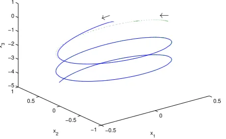
[image:10.595.50.287.326.499.2] [image:10.595.313.541.569.746.2] [image:10.595.61.287.573.745.2]

(11)

Consider a spiral-shaped reference trajectory [16] as the reference model.

  

 

xd1 =

1 2cos

t

2, xd2 =

1 2sin

t 2, xd3 =−1−

t

10, xd4 =

π 3.

(28)

The feedback gain is calculated as

F =



  

F1 0 0 0

0 F1 0 0

0 0 F1 0

0 0 0 F2



   ,

F1= 1.000,3.078,4.236,3.078

,

F2= 1.000,1.732

.

The helicopter is initially in hover flight and the ini-tial positions are set at (x1, x2, x3, x4) = (0,0,0,0) and (xr1, xr2, xr3, xr4) = (1/2,0,1, π/3). In this simulation, the

parameters are given by m= 0.7,Ix =Iy =Iz = 1.242,

d = 0.3 and g = 9.81. Fig. 10 shows the trajectory signals. The solid line is the state response (x1, x2, x3) of

the helicopter and the dotted line is the reference signal (28).

2) Spiral ascending reference trajectory: Consider a spiral-shaped reference trajectory [16] as the reference model.

  

 

xd1 =

1 2cos

t

2, xd2 =

1 2sin

t 2, xd3 =1 +

t

10, xd4=

π 3.

(29)

The feedback gain is the same as the previous example. The helicopter is initially in hover flight and the ini-tial positions are set at (x1, x2, x3, x4) = (0,0,0,0) and (xr1, xr2, xr3, xr4) = (1/2,0,1, π/3). In this simulation, the

parameters are given by m= 0.7,Ix =Iy =Iz = 1.242,

d = 0.3 and g = 9.81. Fig. 11 shows the trajectory signals. The solid line is the state response (x1, x2, x3) of

the helicopter and the dotted line is the reference signal (29). These results confirm the feasibility of the tracking con-trol performance. Although the PML model (20) and the controller (19) are simpler than the conventional dynamic feedback linearization controller and model [16], the control performance based on PML model is the same as the conventional one [16].

−0.5

0

0.5

−1 −0.5 0 0.5 1 −5 −4 −3 −2 −1 0 1

x 1 x

2 x3

←

[image:11.595.280.534.54.201.2]

←

Fig. 10. Decent reference trajectories

−1 −0.5

0 0.5

1

−0.5 0

0.5 0 1 2 3 4 5

x 1 x

2

x3

← ←

Fig. 11. Ascending reference trajectories

3) Trajectory Tracking Control Using Some Ellipse-shaped Reference Signals: Arbitrary tracking trajectory con-trol can be realized using the ellipse-shaped tracking trajec-tory method. The controller design procedure is as follows: 1) Assign passing points (px(i), py(i), pz(i)), i =

1, . . . , n. We consider the passing points: (0,0,0),

(5,0,2),(4,0,3) and(0,0,0).

2) Construct these trajectories to connect the passing points smoothly.

From (0,0,0)to(5,0,2), the trajectory 1 is



 xr1

xr2

xr3 

=





5 sinθrcosϕr

sinθrsinϕr

2 cosθr+ 2



, (30)

whereπ/2≤θr≤π andϕ= 0.



 xr1

xr2

xr3 

=





1 2cost+

9 2 1 2sint 2 + t

5π



. (31)



 xr1

xr2

xr3 

=





4 sinθrcosϕr+ 4

sinθrsinϕr

3 cosθr



, (32)

where−π/2≤θr≤0 andϕr= 0.

3) Design the controllers (23) for the ellipse tracking trajectories (30)-(32).

We show the simulation result for the quadrotor helicopter system. Fig. 12 shows the reference signals (30)-(32) and the quadrotor helicopter tracking trajectory. The dotted line is the reference signal and the solid line is the tricycle tracking trajectory.

VII. CONCLUSIONS

We have proposed the trajectory tracking controller de-signs of a tricycle robot and a quadrotor as non-holonomic systems based on PML models. The approximated model are fully parametric. I/O dynamic feedback linearization is applied to stabilize PML control system. PML modeling with feedback linearization is a very powerful tool for analyzing and synthesizing nonlinear control systems. We also have designed the tracking controllers to the tricycle robot and the quadrotor. Although the controllers are simpler than the conventional I/O feedback linearization controller, the

IAENG International Journal of Applied Mathematics, 47:3, IJAM_47_3_16

[image:11.595.48.279.610.752.2]

(12)

0 1

2 3

4

5 −1

0

1 0

0.5 1 1.5 2 2.5 3 3.5

Trajectory 1

(0,0,0)

(5,0,2) (4,0,3)

x1

x2

[image:12.595.54.289.85.239.2]

x3

Fig. 12. Reference signals (30)-(32) and the tracking trajectory of the quadrotor helicopter system

tracking performance based on PML model is the same as the conventional one. The examples have been shown to confirm the feasibility of our proposals by computer simulations.

REFERENCES

[1] R. W. Brockett,Asymptotic stability and feedback stabilization,

Dif-ferential Geometric Control Theory. Boston: Birkh¨auser, 1983, pp.

181–191.

[2] B. d’Andr´ea-Novel, G. Bastin, and G. Campion, “Modeling and control of non holonomic wheeled mobile robots,” inthe 1991 IEEE

International Conference on Robotics and Automation, 1991, pp.

1130–1135.

[3] K. Kimura, S. Nozawa, Y. Kakiuchi, K. Okada, and M. Inaba, “Tricycle manipulation strategy for humanoid robot based on active and passive manipulators control,” pp. 5797–5804.

[4] F. Kallasi, D. L. Rizzni, F. Oleari, M. Magnani, and S. Caselli, “A novel calibration method for industrial agvs,”Robotics and

Au-tonomouse Systems, vol. 94, pp. 75–88, 2017.

[5] R. Fierro and F. L. Lewis, “Control of a nonholonomic mobile robot: backstepping kinematics into dynamics,” inthe 34th Conference on

Decision and Control, 1995, pp. 3805–3810.

[6] T.-C. Lee, K.-T. Song, C.-H. Lee, and C.-C. Teng, “Tracking con-trol of unicycle-modeled mobile robots using a saturation feedback controller,”IEEE Transactions on Control Systems Technology, vol. 9, no. 2, pp. 305–318, 2001.

[7] J. Guldner and V. I. Utkin, “Stabilization of non-holonomic mobile robots using lyapunov functions for navigation and sliding mode control,” inthe 33rd Conference on Decision and Control, 1994, pp. 2967–2972.

[8] J. Yang and J. Kim, “Sliding mode control for trajectory tracking of nonholonomic wheeled mobile robots,”IEEE Transactions on Robotics

and Automation, pp. 578–587, 1999.

[9] B. d’Andr´ea-Novel, G. Bastin, and G. Campion, “Dynamic feedback linearization of nonholonomic wheeled mobile robot,” inthe 1992

IEEE International Conference on Robotics and Automation, 1992,

pp. 2527–2531.

[10] G. Oriolo, A. D. Luca, and M. Vendittelli, “WMR control via dynamic feedback linearization: Design, implementation, and experimental val-idation,”IEEE Transaction on Control System Technology, vol. 10, no. 6, pp. 835–852, 2002.

[11] E. Yang, D. Gu, T. Mita, and H. Hu, “Nonlinear tracking control of a car-like mobile robot via dynamic feedback linearization,” in

University of Bath, UK, no. ID-218, 2004.

[12] A. D. Luca, G. Oriolo, and M. Vendittelli, “Stabilization of the unicy-cle via dynamic feedback linearization,” inthe 6th IFAC Symposium

on Robot Control, 2000.

[13] R. Xu and U. ¨Ozg¨uner, “Sliding Mode Control of a Quadrotor Heilicopter,” inProceedings of the 45th IEEE Conference on Decision

& Control, 2006, pp. 4957–4962.

[14] A. Gessow and G. Myers, Aerodynamics of the helicopter, third edition ed. New York: Frederick Ungar Publishing Co., 1967.

[15] E. Altug, J. P. Ostrowski, and R. Mahony, “Control of a Quadrotor Helicopter Using Visual Feedback,” inProceedings of the 2002 IEEE

International Conference on Robotics & Automation, 2002, pp. 72–77.

[16] V. Mistler, A. Benallegue, and N. M’Sirdi, “Exact linearization and noninteracting control of a 4 rotors helicopter via dynamic feedback,”

in IEEE International Workshop on Robot and Human Interactive

Communication, 2001, pp. 586–593.

[17] M. Bouchoucha, S. Seghour, and M. Tadjine, “Classical and Second Order Sliding Mode Control Solution to an Attitude Stabilization of a Four Rotors Helicopter : from Theory to Experiment,” inProceedings

of the 2011 IEEE International Conference on Mechatronics, 2011,

pp. 162–169.

[18] A. Benallegue, A. Mokhtari, and L. Fridman, “Feedback Linearization and High Order Sliding Mode Observer For A Quadrotor UAV,” in Proceedings of the 2006 International Workshop on Variable Structure

Systems, 2006, pp. 365–372.

[19] L. Derafa, L. Fridman, A. Benallegue, and A. Ouldali, “Super Twisting Control Algorithm for the Four Rotors Helicopter Attitude Tracking Problem,” in11th International Workshop on Variable Structure Sys-tems, 2010, pp. 62–67.

[20] C. Zhang, X. Zhou, H. Zhao, A. Dai, and H. Zhou, “Three-dimensional fuzzy control of mini quadrotor uav trajectory tracking under impact of wind disturbance,” inProceedings of the 2016 International

Con-ference on Advanced Mechatronic Systems, 2016, pp. 372–377.

[21] J. Hwangbo, I. Sa, R. Siegwart, and M. Hutter, “Control of a quadrotor with reinforcement learning,”IEEE Robotics and Automation Letters, vol. 2, no. 4, pp. 2096–2103, 2017.

[22] M. Sugeno, “On stability of fuzzy systems expressed by fuzzy rules with singleton consequents,”IEEE Trans. Fuzzy Syst., vol. 7, no. 2, pp. 201–224, 1999.

[23] K.-C. Goh, M. G. Safonov, and G. P. Papavassilopoulos, “A global optimization approach for the BMI problem,” inProc. the 33rd IEEE CDC, 1994, pp. 2009–2014.

[24] T. Taniguchi and M. Sugeno, “Piecewise bilinear system control based on full-state feedback linearization,” inSCIS & ISIS 2010, 2010, pp. 1591–1596.

[25] ——, “Stabilization of nonlinear systems with piecewise bilinear models derived from fuzzy if-then rules with singletons,” in

FUZZ-IEEE 2010, 2010, pp. 2926–2931.

[26] ——, “Design of LUT-controllers for nonlinear systems with PB models based on I/O linearization,” inFUZZ-IEEE 2012, 2012, pp. 997–1022.

[27] ——, “Trajectory tracking controller design for a tricycle robot using piecewise multi-linear models,” inLecture Notes in Engineering and Computer Science: Proceedings of The International MultiConference of Engineers and Computer Scientists 2017,15-17 March, 2017, Hong Kong, 2017, pp. 188–193.

[28] T. Taniguchi, L. Eciolaza, and M. Sugeno, “Look-Up-Table controller design for nonlinear servo systems with piecewise bilinear models,”

inFUZZ-IEEE 2013, 2013.

[29] ——, “Quadrotor control using dynamic feedback linearization based on piecewise bilinear models,” in 2014 IEEE Symposium Series on

Computational Intelligence, 2014.

Tadanari Taniguchi receive the Doctor of Engineering degree from the

University of Electro-Communications, Tokyo, Japan, in 2001. He was born in Toyama, Japan, in 1971. He graduated from the University of Electro-Communications. His research interests include intelligent control and nonlinear control. From 2001 to 2005, he was a research scientist at Brain Science Institute, RIKEN, Japan. Then he has served Tokai University, Kanagawa, Japan since 2005. He was a Visiting Scientist with Universite de Valenciennes, France, in 2015. He is currently an Associate Professor of Tokai University. He received a Best Paper Award of The 2017 IAENG International Conference on Control and Automation.

IAENG International Journal of Applied Mathematics, 47:3, IJAM_47_3_16

(13)

Michio Sugenowas born in Yokohama, Japan, in 1940. He graduated from the Department of Physics, The University of Tokyo, Tokyo, Japan. He then worked with Mitsubishi Atomic Power Industry. Then, he served the Tokyo Institute of Technology as a Research Associate, an Associate Professor, and a Professor from 1965 to 2000. After retiring from the Tokyo Institute of Technology, he was a Laboratory Head at the Brain Science Institute, RIKEN, from 2000 to 2005, and then, as a Distinguished Visiting Professor with Doshisha University from 2005 to 2010. He is currently an Emeritus Professor with the Tokyo Institute of Technology, Tokyo. Dr. Sugeno was the President of the Japan Society for Fuzzy Theory and Systems from 1991 to 1993, and also the President of the International Fuzzy Systems Association from 1997 to 1999. He is the first recipient of the IEEE Pioneer Award in Fuzzy Systems with Zadeh in 2000. He also received the 2010 IEEE Frank Rosenblatt Award and Kampt de Ferit Award in 2012.