implications of

J. Range Manage.

56: 418-424 September 2003

Economic implications of off-stream water developments to improve riparian grazing

AMY M. STILLINGS, JOHN A. TANAKA, NEIL R. RIMBEY, TIMOTHY DELCURTO, PATRICK A. MOMONT, AND MARNI L. PORATH

Stillings was former Graduate Research Assistant, Department of Agricultural and Resource Economics, Oregon State University, Corvallis, Ore. 97331 and currently Policy Analyst, M.J. Bradley

Associates, Inc., Concord, Mass.; Tanaka is Associate Professor, Agricultural and Resource Economics, Oregon State University; Rimbey is Professor, Agricultural Economics and Rural Sociology, University of Idaho, Caldwell, Ida.; DelCurto ^is Associate Professor, Animal Sciences, Oregon State University; Momont is Associate Professor, Animal Science, University of Idaho; and Porath (nee Dickard) is former Graduate Research Assistant, Animal Science, University of Idaho and currently is an Extension Agent/Assistant Professor, Oregon State University, Lakeview, Ore.

Abstract

Livestock grazing in riparian areas is an important manage- ment issue on both private and public lands. A study was initiat- ed in northeastern Oregon to evaluate the economic and ecologi- cal impacts of different cattle management practices on riparian areas. The effect of off-stream water and salt on livestock distrib- ution and subsequent impact on riparian use, water quality, and livestock production was evaluated. ^A multi-period bioeconomic linear programming model is used to evaluate the long-term eco- nomic feasibility of this management practice with a riparian uti- lization restriction of 35% for a 300 cow-calf operation. The uti- lization restriction resulted in economically optimal herd sizes 10% smaller than the baseline herd size. With the management practice, cattle were distributed more evenly, consumed more upland forage before maximum riparian utilization was reached, and gained more weight. The economic impacts of these out- comes were increased with expected annual net returns to the ranch for the project ranging between $4,500 and $11,000 depending on cattle prices and precipitation levels.

Properly functioning riparian systems are vital to the health of watersheds and provide an important forage and habitat resource for livestock and wildlife. Recent concerns about water quality and wildlife and fisheries habitat have focused attention on live- stock management practices occurring within these areas. The impacts of livestock on riparian systems have been identified (Kauffman and Krueger 1984) and specialized management strategies such as rest rotation, late season grazing and riparian corridor fencing have been developed. However, economic assessments of these management alternatives are often lacking (Skovlin 1984, Armour et al. 1991). When economic analyses are undertaken, projects are often found to not be economically justi- fied (Nielsen 1984, Workman 1986). There is a critical need at this time for economically feasible riparian grazing management strategies that achieve environmental goals.

Bioeconomic models are one method that can be used for eval- uating management options. They can combine biological

Financial support was provided by the USDA Sustainable Agriculture Research and Extension (SARE) program and the Blue Mountains Natural Resources Institute, La Grande, Ore. Oregon State University Extension and Experiment Station Technical Paper Number 11958.

Manuscript accepted

Nov. 02.

Resumen

El apacentamiento de ganado en areas riberenas es un impor- tante problema de manejo en terrenos publicos y privados. Se inicio un estudio en el noreste de Oregon para evaluar ^los impactos economicos _y economcos de diferentes practicas de manejo de ganado en areas riberenas. Se evaluo el efecto de la disponibilidad de agua _y sal lejos de la corriente en la distribu- cion del ganado _{y los} impactos subsecuentes en ^el use del area riberena, la calidad del agua _y la produccion del ganado. ^Se use un modelo de programacion lineal de multiperiodos bioeconomi- cos para evaluar la factibilidad economica a largo plazo de esta practica de manejo con una restriccion de utilizacion del area riberena del 35 % para una operacion de 300 pares de vaca- becerro. La restriccion de utilizacion resulto en tamanos de hato economicamente optimos 10% menores que el tamano base del hato. Con la practica de manejo el ganado se distribuyo mas uni- formemente y consumio mas forraje de las areas tierras arriba antes de alcanzar la maxima utilizacion del area riberena _y gang mas peso. Los impactos economicos de estos resultados fueron incrementos del retorno neto anual esperado del rancho en un rango de $ 4,500 a $ 11,000 dolares dependiendo de los precios _y niveles de precipitation.

dynamics with economic behavior to help determine an optimal bioeconomic strategy. Standiford and Howitt (1992) developed such a model to evaluate ranch enterprises on California range- lands by incorporating tree canopy, forage and livestock dynam- ics. Dynamic models have also been developed by Pope and McB ryde (1984) and Torell et al. (1991) to determine the intertemporal influence of stocking rates on current and future forage and livestock production.

In this paper, a bioeconomic linear programming model is developed to determine the economic impacts of a grazing man- agement strategy on a 300-head cow-calf ranch. The strategy under evaluation is the placement of an alternative water source and trace mineralized salt in the upper portion of pastures which is designed to influence cattle distribution between riparian and upland areas. A field test of the dispersion project was conducted and the data were used in the development of the bioeconomic model. The purpose of the economic analysis is to compare the optimal (profit maximizing) net returns of a ranch operating with and without off-stream water and salt under varying crop year precipitation levels and market prices (states of nature).

418 JOURNAL OF RANGE MANAGEMENT 56(5) September 2003

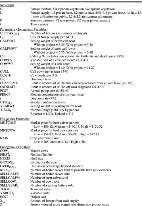
Table 1. Variable names, definitions, and values used in the ranch model.

Subscripts

G Forage location: G

riparian vegetation, G2 upland vegetation

L Forage supply: L1 private land, L2 public lease 35%, L3 private lease, L4 hay, L5 over utilization on public. L2 & L5 are summer allotments.

P Summer pastures: P1 non-project, P2 water project pasture

t Time (years)

Parameters

Exogenous Variables

HECTAREG,P Number of hectares in summer allotments CL Cost of forage supply per AUD CALFFWT Selling weight of heifer calf (cwt)

Without project = 5.25, With project = 5.38 CALFMWT Selling weight of steer calf (cwt)

Without project = 5.75, With project = 5.88

CLF Calving % (includes conception rate, birth rate and death loss) (88%) COWCST Variable cost of a cow per month ($14.41)

COWWT Selling weight of a cow (cwt)

Without project =11.0, With project =11.27 CULL Cull cow rate (at least 15%)

DEATH Cow death rate (1%)

DFL

Discount factor

LEASELMT Limit to amount of AUDs that can be purchased from private lease (10,350) OWNLMT Limit to amount of AUDs off own rangeland (31,470)

POST Annual pump cost ($438.40)

PRECP Median precipitation of crop year (mm)

r Discount rate (7%)

UTILG _P Standard utilization levels

YEARWT Selling weight of yearling heifer (cwt) YIELDS Normal forage yield (dry kg per ha)

Riparian =1,301, _{Upland =} 811 Exogenous Parameter

MKTCALF Market price for beef calves per cwt MKTCOW

RAIN

Low ₌ $86.12, Median ₌ $100.13, High ₌ $120.32 Market price for beef cows per cwt

Low ₌ $54.82, Median = $59.81, High = $72.13 Crop year rain in mm

Low ₌ 265, Median ₌ 320, High ₌ 380 Endogenous Variables

COWL FIRSTL HERDt INCOMEL OVERG,P2,t REPLL SELLCALFFL SELLCALFML SELLCOWL SELLYEARL TERM VARCSTL PCST

z

Mature cows First calf heifers Herd size Income for the year

Utilization percentage beyond standard

Number of heifer calves held as possible herd replacements Number of heifer calves sold

Number of steer calves sold Number of cows sold Number of yearling heifers sold Terminal value

Variable costs Project cost

Amount of forage from each supply

Present value of gross margin less dispersion project costs

Model Design

The off-stream water bioeconomic model consists of a set of relationships depicting the objective function, cattle herd equations of motion, and forage growth equations of motion. The model is solved over a 60-year planning horizon.

Objective Function

The objective function (equation ¹⁾ of the ranch is to maximize the discounted total gross margin and terminal value less dispersion project costs over a planning horizon of T years. A discount factor (DFt)

of 7% is used in present value calculations.

Table

gives the definitions for all van -

ables and subscripts used in the paper.

T

Max Z = ^{DFS *} (INCOMES

t=1

VARCSTS

PCST) + TERM (1) Livestock revenue (INCOMES), shown in equation 2, is a function of the number of cattle sold, weight of the cattle and the market price received. The market prices were 5 year average prices for Oregon cat- tle, weighted by class of cattle expected in the herd.

INCOMES = (SELLCOWT ^{* COWWT +}

SELLYEARS ^* YEARWT) (2)

* MKTCOW + (SELLCALFFS ^* CALFFWT + SELLCALFMS

* CALFMWT) ^* MKTCALF

The numbers of cattle sold in each age class (SELLCOWS, SELLYEARS, SELLCALFFS and SELLCALFMS) are choice variables within the model and optimal numbers of animals for sale are determined. The weights of cattle (COWWT, CALFFWT and CALFMWT) were defined to be different for the various management schemes stud- ied. Yearling replacement heifers were not considered as sale animals so their weight was not different between treatments. The selling prices (MKTCOW and MKTCALF) that ranchers receive for their product are a source of risk. To account for this risk, 3 parameter values are assigned from the his- torical price data set of the region to repre- sent low, median and high market prices.

The annual total variable costs

(VARCSTS) of the livestock enterprise, shown in equation ^3, include both variable costs (COWCST) and variable feed costs (CL).

VARCSTS =12 ^* (COWL + FIRSTS) ^* COWCST +

S

YXL,t * CL t=

(3)

Variable costs per cow are based on a 300 head cow-calf enterprise budget for the mountain region of northeast Oregon (Turner et al. 1998) where the dispersion project study was located. Total feed cost is dependent upon a number of factors. The annual off-stream water and salt project cost (PCST) is an exogenously given para- meter derived from the initial investment costs amortized over the life of the invest- ment plus the variable costs associated with the riparian improvement system.

Equation 4 denotes the terminal value. It is calculated as the present value of an infinite series of net revenue multiplied by the number of animals in the herd in the last year. The exogenous parameter value (NETREV) is calculated from the enter- prise budget using the low, median and high market prices depending upon the price condition considered. The parameter HERD is defined below as the number of mature cows, first-calf heifers, and replacement heifers. The purpose of the TERM variable is to force the model to consider future production. In many multi- period models, the tendency is to liquidate the herd near the end in order to maximize net income. Including the terminal value in the model assumes that the ranch will

JOURNAL OF RANGE MANAGEMENT 56(5) September 2003 419

continue into perpetuity at the final pro- duction level and represents the produc- tion value of the ranch beyond year T.

TERMT = ((HERDT -SELLCOWT -SELLYEART) *NETREV)

* (r * _{(1-1((1 +} r)^T))-1)-1 (4)

Cattle Equations of Motion

Cow/calf production is based on typical ratios between different animal classes as defined in Turner et al. (1998). There are 4 age classes on the ranch: calf, yearling replacement heifer, first calf heifer and mature cow. All replacement heifers are retained from the calf crop. The calf wean- ing success rate (CLF) is assumed to be 88%. This is based on a 95% conception rate for cows (all replacement heifers were pregnancy tested in the fall), a 2% death loss during calving and a 5% calf loss after birth (Turner et al. 1998). In November, heifer calves can be sold (SELLCALFFL) or kept as heifer replace- ments for the next year (REPLt+1) as rep- resented in equation 5. All steer calves are sold after weaning in the fall (equation 6).

SELLCALFFt ₌ (COWL + FIRST') ^*

CLF ^* 0.5 - REPLL+I (5)

SELLCALFMt = (COW' ⁺ FIRST)

* CLF ^* 0.5 (6)

For the year after their birth, retained heifer calves (REPLt) are considered part of the herd as yearlings. After being preg- nancy tested in the fall, these possible replacements are either sold as yearling heifers (SELLYEARt) or kept as part of the herd for the next year (FIRSTt+I) as shown in equation 7.

REPL' = FIRSTt+1 + SELLYEARt (7) Due to low conception rates and the desire to keep only the best replacements, it is assumed that at least 25% of the possible

heifer replacements are culled in November (equation 8).

SELLYEARt > 0.25 ^* REPLL (8) The size of the herd (equation 9) is a func- tion of the previous year's cow herd, num- ber of replacements kept as first calf

heifers from the last 2 years and the num- ber of cows lost due to mortality or culling.

HERDL = COWL + FIRSTt + REPLt (9) Equation 10 represents the equation of motion for cows.

COWL+I = (COWL + FIRST )*

(1-DEATH) - SELLCOWL (10) The death loss rate (DEATH) is assumed

to be

%. Equation 11 sets the culling rate of mature cows to be at least 15% that is the typical rate of the study region (Turner

et al. 1998).

SELLCOWL > COWL ^* 0.15 (11) Calf survival rates are a function of the mother cow's age. To maintain the calf crop success rate of 88%, the herd is restricted by equation 12 to limit first calf heifers to less than one third of the number

of cows.

FIRSTL < (COWL + FIRSTL) *0.33 (12) Other resource constraints, represented by equation (13), such as ranch facilities and equipment, limit the herd (cows, first calf heifers and yearling heifers) to a total

of 500 animals.

HERDL < 500 (13)

Forage Equations of Motion

The typical rancher in the northeast Oregon mountain region supplies a 345 animal unit herd (300 cows at

animal unit (AU) and 60 yearlings at 0.75 AU) with hay _(XL4) for the duration of winter (Table 1), privately owned spring range and stringer meadows _(XL1) for 3 months and Forest Service lands _(XL2 and _XLS) for 4 months. The model also includes the option of leasing private pasture _(XL3).

There are 2 factors that influence the amount of forage available. The first is the amount of precipitation that falls during the crop year (September through June).

One study found that 75 to 90% of forage yield fluctuations could be attributed to variations in the amount of precipitation received during the crop year. Sneva and Hyder (1962) found that the response of forage yield to changes in precipitation is

consistent on a percentage basis even though productivity among study sites var- ied. The forecasting model they developed for range herbage production in eastern Oregon is incorporated in the model to adjust forage yields given precipitation parameters.

The number of animal unit days (AUD) available from privately owned pastures (XL1) and privately leased pastures _(XL3) are fixed at their long-term averages regardless of precipitation conditions, shown with equations 14 and 15, since the focus of the economic analysis is on sum- mer grazing when the dispersion project can be implemented.

XLI,t < 31,567 (14)

XL3,t <10,523 (15)

For a minimum duration of ⁵ months

(winter, 152 days), represented in equation 16, the herd is fed a mixture of native and alfalfa hay. Hay may be fed longer than 5

months if summer forage production is low or is needed to maintain a larger herd size.

XL4 t > (COWt+1 + FIRSTt+1

+ 0.75 ^* REPLt)* 152 (16) The second factor that determines for- age supply is the management decision of the forage utilization levels achieved on private and public pasturelands. In light of research that may link forage utilization level to habitat quality for wildlife and fisheries, the Forest Service is beginning to regulate the maximum utilization level (UTILg,p) of vegetation from their allot- ments. This model assumes that the uti- lization standards are 35% of riparian veg- etation (subscript _g ¹⁾ and 50% of upland forage (subscript g2). Federal grazing per- mits purchased by the model ranch allow for 1,380 AVMs to be consumed. This amount of forage provides feed for 345 animal units for 4 months at regulated uti- lization conditions when crop year precipi- tation is at normal levels. Changes in pre- cipitation will cause the quantity of forage produced from the Forest Service lands to vary. In years of low precipitation, the ranch manager must decide to decrease herd size, remove cattle early, and exceed the utilization standard or any combination of the 3.

There are consequences if the manager allows the utilization standard in the ripar- ian zone to be exceeded. The penalty used in this model was based on practices observed in the region. While penalties vary among administrative units, this model assumes the agency will revoke twice the percentage exceeded (OVERg,p,t) from the total permitted amount from the next year's permit. For example, if the monitored riparian pasture is grazed at a 45% utilization level, 10% more than the agency's desired level, then the agency will lower the total permitted number of AUMs by 20% for the next year. Again, the ranch manager would face a decision to reduce herd size, remove cattle early, or exceed the utilization percentage. (Note that the model design does not account for a penalty that is cumulative. It is unlikely that the agency would permit the rancher to continue to exceed the standard without enacting harsher penalties. While the penalty is not an entirely accurate depic- tion of actual practices, limits of the GAMS software dictated this approach.)

Data collected for this study was for the period of mid July through August, which was only 1.5 months of grazing out of the

420 JOURNAL OF RANGE MANAGEMENT 56(5) September 2003

usual 4 months of public land grazing. For analysis of the dispersion project, the pub- lic lease pastures are divided into

ripari- an pasture where the dispersion project can be implemented for 1.5 months (sub- script p2) and ² upland, non-riparian pas- tures with no dispersion project imple- mented (subscript _{p1). The} non-project pastures are restricted to the regulated lev- els. Thus, the utilization standards only apply to the pasture grazed from mid July to the end of August when off-stream water and salt could be provided.

Forage supplied from public lands is divided into 2 categories. _XL2 is vegetation consumed at or below the regulated utiliza- tion levels while _XL5 represents consump- tion above the limits. Using Sneva and Hyder's (1962) forage production forecast- ing model, equation 17 predicts the amount of forage available for consumption at desired Forest Service levels.

22

XL2,t

((RAINt ^* 12.591) ^*

g=1 g=1

111-10.6) ^* 100

^* YIELDg ^* (17) (25 ^* HECTAREg,p ^* (UTILg,p

- 2*OVERg1,p2,t-1))-1

The exogenous number of hectares of riparian and upland area in the pastures is designated as HECTAREg,p. Sneva and Hyder's (1962) regression equation for the forage yield index is (RAIN/12.59) ^* 111 - 10.6) ^* 1001 where RAINt is an exoge- nous parameter that can be set at a low, median or high value, depending upon the crop year precipitation condition desired.

The calculated amount of forage produced during a median year of crop year precipi-

tation (YIELDg) is divided by 11.36 kg/AUD to convert the equation into terms of animal unit days.

Nonproject pasture utilization (UTIL,p1) is set at the agency's desired utilization level of 35% riparian usage and 50% utilization for the uplands. Utilization on the second public lease pasture

(UTILg,p2) depends upon whether off- stream water and salt is provided. It also is an endogenous figure within the model set for the P2 pasture. The percent of the riparian vegetation that is consumed beyond 35% the previous year in the treat- ment period pasture, P2 (equation 18), is OVERg1,p2,t_1. It also acts as the agency's penalty and used in the calculation of available forage in equation 17. Equation

18 allows for grazing above the restricted levels and represents the forage available for consumption as _XL5.

22

XL5,t < ((RAINt ^{* 12.59}

g=1 p=1

* 111-10.6) * 100-1 * YIELD (18)

* 251 ^* HECTAREg,P ^* OV1 Rg1,

The physical limit to vegetation utilization is set at 75% (equation 19).

UTILg _p + OVERg _p,t < 0.75 (19) The ratio between riparian and upland uti- lization may be influenced by the manage- ment decision of implementing the disper- sion project. It is represented in equation 20 with a as the riparian:upland utilization ratio. This equation forces the model to have higher over-utilization on riparian areas (gl) ^{compared to upland} areas (g2) when over-utilization occurs. This over- utilization of riparian areas will be propor- tionately at least as great as that which occurs on the uplands.

OVERg1,t > a ^{* OVERg2,t} (20) Equation 21 represents forage demand for the entire year and ties together herd size and forage demanded. Cow/calf pairs are calculated as one animal unit and year- lings are 0.75 of an animal unit. Calves, bulls and horses are assumed not to con- sume from the forage available.

5

XL,t ^> (COWt ⁺ FIRSTt + 0.75

L=1

* REPLt)*365 (21)

Data Collection

The field-test of providing off-stream water and salt to cattle was conducted on the Eastern Oregon Agricultural Research

Center's Hall Ranch in northeastern

Oregon during mid July through August of 1996 and 1997. Utilizing a complete ran- domized block design, the study area was divided into 3 blocks. Each block was fur- ther divided into 3 treatment pastures. The

3 treatments included a control pasture with no grazing, a pasture with the off- stream water and salt project (dispersion pasture) and a pasture containing no alter- native water or salt (non-dispersion pas- ture). In grazed pastures, cow-calf pairs were stocked at a rate of 1.17 ha per pair for 42 days to achieve 50% total vegeta- tion utilization.

Cow and calf body weights and condi- tion scores were determined prior to turnout and at the end of the study period.

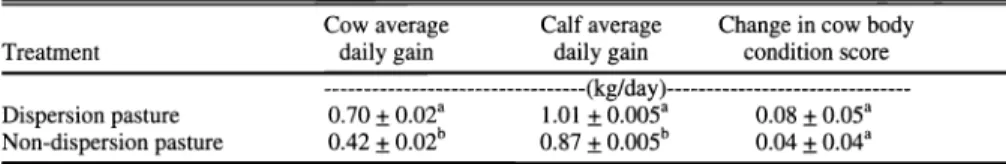
An analysis by treatment (dispersion ver- sus non-dispersion pastures) of the 2 years of data in cattle weight gains and changes in cow body condition scores were con- ducted using the SAS (SAS Institute 1990) general linear models procedure (Table 2).

Cattle provided off-stream water and salt did show improved weight gains ^(P <

0.01). Cows in dispersion pastures gained 0.27 kg/day more than cows without off- stream water and salt. There was no sig- nificant change in body condition scores for cows between treatments (P < 0.56).

Calves with off-stream water and salt gained on average 0.14 kg/day more than calves in non-dispersion pastures ^(P <

0.01). This translated into improved ani- mal performance that increased revenue received when cattle were sold.

Forage utilization in the riparian and upland portions of study pastures was esti- mated (Dickard 1998) using the Bureau of Land Management's utilization formula, shown in equation 22 (USDI 1996).

Production weights were sampled in the control and treatment pastures to derive the utilization estimate.

(control plot - treatment plot) I

control plot = % utilization (22) Data collected at the Hall Ranch suggest the ratio between riparian and upland uti- lization is influenced by off stream water and salt. [Utilization can be difficult to estimate (Burkhardt 1997). The method used here was on a total vegetation pro- duction basis. The utilization values listed here may not be "exact" but should be considered an indication of the riparian and upland utilization ratio that is achieved when the off-stream water and salt project is used.] When off-stream water and salt was provided, a larger per- centage of upland vegetation was grazed compared to riparian vegetation. If cattle have to be removed when utilization reaches 35% in the riparian area, more upland forage can be consumed before reaching this restriction if cattle are attracted out of the riparian area. The study shows only 25% of the upland for-

Table 2. Comparison by treatment of average daily gain (kg/day) for cattle and change in body condition scores for cows, 1996 and 1997.

Treatment

Cow average Calf average Change in cow body daily gain daily gain condition score ---(kg/day)--- Dispersion pasture 0.70 ± 0.02' 1.01 ± ^{0.005a 0.08} ± ^0.05a Non-dispersion pasture 0.42 ± 0.02b 0.87 ± ^{0.005b 0.04} ± ^0.04a

a,b

Means

standard errors) in the same column followed by different superscript significantly differ (P

JOURNAL OF RANGE MANAGEMENT 56(5) September 2003 421

Table 3. Riparian utilization standard and resulting upland utilization for public lands.

Nonproject Pastures (pi)

Project Pasture (p2) without Off-Stream

Water

Pasture (p2) with Off-Stream Water

Riparian Vegetation 0.35 0.35

Upland Vegetation 0.5 0.25

age in a non-project pasture will have been grazed when the 35% utilization level is reached in the riparian area. Table 3 lists the allowable utilization levels if the man- ager complies with the desired utilization limitations. Thus the a ^{in equation 20 is}

influenced by the use of the dispersion project as shown in equation 23 (non-dis- persion) and 24 (dispersion). More upland forage (g2) is consumed before reaching the limits of riparian utilization (g ¹⁾ in the dispersion pastures in equation 20.

OVERg1,t > 1.4 ^* OVERg2,t (23) OVERg1,t > 0.7 ^* OVERg2 _t (24) The assumption has been made that the cattle are grazing in the same distribution ratio between the riparian and upland throughout the grazing season. Based upon GIS analysis of distribution patterns, this appeared to be true for cattle in pas- tures with off-stream water and salt (Dickard 1998). In contrast, the non-dis- persion project pastures showed cattle concentrated in the riparian areas early in the grazing period and then moved more to the uplands in the latter parts of the grazing period.

Solution Method

The bioeconomic model is solved using the General Algebraic Modeling System (GAMS) developed by Brooke et al. using the GAMS/MINOS solver (Modular In- core Nonlinear Optimization System) developed by Murtagh and Saunders (Gill et al. 1992). A 60-year time horizon was chosen to allow the model to reach an equilibrium state and to capture the eco- nomic value of variables over the lifetime of the ranch. The equilibrium states of the model run with and without the dispersion project were compared to determine eco- nomic feasibility.

For simplification in the interpretation of the model results, the economic analy- sis of the dispersion impacts is run with a 7% discount rate. The 9 states of nature representing combinations of precipitation and market price conditions have been assigned numbers to simplify display of model results. The model number refers to the levels of crop year precipitation and cattle prices with 1= low, _{2 =} median and

3 = high. When a p ^is present, off-stream

water and salt are provided in the uplands of the summer pasture.

Results

The dispersion project has 3 significant impacts on annual gross margin. The first is the direct cost of the dispersion project.

The annual dispersion project costs are the sum of the investment cost spread over the lifetime of the equipment and the increas- es in variable costs such as labor. The sec- ond impact is the benefit of better cattle distribution. This allows more forage to be consumed in the uplands of pastures with off-stream water and salt before the ripari- an utilization limit is reached. This trans- lates into more animal units allowed to graze or fewer AVMs purchased from

other sources such as leased pasture and hay. The third impact is the increase in weight gain for cows and calves grazing in

pastures with the dispersion project.

Model results will be examined under 2

policy scenarios of with and without a riparian area utilization standard and over- grazing penalty. Comparison of those results should indicate the marginal effects on the long-term ranch operation.

Scenario A. Riparian Utilization Penalty

Scenario A assumes that there is a 35%

utilization limit on public land riparian areas. If utilization above this level occurs, a reduction in the ranch's permit is invoked for the next year. This penalty is set as a disincentive to exceed the utiliza- tion limit. Table 4 is a detailed presenta- tion of the number of cows stocked under each state of nature. Herd size fluctuates based on precipitation, price level and use of the dispersion project. Forage consump- tion also fluctuates with precipitation, price and use of the dispersion project as shown in Table 5. Private lease as a forage supply option is undertaken only when prices are in the median and high cate-

Table 4. Long run equilibrium number of cows for ranches operating with and without the disper- sion project under scenario A (penalty for exceeding 35% utilization of riparian vegetation on public lands) at 7% discount rate.

Precipitation

Dry Median Wet

Price Non-project Project Project

Low Median High

281 281

307 306

307 307

33 337

331

336 373

336 373

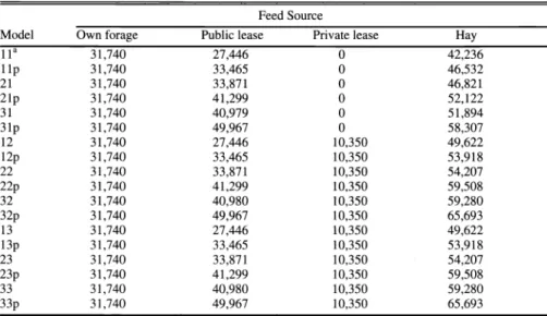
Table 5. Long run equilibrium decision levels for forage usage (in AUD) under scenario A (penalty for exceeding 35% utilization of riparian vegetation on public lands) at 7% discount rate.

Feed Source

Model Own forage Public lease lease

ila 31,740 27,446 0

lip

31,740 33,465 0

21

31,740 33,871 0

2lp

31,740 41,299 0

31

31,740 40,979

31p 31,740 49,967

12

31,740 27,446

12p

31,740 33,465

22

31,740 33,871

22p

31,740 41,299

32

31,740 40,980

32p

31,740 49,967

13

31,740 27,446

13p

31,740 33,465

23

31,740 33,871

23p

31,740 41,299

33

31,740 40,980

33p

31,740 49,967

aModel

number refers

crop year precipitation and prices, respectively, where 1= low,

median,

high and "p"

indicates the dispersion project.

422 JOURNAL OF RANGE MANAGEMENT 56(5) September 2003

gories. Herd size is reduced by approxi- mately 42 cows during low cattle prices rather than leasing the more expensive for- age. Under the condition of limiting ripari- an utilization to 35% on public lands and low cattle prices, the 300-cow ranch can- not support the herd if off-stream water and salt are not provided during median precipitation years. In all model versions, the maximum allowable level of forage is consumed from privately owned range, which is restricted regardless of precipita- tion conditions to

month of feed for 345 animal units. If all pastures had been allowed to fluctuate under the various crop year precipitation levels, herd size would have more dramatic decreases in dry years, remain constant in median years and higher increases in wet years. Under all price conditions, hay is fed only during the required 5 months of winter. The high- est allowable level of forage use, under desired riparian utilization levels, is con- sumed from the public lease. The maxi- mum value for public forage changes depends upon the precipitation conditions and the use of the dispersion project

(Table 4). For the median rain and price model, an extra 7,430 AUDs (or 240 AVMs) of forage consumption are sup- ported with improved distribution between riparian and upland areas. This yields enough forage to support an additional 34.5 animal units for 7 months.

In all states of nature, the dispersion project increases the ranch's average annual gross margin. Table 6 illustrates the change in average annual ranch gross

Table 6. Change in average annual gross mar- gin less dispersion costs when dispersion pro- ject is implemented under scenario A (penal- ty for exceeding 35% utilization of riparian vegetation on public lands) at 7% discount rate.

Precipitation

Price Dry Median

Low + $3,820 + $4,526 $5,303 Median + $6,595 ⁺ $7,289 $11,737 High + $9,327 + $11,075 $13,008

margin realized when cattle are provided off-stream water and salt during a month and half of summer grazing. Increases of

$3,800-$13,000 ^are found by implement- ing the dispersion project, depending upon precipitation and price conditions. Even in low price and drought conditions, the additional $3,800 in average annual gross margin indicates a rapid payback period for the project. Initial investment costs for the dispersion project are approximately

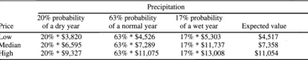
Table 7. Expected value for off-stream water and salt in terms of change in average annual gross margin under scenario A (penalty for exceeding 35% utilization of riparian vegetation on public hands) at 7% discount rate.

Precipitation

Price

20% probability of a dry year

probability 17% probability

of a normal year of a wet year value

Low 20% * _{$3,820 63%} *

*

Median 20%

$6,595 63%

17%

High 20%

$9,327 63%

17%

$2,400, which is spread over its useful life of 10 years.

An analysis of the increased $7,300 in average annual gross margin for the median price and precipitation state of nature shows approximately half ($3,800) ^is from the increased weight gain of cattle grazing in pastures with the dispersion project. The remaining amount of increase can be attrib- uted to the income from the sale of the extra 20 calves, 2 yearling heifers and ⁵ culled cows that are produced by the larger herd.

To compensate for the reality of imper- fect information, expected values were determined by assigning probabilities to the different states of nature. The crop year precipitation data has a normal distri- bution with a standard deviation of ⁶⁶ mm. The probability of precipitation being equal to or less than the low value is 20%.

The probability of rain being greater than or equal to the high value is 17%. This yields a 63% chance that the value will be near the median value (within plus or minus

standard deviation from the medi- an value). Cattle prices exhibit autocorre- lation because of their tendency to follow a trend in the price cycle. In other words, cattle prices do not generally jump from a low price in

year to a high price in the following year. Therefore, the probability of switching between low, median and high values is extremely low. To compen- sate for this fact, 3 expected values of the dispersion project, one for each price level, are calculated according to the prob- ability of the precipitation states.

Table 7 is the payoff matrix for the expected value of the off-stream water and salt project. During the period of low cat- tle prices which Oregon ranchers were facing during the study, the project has an expected value of $4,500 in increased annual gross margin less the annual cost of implementing the dispersion project. As cattle prices increase, the expected value increases to $7,400 and $11,100 for medi-

an and high prices.

Scenario B. Project on Own Pasture with no Penalty

The dispersion project's expected value can also be calculated for situations in which the rancher is allowed a higher uti- lization level. For example, many range managers graze their own riparian lands at a 50% utilization level. The model is mod- ified to reflect this type of situation to determine if the project would increase annual gross margin. The penalty in the forage equation of motion (eq. 17) is removed from the model and the allow- able utilization percentages are increased as shown in Table 2. Table 8 illustrates the calculated expected change in annual gross margin when the project is imple- mented under these conditions. The expected value of providing off-stream water and salt is $2,400, $3,300 and

$4,000 under low, median and high price levels, respectively. These increases in expected gross margin are created from the additional weight gain of the culled cows and sold calves.

Table 8. Expected value for off stream water and salt in terms of change in average annual gross margin less the dispersion project costs under scenario B (riparian utilization of vegetation set at 50% on public lands) at 7% discount rate. (Expected value determined by multiplying the change in gross margin for that state of nature by the probability of that precipitation state occurring).

Precipitation 20% probability

Price of a dry year

63% probability of a normal year

probability

of a wet year value

Low 20%

Median 20%

High 20%

$3,476

$3,191

63%

63%

$3,314

$4,109

17%

*

* _$3,699

$4,536

$3,312

$3,976

JOURNAL OF RANGE MANAGEMENT 56(5) September 2003 423

Conclusions

Regardless of precipitation and price conditions, the off-stream water source and salt dispersion project examined in this study has a positive net return for ranches dealing with riparian grazing con- cerns. Better distribution of cattle allows for more upland forage to be consumed before reaching desired riparian utilization levels. The cows and calves also show higher weight gains when given access to off-stream water and salt. As riparian uti- lization becomes more restrictive, provid- ing off-stream water and salt may be a way that traditional grazing levels can remain while environmental objectives (reduced livestock impacts in the riparian area) are also obtained. Part of the disper- sion returns comes from the assumption that riparian utilization is a key factor in determining when cattle are removed from public lease pastures. However, criticism about utilization as a management tool must be considered. First, the vegetation sampling for utilization analysis is often done after cattle are removed. This means that a rancher will not know until after the fact that riparian utilization has exceeded the standard. To avoid this, a rancher would have to dedicate additional labor to periodic sampling during the grazing sea- son. In addition, the correct method for utilization analysis is subject to debate (Oregon State University 1998). There will continue to be conflict between the ranching industry and public agencies if utilization becomes the "measuring stick"

for management.

There are indirect economic benefits of the dispersion project not captured by the model. The only captured economic val- ues are the increased weight gains of cull cows and calves and the increase in num- bers of sale animals over the non-project conditions. The weight gain on the brood cows (non-sale animals) can also be asso- ciated with the improved health of cows and better calving success rates (Hart et al.

1988). As riparian areas recover, they also can provide the rancher with higher quali- ty and quantity of forage (Elmore and Beschta 1987). More biological research needs to be conducted in riparian lands on the interaction of grazing levels and future forage production yields.

There are also social benefits that may have accrued from implementing off- stream water and salt in livestock pastures.

In addition to an economic assessment, 3 other focus areas were included in the dis- persion project study. They include ripari- an area assessment, biodiversity counts

and animal behavior and performance.

The initial ecological assessments collect- ed for the project are beginning to be determined and may show improvements in riparian area health. With a positive economic feasibility assessment complet- ed on the dispersion project, it opens the door for discussion with range managers on improving riparian grazing with a method that should be non-threatening to their livelihood. More interdisciplinary studies like the one conducted at the Hall Ranch in the summer of 1996 and 1997 are needed so that all ecological, economic and social aspects are included in finding a sustainable solution to grazing in riparian areas. Bioeconomic models such as the one presented here are a movement toward a better method of comparison when com- plex biological systems are involved.

Literature Cited

Armour, C.L., D.A. Duff, and W. Elmore.

1991. The effects of livestock grazing on riparian and stream ecosystems. Fisheries (16):7-11.

Burkhardt, J.W. 1997. Grazing utilization limits: an ineffective management tool.

Rangelands 19(3).

Dickard, M.L. 1998. Management strategies for improved cattle distribution and subse- quent riparian health. M.S. Thesis. Univ. of Idaho, Moscow, Ida.

Elmore, W. and R.L. Beschta.1987. Riparian areas: perceptions in management.

Rangelands 9(6):260-265.

Gill, P.E., W. Murray, B.A. Murtagh, M.A.

Saunders, and M.H. Wright. 1992.

GAMS/MINOS, Appendix D. In: A. Brooke, D. Kendrick and A. Meeraus (eds.) GAMS: a user's guide, ed 2.25. The Scientific Press, San Francisco, Calif.

Hart, R.H., J.W. Waggoner, Jr., T.G. Dunn, C.C. Kaltenbach, and L.D. Adams. 1988.

Optimal stocking rate for cow-calf enterpris- es on native range and complementary improved pastures. J. Range Manage.

41(5):435-441.

Kauffman, J.B. and W.C. Krueger. 1984.

Livestock impacts on riparian ecosystems and streamside management implications. J.

Range Manage. 37(5):430-437.

Nielsen, D.B. 1984. Economic factors to be considered in sagebrush/grassland manage- ment, pp. 1373-1386. In: Developing strate- gies for rangeland management: A report prepared by the Committee on Developing Strategies for Rangeland Management.

Westview Press. Boulder, Colo.

Oregon State University. 1998. Stubble height and utilization measurements: uses and mis- uses. Ore. State Univ. Agr. Exp. Sta. Bull.

682.

Pope III, C.A. and G.L. McBryde. 1984.

Optimal stocking of rangeland for livestock

production within a dynamic framework.

Western J. Agr.. Econ. 9(1)160-169.

SAS Institute, Inc. 1990. SAS/STAT user's guide, 6.12 ed. Cary, N.C.

Skovlin, J. 1984. Impacts on grazing on wet- land and riparian habitat: a review of our knowledge, p. 1001-1103. In: Developing strategies for rangeland management.

National Research Council. Westview Press, Boulder, Colo.

Sneva, F.A. and ^D.N. Hyder. 1962.

Forecasting range herbage production in eastern Oregon. Ore. State Univ. Agr. Exp.

Sta. Bull. No. 588, Corvallis, Ore.

Standiford, ^R.B. and R.E. Howitt. 1992.

Solving empirical bioeconomic models: a rangeland management application. Amer. J.

Agr. Econ. 74(2):421-433.

Torell, L.A., K.S. Lyon, and E.B. Godfrey.

1991. Long-run versus short-run planning horizons and the rangeland stocking rate decision. Amer. J. Agr. Econ. 73(3)795-807.

Turner, B., F. Obermiller, J. Tanaka, ^B.

Eleveld, B. Broderick, G. Delaney, R.

Mills, and J. ^{Williams. 1998.} Enterprise budget, 300 cow/calf, mountain region.

Oregon State Univ. Ext. Serv. EM 8686.

U.S. Department of the Interior (USDI).

1996. Utilization studies and residual mea- surements. Bureau of Land Manage.

BLMIRS/ST-96/004+1730.

Workman, J.P. 1986. Range Economics.

Macmillan Publishing Co., New York, N.Y.

424 JOURNAL OF RANGE MANAGEMENT 56(5) September 2003