Mixed Causal Noncausal AR Processes and the Modelling of Explosive Bubbles

Munich Personal RePEc Archive

Mixed Causal-Noncausal AR Processes

and the Modelling of Explosive Bubbles

Fries, Sébastien and Zakoian, Jean-Michel

ENSAE, CREST

September 2017

Online at

https://mpra.ub.uni-muenchen.de/86926/

Mixed Causal-Noncausal AR Processes and the Modelling of

Explosive Bubbles

Sébastien Fries∗_{and Jean-Michel Zakoian}†

Abstract

Noncausal autoregressive models with heavy-tailed errors generate locally explosive processes and therefore provide a natural framework for modelling bubbles in economic and financial time series. We investigate the probability properties of mixed causal-noncausal autoregressive processes, as-suming the errors follow a stable non-Gaussian distribution. Extending the study of the noncausal AR(1) model by Gouriéroux and Zakoian (2017), we show that the conditional distribution in direct time is lighter-tailed than the errors distribution, and we emphasize the presence of ARCH effects in a causal representation of the process. Under the assumption that the errors belong to the do-main of attraction of a stable distribution, we show that a causal AR representation with non-i.i.d. errors can be consistently estimated by classical least-squares. We derive a portmanteau test to check the validity of the estimated AR representation and propose a method based on extreme residuals clustering to determine whether the AR generating process is causal, noncausal or mixed. An empirical study on simulated and real data illustrates the potential usefulness of the results.

Keywords: Noncausal process, Stable process, Extreme clustering, Explosive bubble, Portmanteau test.

∗_{CREST and Paris-Saclay University. E-Mail: [email protected]}

†_{Jean-Michel Zakoian, CREST and University Lille 3. Address: CREST, 5 Avenue Henri Le Chatelier, 91120}

1

Introduction

In the analysis of prices of financial assets such as stocks, it is common to observe phases of locally explosive behaviours, together with heavy-tailed marginal distributions and volatility clustering. Such features seem incompatible with classical linear models (namely the class of autoregressive-moving average (ARMA) models) which rely on the second-order properties of a time series. On the other hand, nonlinear models such as ARCH or stochastic volatility models are designed to capture volatility clustering, not to produce locally explosive sample paths mimicking bubbles in financial markets. However, the dynamic limitations of ARMA models are reduced if noncausal components (i.e. AR or MA polynomials with roots inside the unit disk) are introduced. For instance, all-pass models1 are linear time series with nonlinear behaviours, in particular ARCH effects [see Breidt, Davis and Trindade (2001) and the references therein]. More recently, Gouriéroux and Zakoian (2017, GZ hereafter) showed that a simple noncausal AR(1) process with heavy-tailed errors is able to produce the typical nonlinear behaviours observed for the prices of financial assets.

Noncausal processes or random fields have been thoroughly studied in the statistical literature [Rosenblatt (2000), Andrews, Calder and Davis (2009)], and have been applied in various areas, including deconvolution of seismic signals [Wiggins (1978), Donoho (1981), Hsueh and Mendel (1985)], and analysis of astronomical data [Scargle (1981)]. Recent years have witnessed the emer-gence of a significant line of research on noncausal models in the econometric literature [see e.g., Lanne, Nyberg and Saarinen (2012), Lanne, Saikkonen (2011), Davis and Song (2012), Chen, Choi and Escanciano (2012), Hencic and Gouriéroux (2015), Velasco and Lobato (2015), Hecq, Lieb and Telg (2016, 2017a, 2017b), Cavaliere, Nielsen and Rahbek (2017)]. The distinction between causal and noncausal processes is only meaningful in a non-Gaussian framework, and the increasing inter-est in Mixed causal-noncausal AR processes (MAR) parallels the widespread use of non-Gaussian heavy-tailed processes in economic or financial applications. Besides, rational expectations models in economics have been shown to admit solutions with noncausal components when departing from the finite variance assumption (see Gouriéroux, Jasiak and Monfort (2016)).

One important reason for introducing noncausal components in AR processes is to provide a mechanism for generating financial bubbles. GZ showed that the sample paths of a stationary noncausal AR(1) process with heavy-tailed errors may have locally explosive phases. Other recent researches have focused on data generating processes that are able to produce explosive behaviours

1

All-pass are ARMA models in which all roots of the AR polynomial are reciprocal of the roots of the MA

and model bubbles in financial markets. For example Phillips , Wu and Yu (2011), Phillips , Shi and Yu (2015) and more recently, in a continuous time framework, Chen, Phillips and Yu (2017) investigated mildly explosive processes. Apart from the generation of bubbles, noncausal AR(1) processes with stable distributed errors exhibit surprising features such as a predictive distribution with lighter tails than the marginal distribution, a martingale property in the causal representation when the errors follow a Cauchy distribution, or the presence of GARCH effects. It is of interest to know whether these structural properties extend to higher-order models. Indeed, first-order models are clearly not sufficient to capture complex behaviours of economic series, such as the occurrence of locally explosive behaviours with different rates of explosion, or different types of asymmetries in the growth and downturn phases of the bubbles.

The aim of this paper is to analyze the class of mixed causal-noncausal AR processes with heavy-tailed errors. The probability structure is studied under the assumption that the errors follow stable non-Gaussian distributions. Properties of the Least-Squares (LS) estimator are derived under the less stringent assumption that the noise distribution is in the domain of attraction of a non-Gaussian stable law. The paper is organised as follows. Section 2 studies the sample paths and the marginal distribution of MAR processes with stable errors. Sections 3 analyzes the conditional distributions through conditional moments. Conditional heteroscedasticity effects are depicted and causal representations are exhibited. Section 4 derives the asymptotic properties of LS estimator, deduces a portmanteau test, and studies identification of the strong representation based on the analysis of extreme residuals clustering. Sections 5 and 6 propose numerical illustrations based on simulated and real data, respectively. Section 7 concludes. Proofs are collected in the Appendix. Complementary results are provided in a Supplementary file.

2

Stable MAR(

p, q

) processes

MAR processes have been considered, among others, by Lanne and Saikkonen (2011), Gouriéroux and Jasiak (2016), Hecq, Issler, and Telg (2017).2 A MAR(p, q) process (Xt) is the strictly

station-ary solution of the difference equation

ψ(F)φ(B)Xt=εt, where ψ(F) = 1− p

X

i=1

ψiFi, φ(B) = 1− q

X

i=1

φiBi, (2.1) 2

See the latter reference for additional motivations on the use of MAR processes in time series econometrics. The

B and F are the usual lag and forward operators (BkXt=Xt−k, FkXt=Xt+k, k∈Z), (εt) is an

independent and identically distributed (i.i.d.) sequence, the polynomials ψ and φ have all their roots outside the unit circle and are such that ψp 6= 0 and φq6= 0. When q= 0 (resp. p= 0), the

model is called purely noncausal (resp. causal).

We assume that the errors εt follow a stable non-Gaussian distribution but the assumption will

be relaxed for the statistical inference. The generality and convenience of this class of distributions is now well established.3 Stable laws are easily characterised through their characteristic function:

εtis said to follow a stable distribution with parametersα∈]0,2[, β∈[−1,1], σ >0,µ∈R, denoted

εt∼ S(α, β, σ, µ), if

∀s∈R, E(eisεt_{) = exp}n_−σα_|s|α_{(1−i βsign(s)w(α, s)) +isµ}o_{, (2.2)}

where w(α, s) = tg πα₂

, if α 6= 1, and w(1, s) = −_π2ln|s|, otherwise. A stable random variable

X has regularly varying tails in the sense that P_{(X < −x) ∼ cα(1−β)x}−α _and P_{(X > x) ∼}

cα(1 +β)x−α asx→ ∞, withcα>0 andβ ∈(−1,1).

2.1 Sample paths

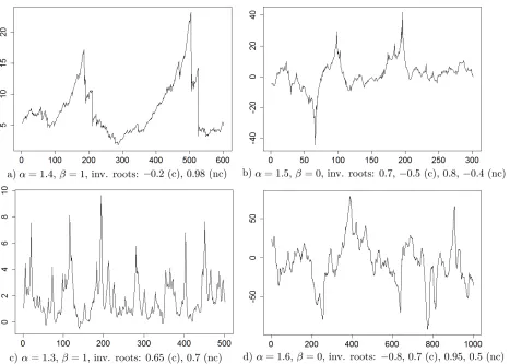
Examples of trajectories of four noncausal MAR processes are displayed in Figure 1. It can be seen that the trajectories feature locally explosive trends which are suited for the modelling of bubbles and positive feedback loop phenomena. Bubbles can be trending either upward or downward depending on the value of β. Whenβ = 1, the density of the errors is maximally skewed towards positive values, yielding trajectories like (a) and (c) which could be suited to model prices or volatilities. In particular, trajectory (a) displays bubble patterns similar to those of real prices (see for instance Figure 4 below). The influence of a smaller tail parameterαis visible when comparing trajectories (c) and (d): the extreme events of the former (α= 1.3) are more recurrent and further away from the central values than those of the latter (α= 1.6).

3

See for instance Embrechts, Klüppelberg, and Mikosch (1997), Samorodnitsky and Taqqu (1994) for the main

properties of stable distributions. A major justification for using stable distributions rather than other classes of

heavy-tailed distributions (such as the Student’st, the hyperbolic distributions) is that they are the only possible

limit distributions for properly normalized and centered sums of i.i.d. random variables (giving rise to generalized

Central Limit Theorems). Moreover, they are sufficiently flexible to accommodate asymmetry as well as fat tails.

Figure 1: Examples of trajectories of MAR(1,1) (left panel) and MAR(2,2) (right panel) processes with different parameters (nc: inverse of noncausal roots; c: inverse of causal root).

Under the assumptions made on the AR polynomial, (Xt) admits an MA(∞) representation4

Xt= +∞

X

k=−∞

dkεt+k. (2.3)

A simple index change Xt =

X

τ∈Z

ετdτ−t allows to interpret the sample path of Xt as a linear

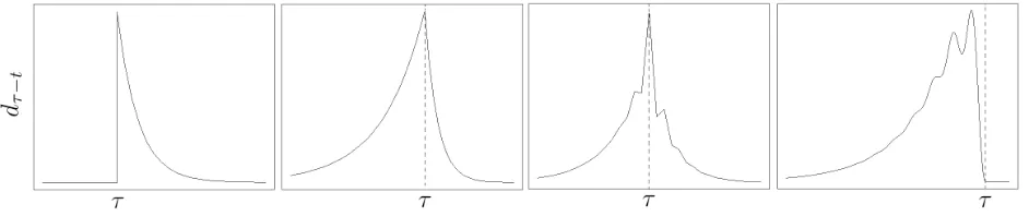
combination of baseline paths, t 7−→ dτ−t, weighted by stochastic i.i.d. coefficients ετ. Figure

2 depicts such baseline paths for four different MAR processes. The first panel illustrates the well-known impulse response function of a classical causal AR(1). The second panel displays an explosive exponential trend followed by a downward, faster decay and corresponds to the baseline path of a MAR(1,1) process. The remaining panels show more complex trajectories: the third one depicts the baseline path of a MAR(2,2) with dented upward and downward trends whereas the

4

It follows from Proposition 13.3.1 in Brockwell and Davis (1991) that the infinite sum in (2.3) is well defined

last one, corresponding to a noncausal AR(4) with two real and two conjugated complex roots, shows an upward trend with oscillations of increasing amplitudes and fixed pseudo-periods.

Figure 2: Examples of baseline paths t7−→dτ−t of MAR processes with characteristic polynomials, from left to

right: 1−0.7B ; (1−0.9F)(1−0.7B) ; (1−0.8F)(1 + 0.4F)(1−0.7B)(1 + 0.5B) ;

(1−0.99F)(1−965F)(1−0.98ei0.045πF)(1−0.98e−i0.045πF).

2.2 Marginal distribution

Our first result characterises the marginal distribution of the stable MAR(p, q).

Proposition 2.1 Let (Xt) the strictly stationary solution of the MAR(p, q) Model (2.1)where the roots of the polynomials ψ and φ are outside the unit disk and εt ∼ S(α, β, σ, µ). Then Xt has a stable stationary distribution, Xt∼ S(˜α,β,˜ σ,˜ µ˜) where

˜

α=α, β˜=β

P+∞

k=−∞|dk|αsign(dk)

P+∞

k=−∞|dk|α

,

˜

σ=σ





+∞

X

k=−∞

|dk|α



 1 α

, µ˜= µ

φ(1)ψ(1)−1{α=1} 2

πβσ

+∞

X

k=−∞

dkln|dk|.

It is worth noting that the tail indexα ofXtis that of the error term. In particular,E|Xt|s<+∞

fors < αand E_|Xt|α_{= +∞.}

3

Predictive distributions

In the presence of a noncausal component in the AR polynomial, the predictive density of a future observation given a sample of consecutive observations is generally not available in closed form. We start by showing that the Markov property holds whatever the errors distribution.

In the rest of the section, we will derive properties of the conditional distribution ofXtin direct time

when the errors are stable-distributed. We will focus on (i) the existence of conditional moments; (ii) explicit derivation of predictive formulas forXt; and (iii) the presence of ARCH effects in the

case of the MAR(1,q) process. More specific results will be detailed for the MAR(1,1) process.

3.1 Existence of moments of the conditional distribution

It follows from Proposition 2.1 that E_|Xt|s _{= ∞ for s ≥ α. The next result shows a different}

behaviour for the conditional moments, generalising the result obtained for the AR(1) by GZ.

Theorem 3.1 If (Xt) is the MAR(p, q) solution of Model (2.1) withεt∼ S(α, β, σ, µ), we have

E_[|Xt|γ_{|Xt−1, Xt−2, . . .]<∞, a.s., whenever 0< γ <2α+ 1.}

The conditional distribution in direct time, that is with respect to the past observations, thus has lighter tails than both the marginal distribution and the distribution conditional on the future. In particular, whatever the heaviness of the tails ofεt, the conditional expectation ofXtalways exists.

The conditional variance in direct time also exists provided that the tails of the errors distribution are not too fat (α >1/2).5

3.2 Prediction of future values for the MAR(1, q) processes.

Prediction at any horizon can be fully characterised for the symmetric MAR(1, q) process. The next proposition extends in a non trivial way the prediction formula obtained by GZ for the noncausal AR(1), i.e. for the MAR(1,0). LetF_{t =σ(Xt, Xt−1, . . .) the canonical filtration of process (Xt).}

Forx6= 0 and r∈R_{, let x}<r> _{= sign(x)|x|}r_.

Proposition 3.2 Let the MAR(1, q) process(1−ψF)φ(B)Xt=εt, under the assumptions of Model

(2.1), with εt ∼ S(α,0, σ,0). Then there exists for any h ≥ 0 a polynomial Ph of degree q such that

E_[Xt+h|F_{t−1] =}P_h(B)Xt−1.

Forh= 0, the above formula holds with

P_{0(B)Xt−1 =ψ}<α−1>_{Xt−1+ (1−ψ}<α−1>_{B)(φ1Xt−1+. . .+φqXt−q),} 5

A discrepancy between conditions of existence for marginal and conditional moments also holds for many nonlinear

causal models: for instance GARCH (see e.g. Francq and Zakoian (2011), Chapter 2), or models for time series of

and we have the semi-strong causal representation

(1−ψ<α−1>B)φ(B)Xt=ηt, (3.1) withE_[ηt|F_{t−1] = 0.}

The proof is based on: i) disentangling pure causal and noncausal components of the MAR process (in the spirit of Lanne and Saikkonen (2011), Gouriéroux and Jasiak (2016)); ii) using the closed-form expression of the conditional expectation of the pure noncausal component, and (iii) invoking the Markov property.6

It is worth noting that the conditional expectation is linear in the past and can be explicitly computed. By comparison with finite variance AR processes, the semi-strong representation (3.1) is surprising. Indeed, in theL2_{framework, if (X}

t) is mixed causal-noncausal satisfyingψ(F)φ(B)Xt=

εt,then there exists a causal version of (Xt) given byψ(B)φ(B)Xt=Zt,where (Zt) is uncorrelated

with zero mean and finite variance (see for instance Brockwell and Davis (1991), Section 4.4).7 In our framework, the noncausal component (1−ψF), with |ψ|< 1, is transformed into the causal component (1−ψ<α−1>_B).

In the Cauchy case (α= 1) we get, when ψ >0,

Eh_Xt Ft−1

i

=Xt−1+ (1−B)(φ1Xt−1+. . .+φqXt−q), (3.2)

with by convention φ1 = . . . = φq = 0 when q = 0. Hence, the martingale property established

by GZ (Proposition 3.3),E

XtF_t−1

=Xt−1, only holds for the noncausal AR(1) (i.e. whenq= 0).

The asymptotic behaviour of the conditional expectation -when the horizonhtends to infinity-is highly dependent on the tail indexα. Proposition 3.2 allows us to distinguish different behaviours summarised in the following Corollary.

Corollary 3.1 Under the assumptions of Proposition 3.2, we have almost surely

E[Xt+h|Ft−1] −→

h→∞

  

 

0 if α∈(1,2), ℓt−1 if α= 1, 6

The inherent complexity of the pure noncausal component whenp >1, for which no such closed-form expression

exists, does not allow us to go beyondp= 1 for the results of this section. 7

The equalityψ(F)Zt=ψ(B)εtindeed implies that (Zt) has a spectral density given byfZ(λ) =σ

2

2π

|ψ(e−iλ_)|2

|ψ(eiλ_)|2 =

σ2

2π

whereσ2_{= Var(ε}

where ℓt−1 is an Ft−1-measurable random variable. Moreover, when α∈(0,1) and q= 1,

E[Xt+h|Ft−1] −→

h→∞∞.

Ifα∈(1,2), that is for lighter tails within the stable family, the conditional expectation always tends to 0 which is the unconditional expectation. This is consistent with the L2 _framework

(Brockwell and Davis (1991), p.189). For α= 1, the absolute value of the conditional expectation tends to a finite limit whereas the unconditional expectation does not exist. The general case when

α∈(0,1) is more intricate and is detailed in the Supplementary file.

3.3 Conditional heteroskedasticity of the Cauchy MAR(1, q)

All-pass models are well known examples of strong linear models displaying ARCH effects (namely the correlation of the squares). However, such effects are difficult to characterise without an explicit specification of the errors specification. The following result provides an explicit characterization of ARCH effects through the conditional variance of MAR processes with Cauchy innovation, extending again the results obtained by GZ for the noncausal AR(1).

Proposition 3.3 Let Xt be a MAR(1, q) process (1−ψF)φ(B)Xt = εt with εt i.i.d.∼ S(1,0, σ,0). Then, for any h≥0, there exists a polynomial Qh(z) =Phi=0qi,hzi such that

V_Xt+h Ft−1

=

(φ(B)Xt−1)2+

σ2

(1− |ψ|)2

ch−

Qh(sign ψ)

2

,

withch =Phi=0

Ph

j=0qi,hqj,h(sign ψ)i+j|ψ|−min(i,j)−1.

Polynomials Qh(z), for h ≥ 0, are defined in the Appendix. The causal representation (3.1) can

then be completed and reveals quadratic ARCH effects in the Cauchy MAR(1, q) process.

Corollary 3.2 Under the assumptions of Proposition 3.3, there exists a sequence (ηt) of random variables such that,

(1−sign(ψ)B)φ(B)Xt=σtηt,

σ2_t =

₁

|ψ|−1

(Xt−1−φ1Xt−2−. . .−φqXt−q−1)2+

σ2

|ψ|(1− |ψ|).

where E_[ηt|F_{t−1] = 0,}E

η_t2 F_t−1

= 1.

The process et = σtηt is however not a ARCH in the strict sense: first, because the errors ηt

are not i.i.d., and second, because the volatility is a function of the Xt−i (not of the et−i). This

3.4 The MAR(1,1) process.

The results of this section can be made completely explicit for the MAR(1,1) model defined by

(1−ψF)(1−φB)Xt=εt, with εti.i.d.∼ S(α, β, σ, µ), (3.3)

with |φ| < 1 and 0 < |ψ|< 1. The coefficients of the MA(∞) representation (2.3) are given by:

dk=

ψk

1−φψ, for anyk≥0, anddk= φ−k

1−φψ, for anyk≤0. Then Xt∼ S

α,β,˜ σ,˜ µ˜ with

˜

β =β

_{1−sign(φ)|φψ|}α

1− |φψ|α

1−sign(ψ)|ψ|α

1− |ψ|α

1−sign(φ)|φ|α

1− |φ|α

,

˜

σ = σ 1−φψ

_{1− |φψ|}α

(1− |ψ|α_{)(1− |φ|}α₎

1_α

,

˜

µ= µ

(1−ψ)(1−φ) −1{α=1}

2βσ π(1−φψ)

_ψln|ψ|

(1−ψ)2 +

φln|φ|

(1−φ)2 −

(1−φψ) ln|1−φψ|

(1−ψ)(1−φ)

.

In particular, whenψ, φ >0 and the errors are Cauchy distributed, that is whenεti.i.d.∼ S(1,0, σ,0),

then the above formulae simplify and Xt∼ S

1,0, σ

(1−ψ)(1−φ),0

.

We now derive an explicit prediction formula for the MAR(1,1) process whenβ =µ= 0. Proposi-tion 3.2 yields for anyh≥0,

Eh_Xt+h Ft−1

i

=φh+1Xt−1+ (Xt−1−φXt−2)(ψ<α−1>)h+1 h

X

i=0

(φψ<1−α>i,

=       

φh+1_X t−1+

(ψ<α−1>)h+1−φh+1

1−φψ<1−α> (Xt−1−φXt−2), if φψ<1−α> 6= 1,

φh+1[Xt−1+ (h+ 1)(Xt−1−φXt−2)], if φψ<1−α> = 1.

Whenψ >0 andα= 1, Corollary 3.2 yields

(1−B)(1−φB)Xt=ηt

s

(ψ−1_−1)(X

t−1−φXt−2)2+

σ2

ψ(1−ψ), whereE_[ηt|F_{t−1] = 0 and} E

η2 t

F_t−1

= 1. The conditional variance at horizonh in Proposition 3.3 takes the more explicit form, for anyh≥0,

V_Xt+h Ft−1

=



c_h−

1−φh+1

1−φ

!2



(Xt−1−φXt−2)2+

σ2

(1−ψ)2

,

where

ch =

(1 +φψ)ψ−h−1

(1−φψ)(1−φ2_ψ) −

2φh+1

(1−φ)(1−φψ) +

(1 +φ)φ2(h+1)

4

Statistical Inference

This section is devoted to the LS estimation of the MAR(p, q) model

ψ0(F)φ0(B)Xt=εt, (4.1)

whereψ0(z) = 1−Ppi=1ψ0izi, φ0(z) = 1−Pqi=1φ0izi, withψ0(z)= 0 and6 φ0(z)6= 0 for|z| ≤1.

Contrary to other estimation methods such as Maximum Likelihood (ML)8, LS do not require full specification of the errors distribution. We relax the assumption that (εt) is anα-stable sequence

and rather assume that the law ofεt belongs to the domain of attraction of a stable distribution.

Specifically, we assume that there exists a functionL which is slowly varying at infinity9 such that

P_{(|ε0|> x) =x}−α_{L(x), and lim}

x→∞

P_{(ε0 > x)}

P_{(|ε0|> x)} →c∈[0,1]. (4.2)

This more general assumption on the errors distribution encompasses in particular the fully para-metric α-stable framework under which the properties of the previous section were derived. Re-placingα-stable laws by their domain of attraction alleviates the risk of misspecification.10

We will first derive the asymptotic properties of estimators of a "all-pass causal representation" of the MAR(p, q) process. Then, we will develop a portmanteau test for checking the validity of the estimated representation. Finally, we will consider selecting the true model, among the different specifications admitting the same all-pass representation, based on properties of extreme clustering.

4.1 All-pass causal representation

A difficulty in the inference of mixed causal-noncausal AR processes, is that many representations with seemingly uncorrelated errors hold. Breidt, Davis and Trindade (Section 4.3, 2001) showed that if (Xt) is the strictly stationary solution of Model (4.1)-(4.2), then for any polynomial η∗0(z)

obtained fromψ0(z)φ0(z) by replacing one or several roots by their inverses, we have

η₀∗(B)Xt=ζt∗, (4.3) 8

See Andrews, Calder and Davis (2009) for asymptotic properties of the ML estimator of both causal and noncausal

AR processes with non-Gaussianα-stable distribution. In the finite variance setting, ML estimation of MAR models

based on Student’stdistribution was studied by Hecq et al. (2016). 9

i.e. limx→∞L(tx)/L(x) = 1,∀t >0.

10

The same assumption was considered in the context of causal AR processes for the study least-absolute deviation

where (ζ_t∗) is an all-pass process.11 Such representations (4.3) will be called all-pass in the following. In the set of all-pass representations, one is characterized by a polynomial η0 having all its roots

outside the unit disk

η0(B)Xt=ζt, where η0(B) =ψ0(B)φ0(B) = 1− p+q

X

i=1

η0iBi, (4.4)

and (ζt) is an all-pass process. In the sequel, we call (4.4) theall-pass causalrepresentation of (Xt).

Now, let ρ(h) = P∞

k=−∞dkdk−h/ P∞k=−∞d2k

for h ∈ Z_{, where the dk’s are the MA(∞)}

coefficients in (2.3).

Proposition 4.1 Let (Xt) be the strictly stationary solution of model (4.1) under (4.2). Then, the ρ(h)’s satisfy the recursion

ρ(h) =

p+q

X

i=1

η0iρ(h−i), ∀h >0, (4.5) where the coefficients η0i are obtained from (4.4).

It is worth noting that, although the autocorrelations of Xt do not exist, the empirical

autocorre-lations can be computed and converge to the coefficientsρ(h), which satisfy the usual Yule-Walker equations. Such equations explain why the coefficients of the all-pass causal representation of (Xt)

can be consistently estimated by LS.

4.2 Least-squares estimation

We consider LS parameter estimation of the all-pass causal representation (4.4), based on observa-tionsX1, . . . , Xn of the MAR(p, q) model (4.1). A LS estimator of η0= (η01, . . . , η0,p+q)′ is

ˆ

η= arg min

η∈Rp+q

L∗_n(η), (4.6) where

L∗_n(η) =

n

X

t=p+q+1

Xt− p+q

X

i=1

ηiXt−i

!2

. (4.7)

For h ≥ 0, let ˆγ(h) = Pn−h

t=0 XtXt+h and denote ˆρ(h) = ˆγ(h)/ˆγ(0) the mean-unadjusted sample

autocorrelation of order h. The LS estimator of η₀ coincides, up to negligible terms, with the Yule-Walker estimator and is given by

ˆ

η= ˆΓ−_n1γˆ_n, Γˆn= [ˆγ(i−j)]i,j=1,...,p+q, γˆn= [ˆγ(i)]i=1,...,p+q. (4.8) 11

When the second-order moments are finite, all-pass processes are uncorrelated. Andrews and Davis (2013)

showed that this property continues to hold "empirically" in the infinite variance case, in the sense that the sample

Proposition 4.2 Let (Xt) be the strictly stationary solution of model (4.1)-(4.2). Then the LS estimator ηˆ is consistent: ηˆ →η₀ in probability, asn→ ∞.

To derive the asymptotic distribution of the LS estimator ofη₀, we introduce the sequences

an= inf{x:P(|ε0|> x)≤n−1}, and a˜n= inf{x:P(|ε0ε1|> x)≤n−1}, (4.9)

defined by Davis and Resnik (1986). Let J the (p+q)×(p+q) shift matrix, with ones on the superdiagonal and zeros elsewhere. Forℓ= 1, . . . , p+q letK(ℓ)=Jℓ+tJℓ (withK(p+q)=0). Let

L= [K K(2) . . . K(p+q)]. We start by providing the asymptotic behaviour of the LS estimator under the simplifying assumption that the distribution ofεt is symmetric. This assumption will be

relaxed in the next section. The following result is a consequence of Davis and Resnik (1986).

Proposition 4.3 Let (Xt) be the strictly stationary solution of Model (4.1) with symmetric i.i.d. errors (εt) satisfying (4.2) and E|εt|α =∞.

Then, letting ρ= [ρ(i)]i=1,...,p+q,R= [ρ(i−j)]i,j=1,...,p+q,

a2_n

˜

an

(ˆη−η₀)→d R−1{I_p+q−L(I_p+q⊗R−1ρ)}Z, where Z= (Z1, . . . , Zp+q)′, (4.10)

Zk = P+_l=1∞{ρ(k+l) +ρ(k−l)−2ρ(l)ρ(k)}Sl/S0, for k = 1, . . . , p+q, and S0, S1, S2, . . . are

independent stable random variables;S0 is positive with index α/2 and Sj, for j≥1, has index α. If the law of |εt| is asymptotically equivalent to a Pareto, (4.10) holds witha2n/˜an= (n/lnn)1/α.

The α-stable domain of attraction assumption on (εt) impacts the asymptotic behaviour of the

LS estimator in two important aspects: ι) the limiting distribution depends on α and ιι) the convergence rate is a2n

˜ an ∼ n

1/α_{L˜(n), for some slowly varying function ˜L (see p.551, Davis and}

Resnick, 1986). RequiringE_|εt|α _{=∞ ensures that the law ofε0ε1 belongs to theα-stable domain}

of attraction (see Cline (1983), Theorem 3.3 iv) p. 80).

Example 4.1 (MAR(1,1) process (continued)) For the MAR(1,1) process, Proposition 4.3 allows to compute the asymptotic distribution of the LS estimator of (φ0+ψ0, φ0ψ0), using

R−1{I2−L(I2⊗R−1ρ)}=

1 +φ0ψ0

(1−ψ2

0)(1−φ20)



 

(1 +ψ0φ0)2+ (ψ0+φ0)2 −(ψ0+φ0)

−2(ψ0+φ0)(1 +ψ0φ0) 1 +ψ0φ0



 .

This matrix can be straightforwardly estimated by plugging LS estimators of φ0+ψ0 and φ0ψ0.

by r1 < r2 the inverses of the roots of η0(z) (thus ri ∈ {φ0, ψ0} for i = 1,2), that is (r1, r2) =

η01−

q

η2

01+ 4η02, η01+

q

η2

01+ 4η02

/2 := f(η01, η02). By the delta method, an asymptotic

confidence region can be deduced for (r1, r2): letRn,α such thatP[(r1, r2)∈ Rn,α] = 1−α. Thus,

P[{(φ0, ψ0),(ψ0, φ0)} ⊂ Rn,α] = 1−α.Finally, lettingR∗n,α the symmetric of Rn,α around the line

r1 =r2, we get an asymptotic confidence region for (φ0, ψ0): P[(φ0, ψ0)∈ Rn,α∪ R∗n,α]≥1−α.

The knowledge of index α is not required for the computation of the LS estimator, but the asymptotic distribution, as well as the normalizing constantsanand ˜an, depend onα. The presence

of this nuisance parameter renders inference difficult for this class of model. Having estimated the AR coefficients, one could overcome this hurdle by using a standard estimator for the tail indexα. For instance, for a random sample (X1, . . . , Xn), the so-called Hill (1975) estimator of 1/αbased

onm+ 1 upper order statistics is defined as: ˆ

α−_m1= 1

m

m

X

i=1

log X(i)

X_(m+1)

!

,

where X_(i) > 0 is the ith order statistic in decreasing order (X₍₁₎ ≥ X₍₂₎ ≥ . . . X_(n)). Mason (1982) proved that the Hill estimator is a consistent estimator of 1/α, provided n→ ∞, m→ ∞

and m/n → 0, in the case of i.i.d. variables. Consistency and asymptotic normality under serial dependence conditions - including ℓ-dependence, β-mixing, ARCH - were established by various authors (see e.g. Hill (2010), De Hann et al. (2016) and the references therein). An alternative to the estimation of the asymptotic distribution is to base inference on bootstrap. Recently Cavaliere, Nielsen and Rahbek (2018) proposed bootstrap schemes for noncausal AR models with infinite variance, and showed their usefulness for hypothesis testing. Extension of this approach to mixed AR models remains an open issue.

4.3 Relaxing the symmetry assumption

In the previous section, we derived the asymptotic behaviour of the LS estimator ofη0 assuming

the errors (εt) were symmetrically distributed. We here relax the symmetry assumption and only

require (εt) to satisfy (4.2). The asymptotic behaviour of the LS estimator remains unchanged in

the case 0< α <1, and holds for 1< α <2 after a mean-adjustment.12 Let ˜γ(h) = Pn−h

t=0(Xt−X¯)(Xt+h−X¯) where ¯X = 1/nPnt=0Xt, and denote ˜ρ(h) = ˜γ(h)/γ˜(0) 12

A bias term appears in the caseα= 1 when departing from the symmetry assumption (See Davis and Resnik

the mean-adjusted sample autocorrelation of orderh. Similarly to (4.8), define the mean-adjusted Yule-Walker estimator ˜η by

˜

η= ˜Γ−_n1γ˜_n, Γ˜n= [˜γ(i−j)]i,j=1,...,p+q, γ˜n= [˜γ(i)]i=1,...,p+q. (4.11)

Proposition 4.4 Let (Xt) be the strictly stationary solution of Model (4.1), where(εt) is an i.i.d. sequence satisfying (4.2)and E|εt|α =∞.

• If 0< α <1, then (4.10) holds.

• If 1< α <2, then (4.10) holds withηˆ replaced by the mean-adjusted estimatorη˜.

4.4 Diagnostic checking

Validity of the estimated model can be assessed by studying the sample autocorrelations of the residuals. Once the parameters of the all-pass representation (4.4) have been estimated by LS, with ˆη= (ˆηi)i=1,...,p+q, the corresponding residuals are defined by

ˆ

ζt=Xt− p+q

X

i=1

ˆ

ηiXt−i, t=p+q+ 1, . . . , n. (4.12)

Let, for h≥0, ˆρ_ζˆ(h) = ˆρ_ζˆ(−h) = ˆ γˆ_ζ(h)

ˆ

γ_ζˆ(0) where ˆγζˆ(h) = Pn

t=h+p+q+1ζˆtζˆt−h and ˆγ_ζˆ(−h) = ˆγ_ζˆ(h). For

a fixed integerH ≥1, let ˆρ_ζˆ= [ˆρ_ζˆ(1), . . . ,ρˆ_ζˆ(H)]′.

Proposition 4.5 Under the assumptions of Proposition 4.3, the vector of residuals empirical au-tocorrelations satisfies

a2_n

˜

an

ˆ

ρ_ζˆ−→d γ(0)AHZ, where Z= (Z1, . . . , ZH+p+q)′, whereγ(0) =P∞

k=−∞d2k, theZi’s are as in Proposition 4.3, andAH is a non randomH×(p+q+H) matrix function of the sole AR coefficients (not of the errors distribution).

Details regarding matrix AH are available in the proof. Note that the symmetry assumption

can be relaxed as in Section 4.3. It is now possible to propose a portmanteau test to check for residuals autocorrelations based for instance on the statistic

TH =a2n˜a−n1 H

X

i=1

|ρˆ_ζˆ(i)| −→d

n→+∞kγ(0)AHZk1, (4.13) with kxk1 =P|xi| for any vector x = (xi). Practical implementation of the test finally requires

4.5 Model selection based on extremes clustering

The all-pass causal representation (4.4) is compatible with all MAR(p′, q′) models of the form (4.3) (with p′_+q′ _{= p+q). Such models could have generated the observations, and it is important} to detect which one is the true model. A distinctive feature of the latter is that the errors are i.i.d., not only "asymptotically empirically non-autocorrelated" as in (4.3) (see footnote11_{). Having}

estimated the coefficients of the polynomial η0, a natural strategy for assessing the validity of a

candidate model, with polynomial η∗

0, is to test the independence of the ζt∗ in (4.3). We propose

an approach based on extreme clustering of the residuals.13

4.5.1 Point process of exceedances

This dependence materialises here in an important feature known as extreme clustering (see e.g. Hsing, Hüsler, Leadbetter (1988), Markovich (2014) and Chavez-Demoulin and Davison (2012) for a literature review) which yields a way to identify the strong representation among the all-pass alternatives. Let us introduce a linear process (Yt) with two-sided MA(∞) representation

Yt = Pk∈Zckεt+k, where (εt) is an i.i.d. sequence satisfying (4.2), Pk∈Z|ck|s < +∞ for some

0 < s < α, s ≤ 1, and assume max|ck|= 1 for convenience. In our context, Yt will typically be

substituted for the errors εt of the strong representation and the errors ζt∗ of competing all-pass

representations.

We can study the time indices for which a−_n1Yk falls outside the interval (−x, x), for x >0. The

corresponding point process converges as the number of observationsngrows to infinity (see Davis and Resnick (Section 3.D, 1985)):

n

X

k=1

δ_(k/n,a−1 n Yk)

· ∩Bx

_d

−→

+∞

X

k=1

ξkδΓk, (4.14)

whereδ is the Dirac measure,Bx = (0,+∞)×

(−∞,−x)∪(x,+∞),{Γk, k≥1}are the points of

a homogeneous Poisson Random Measure (PRM) on (0,+∞) with rate x−α_,14 _{and ξ}

k= Card{i∈ 13

Alternative approaches based on non-parametric and rank-based tests have been proposed for testing iid-ness of

innovations (see for instance Brock, Dechert, LeBaron and Scheinkman (1996), and Duchesne, Ghoudi and Rémillard

(2012)). However, the validity of these tests requires to have√n-consistent estimators of the model parameters,

which is not the case in theα-domain of attraction framework as shown in Proposition 4.3. 14

See Daley and Vere-Jones (2007): {Γk, k≥1}are the points of a homogeneous PRM on (0,+∞) with ratex−α

Z_{:Jk|ci|>1}where{Jk, k≥1}are i.i.d. on (1,+∞), independent of{Γk}, with common density:}

f(z) =αz−α−1_1(1,+∞)(z). (4.15) The sequences{Γk}and{ξk}are interpreted (see for instance Leadbetter and Nandagopalan (1989))

as describing respectively the occurrence dates of clusters of extreme events and the size of these clusters (i.e. the number of co-occurring extreme events). We will now outline the interest of analysing extreme events for model selection.

4.5.2 Analysing the error processes of competing models

Let (Xt) be the MAR(p, q) strictly stationary solution of Model (4.2)-(4.1) and assume the order

p+q and the roots of η0 are known. There is a finite number of competing representations among

which the strong one lies. Denoting (εt) of the errors of the strong representation and generically

(ζ_t∗) the errors of any specific all-pass representation, we can analyse their extreme clustering behaviour using (4.14).

Error process of the strong representation The i.i.d. errors (εt) of the strong representation

admit the trivial MA form εt=Pk∈Zckεt+k with c0 = 1 and ck= 0 fork6= 0. Thus, substituting

Yt for εt, (4.14) holds with ξk = Card{i∈ Z :Jk|ci|> 1} = 1{Jk>1} = 1. The random variables

(ξk) describing the size of the cluster of extremes are degenerate in this case: the extreme errors

(εt) tend to appear isolated from each other.

Error process of an all-pass representation The (rescaled) errorsζ∗

t of an all-pass

represen-tation always admit an infinite one-sided or two-sided MA form, sayζ_t∗ = P

k∈Z ck

maxj|cj|εt+k. Denote

(c_(k))k≥1 the sequence obtained by sorting (|ck|)k∈Z in descending order. Substituting Y_t for ζ_t∗,

(4.14) holds with ξk = Card

n

i≥1 :Jk c(i)

c(1) >1 o

= arg max_i≥1{Jk > c₍−_i1₎c₍₁₎} and from (4.15), we

deduce that for anyℓ≥1:

P_ξk≥ℓ=P_{Jk> c}−1

(ℓ)c(1)

=cα_(ℓ)c−₍₁₎α. (4.16) In this case, the ξk’s can take arbitrarily high values with non-zero probability, indicating as

ex-pected that the extremes of (ζ∗

t) tend to cluster. any nonnegative integersn1, . . . , nℓ:

P

N(ai, bi] =ni, i= 1, . . . , ℓ

=

ℓ Y

i=1

[x−α_(b

i−ai)]ni

ni!

exp

−x−α(bi−ai) ,

Errors at higher horizons Considering the extreme clustering of errors at further horizons can provide additional discriminating information. For simplicity, consider the noncausal AR(1) model. There are two competing models, yielding the same all-pass causal representation (4.4):

Xt=ψ0Xt+1+εt, and Xt=ψ0Xt−1+ζt. (4.17)

For anyh≥1, expansions of these equations at horizonsh read:

ε_t+h|t:=Xt−ψh0Xt+h =εt+ψ0εt+1+. . .+ψ0h−1εt+h−1, (4.18)

ζ_t+h|t:=Xt+h−ψ0hXt= (ψ0−h−ψh0)

X

k≥h

ψk₀εt+k−ψh0 h−1

X

k=0

ψk₀εt+k. (4.19)

We can deduce that the point processes of excedances of the errorsεt+h|tandζt+h|tat horizonhwill

exhibit clusters of random sizesξk = Card

n

i∈Z_:Jk |ci|

maxj|cj| >1 o

whereci=ψ0i if 0≤i≤h−1 for

the strong model, whereas for the all-pass model, the sequence (|ci|) reads: |ψ0|h, . . . ,|ψ0|2h−1,1−

ψ2h

0 ,|ψ0|(1−ψ20h),|ψ0|2(1−ψ02h), . . .. Thus, the extreme realisations of the errors (4.18) will appear

by clusters of at most h consecutive observations, whereas the errors (4.19) will likely appear by larger clusters (see the Supplementary file for illustration). This analysis can be extended to general MAR processes by disentangling the pure causal and noncausal components of each competiting model (as in the proof of Proposition 3.1).

4.5.3 Application to model selection

The previous section highlights that the extreme errors of all-pass representations are likely to appear in large clusters, contrarily to the extreme errors of the strong representation that tend to appear isolated. Selecting the strong MAR(p, q) representation, assuming only p+q known, can thus be achieved by looking for evidence of extreme clustering in the errors of all competing representations. In principle, such evidence shall be found in the errors of all representations but the strong one.

5

A Monte Carlo study

portmanteau-type statistic, andιιι) the extreme clustering in the residuals of the four competing models that the LS estimation implies.

5.1 LS estimation

We simulated 100,000 paths with lengths 500, 2000 and 5,000 observations of α-stable MAR(1,1) processes solution of (1−ψ0F)(1−φ0B)Xt=εtwithψ0 = 0.7,φ0 = 0.9 and tail indicesα= 1.5,1

and 0.5. We computed the LS estimator (ˆη1,ηˆ2) and deduced estimators ( ˆψ,φˆ) by taking the

inverses of the zeros of 1−ηˆ1X−ηˆ2X2 (we imposed|ψˆ| ≤ |φˆ|for the sake of identifiability when

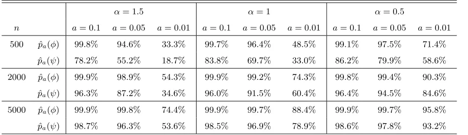
the roots are real). For each model, Table 1 reports the empirical frequencies of estimators that are sufficiently close to the actual values of the roots. As expected, the accuracy increases withn

but, more strikingly, it increases sharply asα approaches zero.

α= 1.5 α= 1 α= 0.5

n a= 0.1 a= 0.05 a= 0.01 a= 0.1 a= 0.05 a= 0.01 a= 0.1 a= 0.05 a= 0.01

500 pˆa(φ) 99.8% 94.6% 33.3% 99.7% 96.4% 48.5% 99.1% 97.5% 71.4%

ˆ

pa(ψ) 78.2% 55.2% 18.7% 83.8% 69.7% 33.0% 86.2% 79.9% 58.6%

2000 pˆa(φ) 99.9% 98.9% 54.3% 99.9% 99.2% 74.3% 99.8% 99.4% 90.3%

ˆ

pa(ψ) 96.3% 87.2% 34.6% 96.0% 91.5% 60.4% 96.4% 94.5% 84.6%

5000 pˆa(φ) 99.9% 99.8% 74.4% 99.9% 99.7% 88.4% 99.9% 99.7% 95.8%

ˆ

pa(ψ) 98.7% 96.3% 53.6% 98.5% 96.9% 78.9% 98.6% 97.8% 93.2%

Table 1: Accuracy of the roots-estimation through backward LS: ˆpa(θ) denotes the frequency of estimations ˆθ

belonging to the set

θˆ−θ0< a ∩ _ˆ

θ∈R _{, for θ =φ or ψ, fora = 0.01, 0.05, 0.1 and over 100,000 simulated}

paths of theα-stable MAR(1,1) process (Xt) solution of (1−ψ0F)(1−φ0B)Xt=εt, withψ0= 0.7 andφ0= 0.9.

Turning to the asymptotic distribution of (ˆη1,ηˆ2), results reported in the Supplementary file

strong representation. Given that the residuals autocorrelations of this pure causal AR have the same asymptotic distribution as those of the all-pass causal representation, the procedure remains valid.15 We therefore proceeded with this methodology (see the Supplementary file). The empirical sizes of the 1, 5 and 10% nominal tests for lags H = 1, . . . ,10 are reported in Table 2. It can be seen that using the Monte Carlo procedure, the portmanteau test is much better behaved in finite sample, especially for α= 1.5, which is a realistic value for financial series.

α= 1.5 α= 1 α= 0.5

H 1% 5% 10% 1% 5% 10% 1% 5% 10%

1 1.30 5.80 10.5 1.25 5.40 10.4 1.45 4.10 7.35

2 1.55 5.65 10.9 1.60 5.25 9.65 1.35 3.90 7.05

3 1.40 5.35 10.9 1.30 5.05 9.40 1.20 4.45 6.95

4 1.50 5.45 10.5 1.35 5.00 9.90 1.20 4.35 7.00

5 1.25 5.50 9.85 1.20 4.90 9.20 1.10 4.20 7.30

6 1.30 5.00 10.1 1.05 4.70 9.40 1.10 4.25 7.40

7 1.20 5.25 9.75 1.05 4.40 9.15 1.20 4.00 7.50

8 1.10 5.25 9.75 1.15 4.55 8.70 1.05 3.70 7.25

9 1.25 5.10 9.80 1.30 4.30 8.60 1.05 3.75 7.50

10 1.35 5.10 10.1 1.20 4.55 8.70 0.90 3.65 7.15

Table 2: Empirical sizes (%) of the portmanteau statistics (4.13) implemented by the Monte Carlo test procedure. The empirical size was calculated based on 2000 simulations of the α-stable MAR(1,1) process (Xt) solution of

(1−ψ0F)(1−φ0B)Xt = εt, with ψ0 = 0.7 and φ0 = 0.9. Each Monte Carlo test was performed with 1000

simulations.

5.2 Selection based on extreme residuals clustering

We now gauge the usefulness of the results of Section 4.5 by simulating paths of the α-stable MAR(1,1) process (1−ψ0F)(1−φ0B)Xt =εt with different parameterisations and analysing the

residuals of the competing representations. There are four competing models yielding the same

15

It can indeed be noticed that the asymptotic distributions of the LS estimator and of the residuals autocorrelations

all-pass causal AR(2) representation:

Pure causal AR(2): (1−ψ0B)(1−φ0B)Xt=ζt, (5.1)

MAR(1,1): (1−ψ0F)(1−φ0B)Xt=εt, (5.2)

MAR(1,1): (1−ψ0B)(1−φ0F)Xt=νt, (5.3)

Pure noncausal AR(2): (1−ψ0F)(1−φ0F)Xt=ωt, (5.4)

where (ζt), (νt) and (ωt) denote the sequences of errors of each all-pass representations. More

specifically for each estimated model, we compute the errors at several horizons h (as in (4.18)-(4.19) for the AR(1). For each MAR(1,1) alternatives, we disentangle the causal and noncausal components and compute their respective error series). For each errors series and a given threshold

x > 0, we identify the clusters of consecutive extreme values, i.e., errors larger than x in modu-lus. As explained in Section 4.5, for any horizon h, we expect all-pass representations to display larger clusters of extreme errors than the strong model, for which clusters larger thanh have zero probability. Letting ˆξk,h(x) denote the number of consecutive exceedances for the k-th cluster, we

therefore propose an Excess Clustering (EC)16 indicator defined as:

ECh=

P

k/ξˆk,h(x)>h

ˆ

ξk,h(x)−h

Card{k: ˆξk,h(x)> h}

, if Card{k: ˆξk,h(x)> h}>0, else ECh = 0. (5.5)

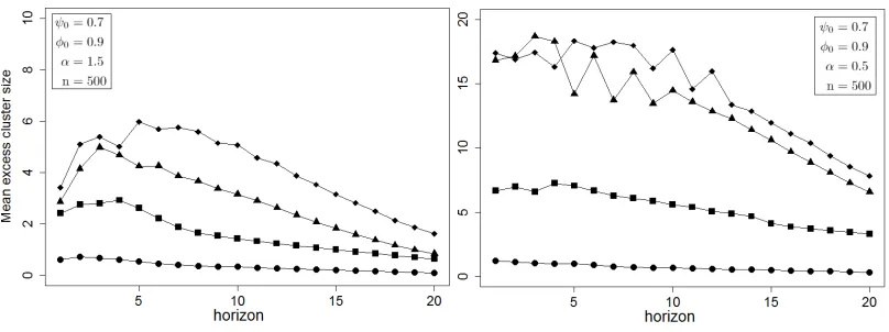
We start by generating 10000 sample paths of MAR(1,1) processes. For each path, we fit a backward AR(2), estimate the set{φ0, ψ0}, and for each of the four competing models we estimate

a term structure of residuals excess clustering with respect to the horizon, using the indicator (5.5). Averaging model-wise across the 10000 simulations yields the typical excess clustering behaviours of the residuals of each competing models. We perform this experiment for several MAR(1,1) processes and display the results of two parameterisations in Figure 3 (see the Supplementary file for additional results and details regarding the methodology).

It can be noticed that the all-pass models feature excessively clustering residuals at any horizon whereas the residuals of the strong model are barely deviating from no excess clustering. As we could expect from (4.16), the heavier the tails the easier it is to identify dependent residuals. This

16

For a given h, ECh defined at (5.5) corresponds to the average size of clusters larger than h, from which we

subtracth, and is 0 if all the clusters are smaller thanh. It is related to the Extremal Index, more common in the

literature, which is the reciprocal of the average size of clusters. Also, the choice of clustering scheme, i.e. how the

sequence ( ˆξk,h(x))kis constructed, can have an impact on the estimated excess clustering : more elaborate clustering

is in line with the findings of Hecq, Lieb and Telg (2016) who are concerned with identification of causal/noncausal models using the LAD estimator. Noticeably, even with very heavy tails (α = 0.5), the residuals at any horizons of the strong representation still barely deviate from no excess clustering. These experiments highlight in addition the usefulness of considering residuals at various horizons, instead of focusing only on basic residuals. Indeed, all the term structures of excess clustering show that the contrast between the competing models does not arise for h = 1 but rather tends to peak for intermediate values ofh.

Last, we assess how well we can discriminate between the all-pass models and the strong representation by exploiting the excess clustering feature. For each of the 10,000 simulations, we rank the four competing models according to the area under the term structure curve of excess clustering (AUC) and select the candidate with least AUC. Table 3 reports the true positive rates of this procedure. For α = 1.5 andn = 500, the strong representation was correctly identified in above 88% of the 10,000 simulated paths and this proportion increases withn.

n= 500 n= 2000 n= 5000 88.4% 95.8% 97.5%

Table 3: Correct model selection rates based on least excess clustering across 10,000 simulated paths of the MAR(1,1) process (Xt) solution of (1−0.7F)(1−0.9B)Xt=εt with i.i.d. 1.5-stable noise.

Figure 3: Across 10,000 simulations of theα-stable MAR(1,1) process (Xt) solution of (1−ψ0F)(1−φ0B)Xt=εt,

average of the term structure of excess clustering of the linear residuals of the four competing models (5.1) (squares),

the strong representation (5.2) (points), (5.3) (triangles) and (5.4) (diamonds). The parameterisations and path

6

An application to financial series

In this section, we illustrate the adequacy of MAR models for real economic series. We fitted MAR models on six financial series of monthly prices: stock prices of Coca-Cola (January 1978 to June 2017), Boeing (February 1962 to December 2012), Hong Kong’ stock market index (HSI) (December 1986 to April 2017), Walmart (September 1979 to June 2017), Exxon (February 1970 to June 2017), and the quarterly Shiller Price/Earning ratio (1881 to 2017). All the series, pictured on Figure 4, have been centered and a linear deterministic trend has been fitted and subtracted.

6.1 AR estimation and validation using the Monte Carlo Portmanteau test

We start by investigating the appropriate total AR order (r =p+q) for each series using the Monte Carlo portmanteau test of Section 5.1. For each series, starting from total AR order 1, we estimate all-pass causal representations of increasing order by LS and perform the portmanteau test with

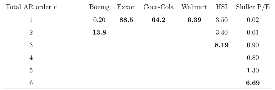
H = 50 lags using the Monte Carlo portmanteau procedure of Lin and McLeod (1000 paths were simulated for each test). The results of the portmanteau test, reported in Table 4, allow to discard non-admissible low order models at the level 5%. We retain for the following the lowest orders (indicated in bold) which pass the portmanteau procedure: Boeing: 2; Exxon: 1; Coca-Cola: 1; Walmart: 1; HSI: 3; Shiller P/E: 6.17

Total AR order r Boeing Exxon Coca-Cola Walmart HSI Shiller P/E

1 0.20 88.5 64.2 6.39 3.50 0.02

2 13.8 3.40 0.01

3 8.19 0.90

4 0.80

5 1.30

6 6.69

Table 4: P-values (%) of the Monte Carlo portmanteau tests withH = 50 lags for increasing AR orderr. Rejection if P-value < 5%.

17

This procedure yields as a by-product the McCulloch quantile estimates of the tail index α (see McCulloch

(1986)) for the six financial series. Values of ˆα: Boeing: 1.79; Exxon: 1.69; Coca: 1.64; Walmart: 1.67; HSI: 1.38;

Figure 4: Financial series paths: Boeing (2/1962 to 12/2012), Exxon (2/1970 to 06/2017), Coca-Cola (1/1978 to 06/2017), Walmart (9/1979 to 6/2016), Hang Seng Index (HSI, 12/1986 to 05/2017) and the Shiller P/E ratio

(Q1/1881 to Q2/2017). All series are monthly except the latter which is quarterly. Each are centered and a linear

trend has been fitted and subtracted.

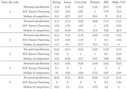
6.2 MAR selection based on extreme clustering

AR orderrthe MAR(p, q) specification which displays the lowest AUC of excess clustering and the median AUC of its competitors. The favoured specification of some series feature very low AUC excess clustering even for total AR orderr = 1 (e.g. Walmart, Coca-Cola), whereas others display high excess clustering for low total AR order (e.g. Boeing, Shiller P/E). We can notice that for the latter, excess clustering rapidly decreases as r increases. Besides, we can also see a general decreasing trend for median excess clustering of competing models asr increases.

Combining the results from the portmanteau tests of the previous Section and of the extreme clustering analysis, we select a final specification for each series as follows. For a given series,

• Assign the total AR orderr validated by the portmanteau test (see Table 4).

• For the assigned orderr, select then the least excess clustering competing representation (see the favoured specifications in Table 5).

The selection is reported in Table 6 which shows the causal and noncausal orders as well as the (in-verted) roots of the corresponding polynomials. On the one hand, three series have been identified as pure noncausal AR(1): Exxon, Coca-Cola, Walmart, which is compatible we the fact that they all display multiple bubble patterns followed by sharp drops. On the other hand, the remaining series display more complex dynamics (Boeing, HSI, Shiller P/E ratio). Noticeably, the presence of bubbles in the HSI is unclear. Clear-cut drops are not visible which is compatible with the high causal root identified.

7

Concluding remarks

Total AR order Boeing Exxon Coca-Cola Walmart HSI Shiller P/E

Favoured specification (1,0) (1,0) (1,0) (1,0) (0,1) (1,0)

1 AUC Excess Clustering 8.67 3.25 2.67 1 7.75 15.6

Median of competitors 31.1 25.7 51.7 29.3 17 51.2

Favoured specification (1,1) (1,1) (2,0) (2,0) (1,1) (1,1)

2 AUC Excess Clustering 5.33 2.75 1.67 1 5.75 9.58

Median of competitors 14.2 13.58 27.8 15.0 9.33 25.5

Favoured specification (2,1) (1,2) (1,2) (3,0) (1,2) (1,2)

3 AUC Excess Clustering 5.15 2.25 1.33 1 0.5 1.64

Median of competitors 11.5 13.1 27.7 10.5 6.17 8

Favoured specification (2,2) (3,1) (4,0) (4,0) (1,3) (1,3)

4 AUC Excess Clustering 7.05 3 1 1 0.5 2.13

Median of competitors 15.2 6.63 11.7 9.57 5.66 5.95

Favoured specification (4,1) (5,0) (5,0) (5,0) (3,2) (3,2)

5 AUC Excess Clustering 3.5 0 1 1 2 2

Median of competitors 12 8.64 12.9 6.74 5.67 4.88

Favoured specification (6,0) (5,1) (6,0) (6,0) (1,5) (2,4)

6 AUC Excess Clustering 3 0 0 0 0.5 1.33

Median of competitors 10.3 5.5 11.4 5.73 4.2 5

Table 5: Selection based on extreme clustering.

Series Final specification Noncausal (inverted) roots Causal (inverted) roots

Boeing MAR(1,1) 0.95 0.18

Exxon MAR(1,0) 0.95 −

Coca-Cola MAR(1,0) 0.90 −

Walmart MAR(1,0) 0.91 −

HSI MAR(1,2) 0.37 −0.27, 0.89

Shiller P/E MAR(2,4) 0.58±0.29i −0.21±0.6i, 0.96,−0.70

Table 6: Selection of the MAR specification for each financial series among the favoured ones of Table 5 based on the total AR order determined in Table 4. The MAR(p, q) specifications indicate the noncausalpand causalqorders

as well as the (inverted) roots of the corresponding polynomials.

noncausal processes. We proposed an alternative strategy based on extreme clustering and leave its asymptotic properties for further investigations.

Appendix: Proofs

A

Proof of Proposition 2.1

Using the MA(∞) representation (2.3) ofXtand the assumption thatεti.i.d.∼ S(α, β, σ, µ), it follows

that

∀s∈R_{, ψX}

t(s) :=E h

eisXti_=E   e is +∞ P

k=−∞

dkεt+k 

 =

+∞

Y

k=−∞

Eh_eisdkεt+ki

=

+∞

Y

k=−∞

exp{−σα|dks|α(1−iβsign(dks)w(α, dks)) +idksµ}.

Ifα6= 1, then,

∀s∈R_{, lnψXt(s) =}

+∞

X

k=−∞

−σα|dks|α

1−iβsign(dks)tg

_πα

2

+idksµ

=−σ˜α|s|α



   

1−iβ

+�