Testing an Information Intervention: Experimental Evidence on the Effect of Jamie Oliver on Fizzy Drinks Demand

(1)

Munich Personal RePEc Archive

Testing an Information Intervention:

Experimental Evidence on the Effect of

Jamie Oliver on Fizzy Drinks Demand

Gibson, John and Tucker, Steven and Boe-Gibson, Geua

University of Waikato

29 May 2019

Online at

https://mpra.ub.uni-muenchen.de/94182/

(2)

June, 2019

Testing an Information Intervention:

Experimental Evidence on the Effect of Jamie Oliver on Fizzy Drinks Demand

John Gibson, Steven Tucker, and Geua Boe-Gibson

Department of Economics, University of Waikato, Hamilton, New Zealand

Abstract

We conducted a salient purchasing experiment to test if an information intervention alters fizzy drinks demand. Subjects in our experiment initially made five rounds of purchases, for 14 items (energy drinks, colas, and lemonades) selected from a stratified sample of retailers. Subjects faced seven pricing environments, reflecting baseline prices, two ad valorem taxes, two specific taxes, and ad valorem and specific price cuts to reflect retailer discounting. Subjects then watched a video presentation by celebrity chef Jamie Oliver, which highlighted adverse health effects of sugary drinks. The five rounds of choices were then repeated, to generate within-subject before and after demands that show an overall 25% reduction in purchases due to the information intervention. Demand for one sugar-free option, Diet Coke, rose 36% after the intervention. The impacts under baseline prices were little different to those seen in conjunction with tax-induced price rises. Effects of the information intervention were larger for females, for the young, for the less educated, for those usually spending more on soft drinks, and for those who usually ignore sugar content when making purchases.

JEL Codes: C91, D83, I18

Keywords: Experiment, Health, Information, Jamie Oliver, Soda taxes, Sugar

Acknowledgements: We thank Andrew Gera and Myles McInnes for assistance. Funding support from

(3)

1

I. Introduction

The focus of policymakers and researchers concerned about health effects of sugar-sweetened beverage (SSB) consumption is mainly on fiscal measures, like soda taxes, rather than on information interventions. Over 20 countries now have some form of soda tax, including France, Mexico, Norway, and the U.K. (Baker et al, 2017). The World Health Organization suggest taxes to raise retail price of SSBs at least 20% will reduce consumption proportionately (WHO, 2016). Less attention is paid to information interventions, such as health warnings, despite the evidence from tobacco control that such warnings promote smoking cessation and discourage youth uptake (see Hammond, 2011, for a review of this evidence).

Information interventions may be as effective as taxes in moderating SSB consumption, for two reasons. First, predicted effects of soda taxes often rely on studies that ignore responses that mediate how price rises translate into changes in quantity consumed. The first response is stocking. If consumers buy when prices are temporarily lower and stockpile to consume later, the own-price elasticity of quantity demand for soda is exaggerated up to 60% if this response is ignored (Wang, 2015). The second response is within-group quality substitution, if higher prices cause consumers to switch to cheaper variants, like discount brands and larger containers. Gibson and Romeo (2017) and Gibson and Tucker (2018) show that if lower spending due to adjusting quality is misinterpreted as a quantity response, own-price elasticities of quantity demand for SSBs are overstated by as much as two- to three-fold. Andalón and Gibson (2018) find a similar overstatement, which flows through to overstated predictions of body mass reductions and health effects from Mexico’s peso-per-liter soda tax.

(4)

2

An issue with observational settings is that anticipatory responses, like stocking, and spillovers, if information spreads, may also affect demand. A laboratory experiment gives clean evidence on effects of an intervention because all other factors can be held constant. Therefore, we carried out an experiment to see how an information intervention affects SSB demand. Subjects in our experiment initially made five rounds of purchases, for 14 beverages (energy drinks, colas, and lemonades) in seven pricing environments. Subjects then watched a video presentation by celebrity chef Jamie Oliver highlighting adverse health effects of SSBs. The five rounds of choices were then repeated, to generate within-subject before and after demands. The quantity purchased fell by up to 50% for some SSBs after exposure to the information. Demand for one sugar-free option, Diet Coke, rose 36% after the intervention. Impacts under baseline prices were little different to those seen in conjunction with tax-induced price rises.

Our use of the term “experiment” follows standard use in economics, because we rely on directly observable salient behavioral responses, rather than on answers to hypothetical questions. Subjects faced real consequences of their choices, with one of the ten rounds and one of the seven price structures randomly chosen to pay out on the experimental demands. Many subjects left our laboratory carrying drinks that resulted from their actual purchase decisions. In contrast, most prior studies use hypothetical situations, even if authors title their studies ‘experimental’ (e.g. Bollard et al, 2016). These studies typically use online surveys to see if graphic warnings (e.g. with pictures of dental caries) or plain packaging affect self-reported SSB purchase intentions (Billich et al, 2018). However, because “talk is cheap” if there are no real behavioral consequences (Galizzi and Wiesen, 2017), the fact that these studies find that warning labels can cut hypothetical SSB demand by almost 60% is no real help for policymakers.

The next section briefly reviews related research using experiments. We describe our experiment and the information intervention in Section 3. In Section 4 we report the results, relying especially on within-subject before and after comparisons to get at causal effects of the intervention. Section 5 has the conclusions.

II. A Brief Review of Related Experiments

A growing literature uses experiments to estimate effects of price manipulation and information interventions on food and beverage consumption decisions.1_{Some studies use laboratory, field}

or virtual experiments to collect consumption decisions in environments of supermarkets

(5)

3

(Epstein et al, 2015; Velema et al, 2017), or cafeterias and restaurants (Horgen and Brownell, 2002; Michels et al, 2008; Giesen et al., 2011; Streletskaya et al, 2014). Some studies have potentially problematic design issues because they either involve only hypothetical scenarios, have few or very small price changes, or have no budget constraints to restrain purchases.

Yang and Chiou (2010) account for some of these issues in their laboratory experiment, in a 22 design with health information and drink price as treatment variables. Subjects in the information treatment were primed with an article discussing obesity issues relating to sugary beverages and the importance of healthy diet. Participants sampled a selection of four healthy and unhealthy beverages, ranked their preferences, and then could purchase their most favored healthy and unhealthy beverage at five different price levels, using a $7 endowment. Choices at one price level were selected randomly to be realized. Yang and Chiou find that providing health information promotes substitution away from unhealthy beverages.

Streletskaya et al (2014) also use a 22 design, simulating a cafeteria environment with a single price change (an unhealthy food tax and healthy food subsidy) and information in the form of anti-obesity and healthy food advertising. Participants were given a $10 voucher to spend on a lunch menu that had both healthy and unhealthy options. Prior to their consumption decisions, participants viewed a television show with advertisements specific to their treatment. Subjects made consumption decisions across six treatments, with one selected randomly to be realized. A combined unhealthy food tax and anti-obesity advertisements promoted healthier choices, while a subsidy and advertisements favoring healthy foods had little effect. There was no effect of anti-obesity advertisements by themselves.

While designs of the two papers discussed above address some issues that plague other experiments in this area, there are still potential problems.2_{Neither study let subjects keep}

unspent portions of their endowment, and so there are no opportunity costs of decisions. There was also no procedure to ensure that products were representative of daily consumption options available to subjects, and baseline prices were not chosen to match purchasing options outside the laboratory. Finally, there was no baseline treatment without priming. Our experimental design addresses all of these potential problems.

III. Methods

3.1 Overview

Our experimental design builds upon Gibson and Tucker (2018) that examined quality and

(6)

4

quantity responses to pricechanges for fizzy soft drinks. A feature of the current experiment is the provision of health-related information, which was not previously considered.

3.2 Products

To ensure we used representative items, we surveyed a nearby supermarket (a 20 minute walk from the laboratory), local convenience stores, and all outlets on campus. The supermarket had 160 specifications of fizzy drinks and the convenience stores had 104 specifications. Prices averaged NZ$5.30 per liter (SD=$2.80 per liter).3_{The range on campus was more limited, with}

just 12 specifications, priced higher (average $8.60 per liter). We selected 21 items with probability proportional to size (the count of items on shelf display) from the combined supermarket and convenience store frames. After pre-testing, we dropped items larger than one liter, which were awkward for student subjects to carry to classes after the lab sessions.4

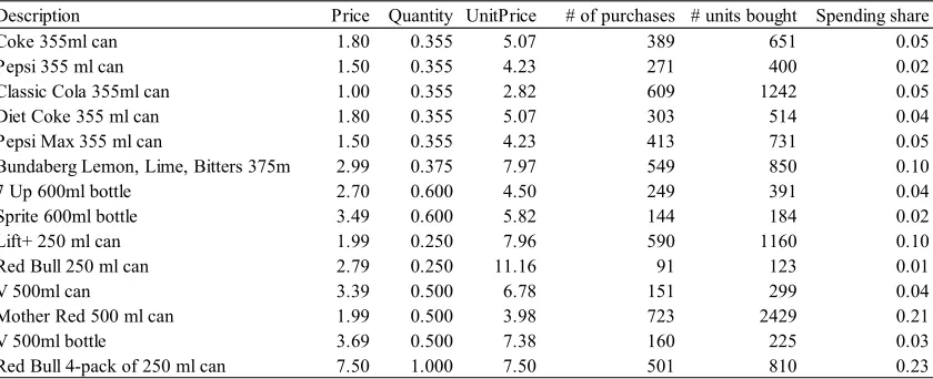
Table 1 describes the 14 items we use, which include six energy drinks, five colas, and three other soft drinks (a ‘lemonades’ group). The mean unit price is $6.00 per liter (SD=$2.20). We lack bulky (hence, cheaper) items but otherwise our products are representative. The last three columns of Table 1 show purchase occasions in the experiment, the number of units bought, and the share of spending for each item. Our experiment generated n=5,143 purchases with just over 10,000 units bought, with multiple-unit purchases especially for single cans of energy drinks (Mother, V, Lift+) and a discount cola (Classic Cola). Overall, 63% of total spending was on energy drinks, 21% on colas, and the remainder on lemonades.

(Table 1 about here) 3.3 Subjects

The 110 subjects were recruited university-wide. The median age was 24 years, 45% were male, 80% were undergraduates, and median education was 15 years. Their mean weekly spending was $8 on fizzy drinks (median $5), out of $250 per week total spending.

3.4 Experiment

The experiment took place in the Waikato Experimental Economics Laboratory (WEEL), that allows private decision-making. We ran sessions over five months from late 2017. The sessions typically lasted just over one hour to go over instructions, complete a background survey, make the initial choices over five rounds of the experiment, watch the video, have another five rounds of choices, and finally receive in-kind and in-cash payments.

3_{At the time of the experiment, the exchange rate averaged NZD$1=USD$0.71.}

4_{The decreases in quantity purchased due to the information intervention that we report below may be lower}

(7)

5

Subjects were given an endowment of cash each round, which stochastically varied from $18 to $24 with mean $21. The individual endowment was private information and the distribution of endowments was not revealed to subjects. The prices also (slightly) varied stochastically by round, to reflect the distribution of prices observed across outlets.

Within each round, subjects made purchase decisions under seven pricing schemes: one reflects the baseline prices, two reflect price rises from ad valorem taxes of 20% and 40%, two reflect price rises from excise taxes of 50 cents and $1 per liter, and two are price cuts of 20% and 50 cents per liter, which were included in case responses are not symmetric when prices rise and fall. To guard against framing effects, we did not refer at any point to taxes; the pricing schemes were simply numbered as #1 to #7. To guard against ordering effects, subjects saw all seven pricing schemes on a single decision screen that displayed the matrix of prices for all schemes and for all drinks in that round.

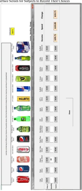
Subjects could work in any order they liked, but for each scheme they had to open a pop-up interface, shown in Figure 1. Within this pop-up, they could spend as much (up to the value of their daily endowment) or as little on drinks as they liked. The pop-up listed the prices for each drink under the current pricing scheme and had input boxes to enter the number of units they wanted to purchase (e.g. 10 cans of Classic Cola in Figure 1). These input boxes were aligned with pictures of each product, and the 14 drinks were available for viewing at the front of the laboratory, presented in the same order as on the screen.

(Figure 1 about here) 3.5 Incentives

After all subjects made their purchase choices, one round and one pricing scheme were selected using a bingo cage. Transactions from that round became the realized decisions. Subjects were then called back to the payment room, one at a time, to privately receive their purchased drinks and any residual cash. The combined in-kind and in-cash remuneration was worth $22, on average. This is just under 10% of median weekly spending on food, drink, and rent.

3.6 Information Intervention

After the 5th_{round, subjects privately watched a ten minute excerpt from}_{Jamie’s Sugar Rush}_,

(8)

6

provided was focused on health consequences of SSB consumption. After watching the video, subjects answered qualitative questions related to awareness of material in the documentary and then had a further five rounds of purchases, where the endowments and prices they had faced in rounds 1-5 were repeated. Thus, we have within-subject before and after comparisons, where the only factor that changed is awareness of some health consequences of consuming fizzy drinks.

IV. Results

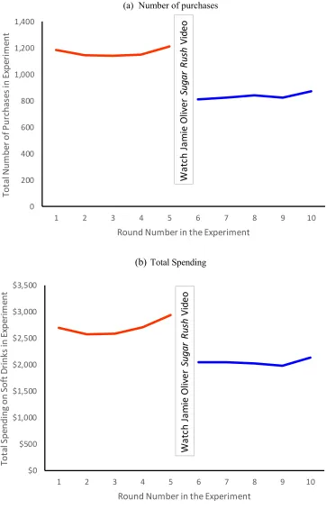
After watching the Sugar Rush video, demand declined sharply. The evolution of the total number of purchases (in panel a) and the total spending on drinks (in panel b) across ten rounds of the experiment is shown in Figure 2. There is no trend in either series, from Round 1 to Round 5, or again from Round 6 to Round 10. However, there is a sharp discontinuity, with a 28% drop in the number of purchases and a 24% drop in the total spending, between the first five and second five rounds. The only difference between these two sets of five rounds was the introduction of the new information, in the Sugar Rush video.

(Figure 2 about here)

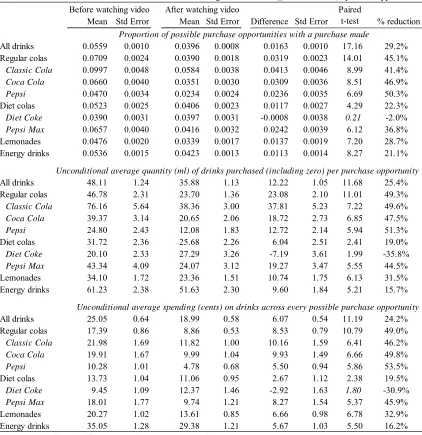
In Table 2 we exploit the paired nature of the within-subject change our experiment allows. We consider three decisions subjects faced: whether to take up a purchase opportunity; what quantity to purchase; and, the total spending on drinks. We present results by type of drink, and also by individual item for colas, which received a lot of attention in the Jamie Oliver video (e.g., with footage of babies in Mexico drinking Coca Cola). Our interest is in the unconditional averages, before and after watching the Sugar Rush video. These capture demand changes on both the extensive and intensive margins and are the statistic of interest for policy makers concerned with reducing population intake of sugar. The statistical significance of the difference between the pre-video and post-video averages is then examined with a paired t-test.

(Table 2 about here)

Across all purchase opportunities (for 14 drinks and seven pricing structures), subjects made a purchase on 5.6% of occasions (SE=1.0%) in the first five rounds. This rate fell to 4.0% after watching the video and the difference of 1.6 percentage points is precisely estimated (SE=0.1 percentage points). In proportionate terms, watching the video caused a 29% decrease in the odds of purchasing fizzy drinks. The unconditional average quantity purchased was 48ml before the video and 36ml after the video (a 25% reduction), while unconditional average spending fell from 25 cents to 19 cents (a 24% reduction).

(9)

7

by 3.2 percentage points, or 45% of the pre-video level. The demand for two sugar-free colas showed contrasting patterns; the probability of purchasing Diet Coke rose, while it fell by 2.4 percentage points (37% of the pre-video level) for Pepsi Max. Notably, the “no sugar” statement on the Pepsi Max can is much more discretely placed (with a far smaller font) than the word “Diet” on a Diet Coke can, so subjects may have thought of Pepsi Max as regular cola (given that we were replicating information environments in typical shopping scenarios, we provided no additional information pertaining to which drinks were sugar-free and which were not). Apart from Diet Coke, the energy drinks had the smallest reductions in demand after subjects had watched the video, with the odds of a purchase falling 21%.

The remaining two panels of Table 2 show the effect of the intervention on the quantity of soft drinks purchased, and on total spending on these drinks. There was a shift in demand towards Diet Coke, whose average quantity purchased rose by 7ml while demand for the other colas was 42ml lower; in proportionate terms this represented a 36% rise in demand for Diet Coke while demand for the other colas fell by 47%. The energy drinks were the category whose demand was least affected by the information intervention; quantity purchased and spending fell by just 16%. Notably, energy drinks were not highlighted in the Sugar Rush video.

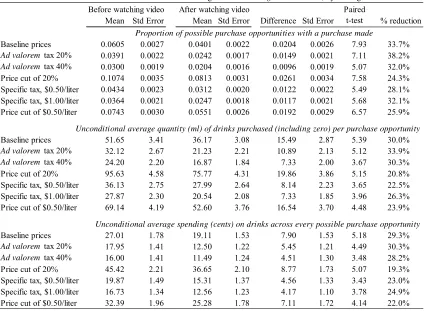
The results reported in Table 3 consider how the demand reductions after watching the video varied with the different pricing structures. At baseline prices, which reflected prices in local off-campus outlets, there was a 34% fall in the probability of a purchase, a 30% fall in the quantity purchased and a 29% fall in spending. The proportionate reductions in purchase odds were slightly larger when prices reflected a 20% ad valorem tax but in an environment with even higher prices, from a 40% ad valorem tax, demand falls after watching the video were slightly less than at baseline prices. If the pricing environment had specific taxes, the impact of the video on demand was a little less than with either ad valorem taxes or at baseline prices, especially for the quantity purchased.5_{However, the variation due to either type of tax}

compared to the effect seen with baseline prices is fairly small. A reasonable summation is that effects of the information intervention at baseline prices are little different to those seen in conjunction with tax-induced price rises.

Two other notable features in Table 3 are the asymmetric responses to price cuts versus

5_{In addition to looking along rows of Table 3, to see impacts of the information intervention, looking down the}

(10)

8

rises, and a tax-induced price structure with similarly suppressed demand as for the information intervention. At baseline prices, watching the video caused purchase probabilities to drop two percentage points, and mean quantity purchased fell by 15ml. These effects are most similar to the pre-video results where prices reflect a specific tax of $0.50 per liter, which could be considered the tax-equivalent value of the information intervention. With price cuts of either 20% ad valorem or $0.50 per liter, demand rose, in terms of purchase probabilities and quantities, by more than twice as much as the fall in demand with taxes of either 20% or $0.50 per liter. One consequence of the large demand response to price cuts is that the proportionate reduction in demand due to watching the video is smaller than under other pricing structures because of the higher level of pre-video demand.6

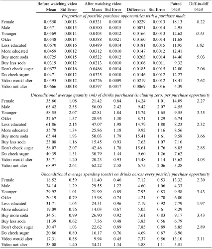
There was considerable heterogeneity in the effects of the information intervention, which is highlighted in Table 4. In terms of demographic characteristics, the effects of the information intervention were larger for females, for the young, and for the less educated. In each case, we use a difference-in-differences strategy by contrasting the within-subject before and after comparison of demands for two mutually exclusive groups. For example, the odds of a female subject purchasing a soft drink fell by 2.3 percentage points after the video, while for males the fall was only by 0.7 percentage points (with a t-statistic of 8.22 for the difference in the differences). Likewise, subjects who were below the median age reduced their quantity purchased by 16ml after the video, while older subjects cut average demand by only 9ml, and the gap for the less educated versus the more educated was almost as large.

In addition to demographics, we also considered three behavioral-related variables that may be relevant to the effect of the information intervention: whether the typical amount spent on soft drinks was above the median of $5 per week (“buy more soda”); whether the subject typically considered sugar content when making purchases (“check sugar”); and, whether the subject rated the Jamie’s Sugar Rush video as likely to change their future consumption decisions (“video would alter”) where this rating was made immediately after seeing the video but before having the chance to make purchases in Rounds 6 to 10. There was a larger effect of the information intervention on subjects who typically buy more soda, reducing their odds of buying and their average quantity by twice as much as for the “buy less soda” group. There

6_{The asymmetry is not because taxes do not apply to the two sugar-free drinks, to consider effects of a SSB tax}

(11)

9

were also significantly larger effects of the intervention on subjects who usually ignore sugar content when making purchases, with t-statistics for the difference-in-differences which ranged from 2.1 to 2.9 for the three types of decisions shown in Table 4. The subjects who said that the information in the video would affect their future consumption did indeed show this, with their reduction in spending, in quantity bought, and in odds of purchasing being from two to three times larger than for the subjects who felt that the information would not change their future consumption decisions (“video not alter”).

V. Conclusions

Compared to attention paid to fiscal measures, like soda taxes, there is far less evidence on how information interventions alter demand for sugar-sweetened beverages. This is despite the key role of health warnings in reducing smoking. Apart from the intriguing result of Taylor et al (2019), that information from the Berkeley soda tax debate, rather than price changes per se, seemed to reduce demand for regular soda demand and raise demand for diet soda, there is little research by economists on effects of information on soda demand. While there is public health research on this topic, it is mostly for hypothetical demands, and typically uses online surveys, and thus does not provide a firm foundation for guiding policymakers.

To contribute to this gap in the literature, we designed an incentivized laboratory experiment, where the within-subject before and after design lets us see how exposure to health information affects demand for fizzy soft drinks. The health information was given in a style likely to be salient for young people, drawing on a documentary presented by the celebrity chef Jamie Oliver. We find that quantity purchased fell by up to 50% for some SSBs after exposure to this information, while demand for one sugar-free option, Diet Coke, rose 36%. The fall in demand due to the information intervention is about the same as the response to a $0.50 per liter excise tax. The impacts of the information intervention were largely unchanged if prices were raised moderately by taxes, but became smaller at higher prices.

(12)

10

References

Andalón, M., Gibson, J. 2018. The ‘soda tax’ is unlikely to make Mexicans lighter or healthier: New evidence on biases in elasticities of demand for soda. MPRA Paper No. 86370. Baker, P., Jones, A., Thow, A. 2017. Accelerating the worldwide adoption of sugar-sweetened

beverage taxes: Strengthening commitment and capacity. International Journal of Health Policy and Management 6(1): 1-5.

Billich, N., Blake, M., Backholer, K., Cobcroft, M., Li, V., Peeters, A. 2018. The effect of sugar-sweetened beverage front-of-pack labels on drink selection, health knowledge and awareness: An online randomised controlled trial. Appetite 128(1): 233-241. Bleich, S., Barry, C., Gary-Webb, T., Herring, B. 2014. Reducing sugar-sweetened beverage

consumption by providing caloric information. American Journal of Public Health 104(12): 2417-2424.

Bollard T, Maubach N, Walker N, Mhurchu C. 2016. Effects of plain packaging, warning labels, and taxes on young people’s predicted sugar-sweetened beverage preferences: an experimental study. International Journal of Behavioral Nutrition and Physical Activity 13(1): 1-7.

Epstein, L., Finkelstein, E., Katz, D., Jankowiak, N., Pudlewski, C., Paluch, R. 2016. Effects of nutrient profiling and price changes based on NuVal® scores on food purchasing in an online experimental supermarket. Public Health Nutrition 19(12): 2157-2164. Epstein, L., Jankowiak, N., Nederkoorn, C., Raynor, H., French, S., Finkelstein, E. 2012.

Experimental research on the relation between food price changes and food-purchasing patterns: A targeted review. The American Journal of Clinical Nutrition 95(4): 789-809.

Fischer, A., 2014. Some comments on “Taxes, Subsidies, and Advertising Efficacy in Changing Eating Behavior: An Experimental Study”. Applied Economic Perspectives and Policy 36(4): 717-721.

Galizzi, M., Wiesen, D. 2017. Behavioral experiments in health: An introduction. Health Economics 26(S3): 3-5.

Gibson, J., Romeo, A. 2017. Fiscal‐food policies are likely misinformed by biased price

elasticities from household surveys: Evidence from Melanesia. Asia & the Pacific Policy Studies 4(3): 405-416.

(13)

11

Giesen, J., Payne, C., Havermans, R., Jansen, A. 2011. Exploring how calorie information and taxes on high-calorie foods influence lunch decisions. The American Journal of Clinical Nutrition 93(4): 689–694

Hammond, D. 2011. Health warning messages on tobacco products: a review. Tobacco Control 20(5): 327-337.

Horgen, K., Brownell, K. 2002. Comparison of price change and health message interventions in promoting healthy food choices. Health Psychology 21(5): 505-512.

Michels, K., Bloom, B., Riccardi, P., Rosner, B., Willett, W. 2008. A study of the importance of education and cost incentives on individual food choices at the Harvard School of Public Health cafeteria. Journal of the American College of Nutrition 27(1): 6-11. Sharma, A., Hauck, K., Hollingsworth, B., Siciliani, L. 2014. The effects of taxing sugar‐

sweetened beverages across different income groups. Health Economics 23(9): 1159-1184.

Streletskaya, N., Rusmevichientong, P., Amatyakul, W., Kaiser, H. 2014. Taxes, subsidies, and advertising efficacy in changing eating behavior: An experimental study. Applied Economic Perspectives and Policy 36(1): 146–174.

Taylor, R., Kaplan, S., Villas-Boas, S., Jung, K. 2019. Soda wars: The effect of a soda tax election on university beverage sales. Economic Inquiry doi: 10.1111/ecin.12776 Velema, E., Vyth, E., Steenhuis, I. 2017. Using nudging and social marketing techniques to

create healthy worksite cafeterias in the Netherlands: intervention development and study design. BMC Public Health 17(1):63.

Wang, E. 2015.The impact of soda taxes on consumer welfare: implications of storability and taste heterogeneity. RAND Journal of Economics 46(2): 409-441.

Wilson, A., Buckley, E., Buckley, J., Bogomolova, S. 2016. Nudging healthier food and beverage choices through salience and priming. Evidence from a systematic review. Food Quality and Preference 51(1): 47-64.

World Health Organization [WHO]. 2016. Fiscal Policies for Diet and Prevention of Non-Communicable Diseases Technical Meeting Report, 5-6 May, Geneva, Switzerland.

http://apps.who.int/iris/bitstream/10665/250131/1/9789241511247-eng.pdf

(14)

[image:14.612.169.436.68.688.2]

12

(15)

[image:15.612.125.487.83.648.2]

13

Figure 2: Total Number of Purchases and Total Spending, by Round (a) Number of purchases

(b) Total Spending

0 200 400 600 800 1,000 1,200 1,400

1 2 3 4 5 6 7 8 9 10

To ta l N um be r o f P urc ha se s in Ex pe rim en t Round Number in the Experiment W at ch Ja m ie O live r Sugar Rus h Vi de o $0 $500 $1,000 $1,500 $2,000 $2,500 $3,000 $3,500

1 2 3 4 5 6 7 8 9 10

(16)

14

Description Price Quantity UnitPrice # of purchases # units bought Spending share

Coke 355ml can 1.80 0.355 5.07 389 651 0.05

Pepsi 355 ml can 1.50 0.355 4.23 271 400 0.02

Classic Cola 355ml can 1.00 0.355 2.82 609 1242 0.05

Diet Coke 355 ml can 1.80 0.355 5.07 303 514 0.04

Pepsi Max 355 ml can 1.50 0.355 4.23 413 731 0.05

Bundaberg Lemon, Lime, Bitters 375m 2.99 0.375 7.97 549 850 0.10

7 Up 600ml bottle 2.70 0.600 4.50 249 391 0.04

Sprite 600ml bottle 3.49 0.600 5.82 144 184 0.02

Lift+ 250 ml can 1.99 0.250 7.96 590 1160 0.10

Red Bull 250 ml can 2.79 0.250 11.16 91 123 0.01

V 500ml can 3.39 0.500 6.78 151 299 0.04

Mother Red 500 ml can 1.99 0.500 3.98 723 2429 0.21

V 500ml bottle 3.69 0.500 7.38 160 225 0.03

[image:16.612.98.518.76.247.2]

Red Bull 4-pack of 250 ml can 7.50 1.000 7.50 501 810 0.23

Table 1: Details on the Drinks in the Experiment

(17)

15

Mean Std Error Mean Std Error Difference Std Error % reduction

All drinks 0.0559 0.0010 0.0396 0.0008 0.0163 0.0010 17.16 29.2% Regular colas 0.0709 0.0024 0.0390 0.0018 0.0319 0.0023 14.01 45.1%

Classic Cola 0.0997 0.0048 0.0584 0.0038 0.0413 0.0046 8.99 41.4%

Coca Cola 0.0660 0.0040 0.0351 0.0030 0.0309 0.0036 8.51 46.9%

Pepsi 0.0470 0.0034 0.0234 0.0024 0.0236 0.0035 6.69 50.3%

Diet colas 0.0523 0.0025 0.0406 0.0023 0.0117 0.0027 4.29 22.3%

Diet Coke 0.0390 0.0031 0.0397 0.0031 -0.0008 0.0038 0.21 -2.0%

Pepsi Max 0.0657 0.0040 0.0416 0.0032 0.0242 0.0039 6.12 36.8%

Lemonades 0.0476 0.0020 0.0339 0.0017 0.0137 0.0019 7.20 28.7% Energy drinks 0.0536 0.0015 0.0423 0.0013 0.0113 0.0014 8.27 21.1%

Classic Cola 76.16 5.64 38.36 3.00 37.81 5.23 7.22 49.6%

Coca Cola 39.37 3.14 20.65 2.06 18.72 2.73 6.85 47.5%

Pepsi 24.80 2.43 12.08 1.83 12.72 2.14 5.94 51.3%

Diet colas 31.72 2.36 25.68 2.26 6.04 2.51 2.41 19.0%

Diet Coke 20.10 2.33 27.29 3.26 -7.19 3.61 1.99 -35.8%

Pepsi Max 43.34 4.09 24.07 3.12 19.27 3.47 5.55 44.5%

Lemonades 34.10 1.72 23.36 1.51 10.74 1.75 6.13 31.5% Energy drinks 61.23 2.38 51.63 2.30 9.60 1.84 5.21 15.7%

Classic Cola 21.98 1.69 11.82 1.00 10.16 1.59 6.41 46.2%

Coca Cola 19.91 1.67 9.99 1.04 9.93 1.49 6.66 49.8%

Pepsi 10.28 1.01 4.78 0.68 5.50 0.94 5.86 53.5%

Diet colas 13.73 1.04 11.06 0.95 2.67 1.12 2.38 19.5%

Diet Coke 9.45 1.09 12.37 1.46 -2.92 1.63 1.80 -30.9%

Pepsi Max 18.01 1.77 9.74 1.21 8.27 1.54 5.37 45.9%

[image:17.612.96.518.75.510.2]

Lemonades 20.27 1.02 13.61 0.85 6.66 0.98 6.78 32.9% Energy drinks 35.05 1.28 29.38 1.21 5.67 1.03 5.50 16.2% Note: Statistically insignificant t-test values (at p<0.05) are in italics

Table 2: Effects on Soft Drink Purchases of Watching Jamie Oliver Sugar Rush Video, by Drink Type

Proportion of possible purchase opportunities with a purchase made

Unconditional average spending (cents) on drinks across every possible purchase opportunity Before watching video After watching video Paired

t-test

(18)

16

Mean Std Error Mean Std Error Difference Std Error % reduction

Baseline prices 0.0605 0.0027 0.0401 0.0022 0.0204 0.0026 7.93 33.7%

Ad valorem tax 20% 0.0391 0.0022 0.0242 0.0017 0.0149 0.0021 7.11 38.2%

Ad valorem tax 40% 0.0300 0.0019 0.0204 0.0016 0.0096 0.0019 5.07 32.0%

Price cut of 20% 0.1074 0.0035 0.0813 0.0031 0.0261 0.0034 7.58 24.3%

Specific tax, $0.50/liter 0.0434 0.0023 0.0312 0.0020 0.0122 0.0022 5.49 28.1%

Price cut of $0.50/liter 0.0743 0.0030 0.0551 0.0026 0.0192 0.0029 6.57 25.9%

Baseline prices 51.65 3.41 36.17 3.08 15.49 2.87 5.39 30.0%

Ad valorem tax 20% 32.12 2.67 21.23 2.21 10.89 2.13 5.12 33.9%

Ad valorem tax 40% 24.20 2.20 16.87 1.84 7.33 2.00 3.67 30.3%

Price cut of 20% 95.63 4.58 75.77 4.31 19.86 3.86 5.15 20.8%

Baseline prices 27.01 1.78 19.11 1.53 7.90 1.53 5.18 29.3%

Ad valorem tax 20% 17.95 1.41 12.50 1.22 5.45 1.21 4.49 30.3%

Ad valorem tax 40% 16.00 1.41 11.49 1.24 4.51 1.30 3.48 28.2%

Price cut of 20% 45.42 2.21 36.65 2.10 8.77 1.73 5.07 19.3%

[image:18.612.95.523.74.385.2]

Unconditional average spending (cents) on drinks across every possible purchase opportunity

Table 3: Effects on Soft Drink Purchases of Watching Jamie Oliver Sugar Rush Video, by Pricing Structure

Before watching video After watching video Paired

t-test

Proportion of possible purchase opportunities with a purchase made

(19)

17

Mean Std Error Mean Std Error Difference Std Error

Female 0.0550 0.0013 0.0321 0.0010 0.0229 0.0013 18.13 8.22 Male 0.0571 0.0015 0.0500 0.0015 0.0071 0.0014 4.95

Younger 0.0569 0.0014 0.0403 0.0012 0.0166 0.0013 12.62 0.33 Older 0.0548 0.0014 0.0388 0.0021 0.0160 0.0014 11.68

Less educated 0.0670 0.0016 0.0489 0.0014 0.0181 0.0015 11.95 1.82 More educated 0.0459 0.0012 0.0312 0.0010 0.0147 0.0012 12.41

Buy more soda 0.0725 0.0015 0.0522 0.0012 0.0203 0.0014 14.46 5.03 Buy less soda 0.0319 0.0012 0.0213 0.0010 0.0106 0.0011 9.32

Don't check sugar 0.0672 0.0016 0.0486 0.0014 0.0185 0.0015 12.00 2.06 Do check sugar 0.0471 0.0012 0.0325 0.0010 0.0146 0.0012 12.27

Video would alter 0.0495 0.0012 0.0276 0.0009 0.0219 0.0012 18.41 7.62 Video not alter 0.0666 0.0018 0.0597 0.0017 0.0069 0.0016 4.39

Female 35.66 1.08 21.42 0.84 14.24 1.01 14.09 2.27 Male 65.42 2.55 56.00 2.42 9.42 2.07 4.55

Younger 58.55 2.07 42.81 1.84 15.74 1.65 9.55 3.35 Older 37.67 1.37 28.95 1.30 8.71 1.29 6.74

Less educated 61.86 2.15 47.07 1.98 14.79 1.80 8.23 2.32 More educated 35.78 1.34 25.86 1.18 9.92 1.16 8.56

Female 18.52 0.59 11.40 0.46 7.12 0.53 13.32 2.30 Male 34.14 1.29 29.55 1.22 4.60 1.06 4.33

Younger 29.92 1.01 21.99 0.89 7.93 0.83 9.58 3.43 Older 20.19 0.79 15.98 0.74 4.21 0.70 6.00

Less educated 31.71 1.05 24.51 0.96 7.19 0.92 7.79 1.97 More educated 19.09 0.76 14.03 0.67 5.05 0.61 8.29

Unconditional average spending (cents) on drinks across every possible purchase opportunity Diff-in-diff

t-test

Notes: Tabulated characteristics have statistically significant (p<0.05) difference-in-differences for at least two of: any

purchases, quantity purchased, and total spending. Statistically insignificant t-values are in italics. Young is based on age <24,

less educated on school years <15, buying more soda on spending  $5 per week (break points are the sample medians),

check sugar is based on whether the subject makes purchase decisions based on sugar content, and 'video had no effect' is

[image:19.612.93.519.77.577.2]

based on the subject's rating of the impact of the Sugar Rush video on themselves, prior to rounds 6 to 10 of the experiment.

Table 4: Heterogeneity in Effects on Soft Drink Purchases of Watching Jamie Oliver Sugar Rush Video Before watching video After watching video Paired

t-test Proportion of possible purchase opportunities with a purchase made