Labor Force Participation Dynamics

Munich Personal RePEc Archive

Labor Force Participation Dynamics

Epstein, Brendan

University of Massachusetts, Lowell

10 August 2018

Online at

https://mpra.ub.uni-muenchen.de/88776/

Labor Force Participation Dynamics

Brendan Epstein

August 10, 2018

Abstract

It is well known that the U.S. labor force participation rate (LFP) is procyclical. I highlight that, in contrast, LFP is negatively correlated with labor productivity even though GDP and productivity are positively correlated. I show that these opposite correlations are explained by the di¤erential dynamic adjustment of LFP given exoge-nous shocks to, alternatively, GDP and productivity. My analysis is guided by the theoretical underpinnings of the benchmark model of equilibrium unemployment. This guidance is important, as it helps reveal that the cyclical behavior of job vacancies explains a considerable fraction of the cyclical behavior of LFP.

Key words: equilibrium unemployment; GDP; labor markets; procyclical; produc-tivity; propagation; search and matching; vacancies; unemployment.

JEL codes: E24; E32; J21; J63.

1

Introduction

A fairly recent strand of literature focuses on the cyclical behavior of LFP.1 _{A well known}

fact that emerges from this literature is that the U.S. labor force participation rate (LFP) is procyclical. In this paper I highlight that, in contrast, LFP is negatively correlated with labor productivity even though GDP and (labor) productivity are positively correlated. To better understand the qualitatively opposite correlations of LFP with GDP and productiv-ity, I examine the cyclical behavior of LFP guided by the theoretical underpinnings of the benchmark model of equilibrium unemployment.2

This theory models the behavior of job vacancies and unemployment in a context where LFP is exogenously …xed. In addition, the model’s driving force is an exogenously-determined measure of productivity. I relax the assumption of …xed LFP and, using a vector autore-gression (VAR) framework, I study the empirical relationship between LFP, (job) vacancies, unemployment, and, alternatively, two measures of aggregate real economic activity: GDP; and productivity.

I show that the opposite correlations of LFP with, alternatively, GDP and productivity are explained by the dynamic adjustment processes of these variables given exogenous shocks to real economic activity. Of note, the response of LFP given these shocks is nontrivial rela-tive to the response of vacancies and unemployment. Furthermore, I show that accounting for vacancies and unemployment in my benchmark speci…cation is not crucial for understanding the relationship between LFP, GDP, and productivity. However, the guidance provided by the benchmark theory of equilibrium unemployment is important for understanding a major driving force of the cyclical behavior of LFP: job vacancies.

2

Productivity and Cyclical Statistics

As noted in the Introduction, in the benchmark theory of equilibrium unemployment the driving force is an exogenous measure of labor productivity. Since my analysis is guided by

1_{See, for instance, Tripier (2004), Veracierto (2008), Krusell et al. (2011), Arseneau and Chugh (2012),}

Krusell et al. (2012), Shimer (2013), Elsby et al. (2015), Campolmi and Gnocchi (2016), Tüzemen (2017), Van Zandweghe (2017).

this framework, in this section I obtain a measure of exogenous productivity broadly following Fujita and Ramey (2007). I then show aggregate labor market business cycle statistics that include this measure. Finally, I highlight how LFP’s correlation with GDP and productivity evolves over time.

2.1

Productivity

To make my results easily comparable to earlier empirical literature related to the benchmark theory of equilibrium unemployment, my analytical framework broadly follows Fujita and Ramey (2007). In particular, in order to arrive at an exogenous measure of labor productivity I …rst estimate the following recursive VAR using quarterly data:

A(L)yt="t, (1)

where: A(L) is a lag polynomial matrix with A(0) = I. In addition, the vector yt = [ln (gdpt=et), vt, lf pt, ut]0, where: ln (gdp=e) is the cyclical component of the natural

loga-rithm of (labor) productivity (productivity is measured as the ratio of real GDP per worker, ages 16 years and over ); v denotes the cyclical component of the aggregate vacancy rate;

u is the aggregate unemployment rate; andlf p is (aggregate) LFP. Finally, "t = ["ln(gdp=e),

"v_{, "}lf p_{, "}u _]0 _{is the vector of reduced-form residuals. (Note that the analysis in Fujita and}

Ramey (2007) does not include the labor force participation rate.)3

The vector y summarizes the VAR ordering as determined by Granger causality tests (as long as a measure of real economic activity, such as ln (gdp=e), is implemented as the most exogenous variable alternative orderings have little impact on results). These tests also reveal that ln (gdp=e) is “endogenous” from the following point of view. The null that individually every other variable in equation (1) does not Granger cause ln (gdp=e) cannot be rejected. In addition, given standard information-criteria tests I estimate the VAR with

3_{The vacancy rate is the ratio of vacancies to the sum of employment and vacancies. The unemployment}

rate is the ratio of unemployed individuals to the labor-force participants. The labor force participation rate is the ratio of the labor force to the working-age population. In all cases these data are for individuals aged 16 years and over. Data on vacancies are obtained by merging the Conference Board’s Help Wanted and Advertising Index (1951:Q1-2000:Q4) with data on Job Openings from the BLS Job Openings and Labor Turnover Survey (2000:Q4-2018:Q1). Following Shimer (2005) the cyclical components of the data are obtained using an HP …lter with smoothing parameter equal to 105

lag order three (other orders in this neighborhood have little impact on results).

After estimating equation (1) (this estimation con…rms the ln (gdp=e)-“endogeneity” re-sults from the Granger causality tests) I obtain (exogenous labor) productivity, denoted by

ln (z), from the structural shocks associated with ln (gdp=e). In particular, ln (z) satis…es:

^

A11(L) ln (z) = ^"tln(gdp=e), where: A^11(L)is the estimated value of the element in the …rst row

and …rst column ofA(L); and^"ln(_t z) is the estimated structural shock from this equation. In other words, the measure of productivity ln (z) is purged from interaction e¤ects with LFP, vacancies, and unemployment.

2.2

Cyclical Statistics

Table 1 shows business cycle statistics for the U.S. labor market. In this tableln (gdp)denotes the natural logarithm of the cyclical component of real GDP per capita.4 _{Of course, vacancies}

are positively correlated with GDP, LFP, and productivity. In contrast, unemployment is negatively correlated with these same variables. Also as expected LFP is procyclical. In contrast LFP is negatively correlated with productivity. Note that in absolute-value terms the magnitudes of these opposite correlations are nearly identical. In addition, these opposite correlations hold in spite of GDP and productivity being positively correlated.

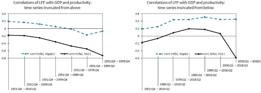
To understand the role of time in driving my correlation results, Figure 1 shows corre-lations between LFP and, alternatively, GDP and productivity across time by truncating these time series. The left panel of this …gure shows results from truncating the data from below, and reveals that given these truncations: the positive correlation of LFP with GDP holds across truncations; and the negative correlation of LFP with productivity is driven by the 1951 through 1969 period and the post 2010 period, which features a striking negative correlation. The right panel shows results from truncating the data from above, and reveals that given these truncations: the correlation of LFP with productivity is consistently neg-ative; and the positive correlation of LFP with GDP is driven by the 1951 through 1989 period. Taken together, the two panels in Figure 2 imply that the entirety of the time series

4_{This cyclical component is also obtained by, following Shimer (2005), and therefore using an HP …lter}

with smoothing parameter equal to 105

is important for characterizing the relationship between LFP, GDP, and productivity.

3

Behavior of LFP: Driving Forces

In order to shed light on the opposite signs of the correlation of LFP with GDP versus the correlation of LFP with productivity I examine the dynamic adjustment process of these variables given exogenous shocks to real economic activity using orthogonalized impulse response functions (IRFs). Then, using a forecast error variance decomposition (FEVD) I examine the importance the di¤erent variables used in equation (1) in driving the cyclical behavior of LFP. The recursive VAR framework that I use to obtain IRFs and the FEVD of LFP broadly follows, for ease of comparison with earlier literature, the recursive VAR framework of Fujita and Ramey (2007).

3.1

Impulse Response Functions

I …rst consider IRFs obtained from estimating equation (1). Rather than usingln (gdp=e)in this equation, I use, alternatively,ln (z)andln (gdp)in order to shed light on the correlations in Table 1. I henceforth refer to the analytical framework described by equation (1) using

ln (z) as the “productivity model.”5 _{Similarly, I refer to the analytical framework described}

by equation (1) usingln (gdp)as the “GDP model.”

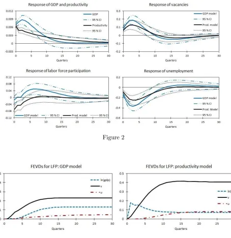
The left panel of Figure 2 shows IRF results from the GDP model given a one standard deviation unexpected and exogenous shock to GDP. The right panel of this …gure shows IRF results from the productivity model given a one standard deviation unexpected and exogenous shock to productivity.

Taken together, these two panels show that the responses of vacancies and unemploy-ment are very similar between models, both qualitatively and quantitatively (the substantial propagation of vacancies is in line with results from Fujita and Ramey, 2007). In contrast, the di¤erential adjustments of LFP, GDP, and productivity shown in Figure 2 explain the opposite correlations of LFP with, alternatively, GDP and productivity.

5_{Whenever using this model, in order to keepln (z) insulated from feedback e¤ects with other variables}

in the system I set A12(L) = 0,A13(L) = 0, and A14(L) = 0, whereAij(L) denotes the element in rowi

In the GDP model the response of LFP is hump shaped. On impact of the shock the response of LFP is nearly mute, but thereafter LFP rises above trend before beginning its return to trend only several quarters after the shock. Note that in this model the response of GDP is hump shaped as well. These hump shapes imply that after the shock there is a period over which LFP and GDP are rising simultaneously, which helps explain the positive correlation between these two variables.

Now, consider the productivity model. On impact of the shock productivity rises, but its response does not exhibit propagation. Neither does the response of LFP, which on impact of the shock jumps down and thereafter slowly returns to trend. The somewhat mirror-image responses of productivity and LFP to the shock explain these variables’ negative correlation. Next, to understand why, as shown in Table 1, LFP is positively correlated with vacan-cies and negatively correlated with unemployment despite its di¤erential adjustment in the GDP versus productivity models, consider the following. In the GDP model LFP begins rising above trend at the same time that vacancies are rising and unemployment is decreas-ing. Therefore, in the GDP model straightforward visual inference explains the positive correlation of LFP with vacancies and its negative correlation with unemployment.

However, in the productivity model signing the correlations of LFP with vacancies and unemployment on the basis of visual inference is more subtle. The key, though, lies in the fact that after the shock to productivity LFP starts moving back to trend immediately following its initial downward jump. Because LFP’s slow return to trend begins to take place immediately after the shock, LFP is rising (from below trend) at the same time that vacancies are rising and unemployment is decreasing. Therefore, LFP’s return to trend dominates the resulting sign of the correlation of LFP with vacancies and unemployment.

third of that of unemployment.

3.2

Forecast Error Variance Decomposition

Figure 3 presents a forecast error variance decomposition (FEVD) for LFP stemming from the VAR in equation (1) being run with, alternatively, GDP and productivity as the measure of real economic activity. This analysis helps understand the extent to which variables in the benchmark theory of equilibrium unemployment are important in driving the cyclical behavior of LFP. The left panel of this …gure shows results from the GDP model and the right panel shows results from the productivity model.

In each of these panels the value taken by a variable at a given point in time represents its contribution at that same point in time to the error associated with forecasting LFP. Intuitively, then, these plots explain how important any given variable is in explaining the behavior of LFP. For expositional simplicity these …gures do not show con…dence bands nor do they plot LFP’s forecast error variance stemming from itself (which at any given point in time is equal to the di¤erence between 1 and the values taken by the other variables plotted in each graph).

The left panel of Figure 3 shows that in explaining LFP at very short horizons the contri-butions of GDP, vacancies, and unemployment are negligible. Thereafter, all contricontri-butions rise, and in the medium to long run vacancies explain nearly a quarter of LFP—almost half of the proportion of LFP explained by LFP itself.

The right panel of this …gure shows that in explaining LFP at short horizons the con-tribution: of vacancies is fairly small; of unemployment is negligible; and of productivity is modest. Thereafter, the contribution of vacancies rises quickly and prominently, and in the medium to long run vacancies explain roughly 40 percent of LFP—about the same pro-portion of LFP explained by LFP itself. Over this same time horizon the contribution of unemployment rises modestly and plateaus.

4

Robustness

I examine the robustness of results pertaining to LFP by using two additional measures of real economic activity in the benchmark VAR, and also by estimating a smaller VAR.

Usingendogenousproductivity, that is,ln (gdp=e)as the VAR’s measure of real economic activity yields very similar results to those obtained from using exogenous productivity,

ln (z). In addition, using an exogenous measure of GDP per capita (constructed using similar methodology as that used to arrive at a measure of exogenous productivity) yields very similar results to those obtained from using (endogenous) GDP, ln (gdp).

In addition, I estimate a VAR with only two variables: LFP, and, alternatively, ln (z)

and ln (gdp). In these VARs I keep the variable and lag orders the same as in my main speci…cation. Given a shock to real economic activity results are nearly the same as those obtained from using my main speci…cation.

It follows that setting up the VAR guided by the underpinnings of the benchmark theory of equilibrium unemployment helps reveal the prominent role of vacancies in explaining LFP. However, the inclusion of vacancies and unemployment in the VAR is not crucial in itself for explaining the qualitatively di¤erent correlations of LFP with GDP and productivity.

All told, two consistent stylized facts emerge. First, in response to an exogenous shock to GDP, regardless of whether the measure of GDP is endogenous or exogenous, the on-impact response of LFP is nearly mute, and thereafter LFP exhibits a hump-shaped response. Second, given an exogenous shock to labor productivity, regardless of whether the measure of productivity is endogenous or exogenous, on impact LFP jumps down, and thereafter it slowly recovers without ever rising above trend.

5

Conclusions

alternatively, exogenous shocks to GDP and (labor) productivity. Important di¤erences in LFP’s adjustment depending on whether a shock to GDP or productivity takes place explain the opposite correlations of LFP with these variables.

My analytical framework is guided by the benchmark theory of equilibrium unemploy-ment. This guidance is important, as it helps reveal that job vacancies are a substantial factor driving the behavior of LFP. However, the inclusion of vacancies and unemployment in my main speci…cation (per the guidance of the benchmark theory of equilibrium unem-ployment) is not a fundamental force behind the di¤erent dynamic adjustment of LFP given exogenous shocks to, alternatively, GDP and productivity.

References

[1] Arseneau, D.M. and S.K. Chugh. 2012. “Tax smoothing in frictional labor markets.”

Journal of Political Economy, vol. 120 no. 5, pp.926-985.

[2] Campolmi, A. and Gnocchi, S., 2016. “Labor market participation, unemployment and monetary policy.”Journal of Monetary Economics, 79, pp.17-29.

[3] Elsby, M.W., Hobijn, B. and ¸Sahin, A., 2015. “On the importance of the participation margin for labor market ‡uctuations. Journal of Monetary Economics, 72, pp.64-82.” [4] Fujita, S., and G. Ramey. “Job matching and propagation.” Journal of Economic

Dy-namics and Control, vol. 31, no. 11, pp. 3671-3698.

[5] Krusell, P., Mukoyama, T., Rogerson, R. and ¸Sahin, A., 2012. “Is labor supply important for business cycles?” (No. w17779). National Bureau of Economic Research.

[6] Krusell, P., Mukoyama, T., Rogerson, R. and ¸Sahin, A. 2011.“ A three state model of worker ‡ows in general equilibrium.” Journal of Economic Theory, vol. 146, no. 3, pp.1107-1133.

[7] Pissarides, C.A. 2000. Equilibrium unemployment theory. MIT press.

[8] Shimer, R. 2005. “The cyclical behavior of equilibrium unemployment and vacancies.”

American Economic Review, vol. 95, no. 1, pp.25-49.

[9] Shimer, R. 2013. May. 10b. “Search, labor-force participation, and wage rigidities.” In

Advances in Economics and Econometrics: Volume 2, Applied Economics: Tenth World Congress, vol. 50, p. 197. Cambridge University Press.

[11] Tüzemen, Didem. 2017. “Labor market dynamics with endogenous labor force partici-pation and on-the-job search.”Journal of Economic Dynamics and Control, vol. 75, pp. 28–51.

[12] Van Zandweghe, W. 2012. “Interpreting the recent decline in labor force participation.” Federal Reserve Bank of Kansas City, Economic Review Article, …rst quarter.

[13] Veracierto, Marcelo. 2008. “On the cyclical behavior of employment, unemployment and labor force participation.” Journal of Monetary Economics, vol. 55, no. 6, pp. 1143–1157.

Table 1: U.S. quarterly labor market statistics 1951:Q4-2018:Q2

lf p u v ln (gdp) ln (z)

St. dev. 0.374 1.225 0.707 0.025 0.014 Autocorr. 0.873 0.953 0.945 0.939 0.889

lf p 1 – – – –

u -0.279 1 – – –

v 0.276 -0.823 1 – –

ln (gdp) 0.191 -0.856 0.797 1 –

ln (z) -0.177 -0.458 0.328 0.767 1

Figure 2