JHEP08(2017)124
Published for SISSA by SpringerReceived:May 16, 2017 Revised: August 3, 2017
Accepted: August 3, 2017
Published: August 28, 2017
Multi-soft gluon limits and extended current algebras
at null-infinity
Tristan McLoughlina and Dhritiman Nandanb,c,d aSchool of Mathematics, Trinity College Dublin,
College Green, Dublin 2, Ireland
bInstitut f¨ur Physik und IRIS Adlershof, Humboldt-Universit¨at zu Berlin,
Zum Großen Windkanal 6, 12489 Berlin, Germany
cInstitut f¨ur Mathematik und IRIS Adlershof, Humboldt-Universit¨at zu Berlin,
Zum Großen Windkanal 6, 12489 Berlin, Germany
dHiggs Centre for Theoretical Physics, School of Physics and Astronomy,
The University of Edinburgh, Edinburgh EH9 3JZ, Scotland, U.K.
E-mail: [email protected],[email protected]
Abstract:In this note we consider aspects of the current algebra interpretation of
multi-soft limits of tree-level gluon scattering amplitudes in four dimensions. Building on the relation between a positive helicity gluon soft-limit and the Ward identity for a level-zero Kac-Moody current, we use the double-soft limit to define the Sugawara energy-momentum tensor and, by using the triple- and quadruple-soft limits, show that it satisfies the correct OPEs for a CFT. We study the resulting Knizhnik-Zamolodchikov equations and show that they hold for positive helicity gluons in MHV amplitudes. Turning to the sub-leading soft-terms we define a one-parameter family of currents whose Ward identities corresponding to the universal tree-level sub-leading soft-behaviour. We compute the algebra of these cur-rents formed with the leading curcur-rents and amongst themselves. Finally, by parameterising the ambiguity in the double-soft limit for mixed helicities, we introduce a non-trivial OPE between the holomorphic and anti-holomorphic currents and study some of its implications.
Keywords: Scattering Amplitudes, Conformal and W Symmetry, Gauge Symmetry
JHEP08(2017)124
Contents1 Introduction 1
2 Soft limits for gluon amplitudes 4
2.1 Single-soft limits 4
2.2 Multi-soft limits 5
3 Current algebra interpretation of Yang-Mills soft limits 6
3.1 An su(N) current algebra 8
3.2 Sugawara construction for amplitudes 9
3.3 Energy-momentum tensor/current OPE 10
3.4 Energy-momentum OPE 11
3.5 Comments on a Knizhnik-Zamolodchikov equation 12
4 Sub-leading currents 15
4.1 Sub-leading algebra 16
5 Anti-holomorphic currents 19
5.1 OPE for anti-holomorphic currents 19
5.2 CFT interpretation of anti-holomorphic currents 22
1 Introduction
The simple geometric fact that a null vector in Minkowski space defines a point on the sphere at null infinity naturally suggests interpreting scattering amplitudes for massless particles as two-dimensional correlation functions. An early and prominent example of such an interpretation was given by Nair in [1] where certain N = 4 super-Yang-Mills (SYM) amplitudes were constructed using the operator product expansion (OPE) of the Kac-Moody currents which define a two-dimensional Wess-Zumino-Witten model. This construction in part lead to the development of the twistor string [2] which gives a complete description of tree-levelN = 4 SYM in terms of a two-dimensional world-sheet theory.
Kac-Moody structures have also recently appeared in the study of the soft-limits of gluon amplitudes [3,4]. Scattering amplitudes of massless particles such as gluons can be formally expanded in powers of a small scaling parameter δ multiplying the momentum of a particle which is thus taken to be soft, pµ=δ qµ, and which schematically gives
lim
δ→0An+1(δq) =
1
δ S
(0)(q) +S(1)(q)
An+O(δ), (1.1)
where An depends only on the remaining hard momenta. That scattering amplitudes of
JHEP08(2017)124
becomes soft has been long understood [5–8]. It is also known that at tree-level the be-haviour at the sub-leading order is universal, which is sometimes referred to as the Low theorem [5–7, 9–11], while for tree-level graviton amplitudes there is further universal behaviour at sub-sub-leading order [12]. Analogous sub-leading behaviour for gluon ampli-tudes has been recently studied [13–18]. In [4] He et al. showed that one could identify the tree-level leading soft theorem for positive helicity gluons with the Ward identity for holo-morphic two-dimensional Kac-Moody currents. These currents were shown to be related to the asymptotic symmetries of Yang-Mills theory given by large CPT-invariant gauge transformations [3].1 The OPE of the currents was extracted from the limit of two soft positive helicity gluons and it was shown that the level is zero in this identification, that is the algebra is a standard current algebra
Ja(z1)Jb(z2)∼
ifabcJc(z2) z12
. (1.2)
It was further noted that the limit where one positive and one negative helicity gluon are both taken soft is ambiguous with the result depending on the order in which the limit is taken. In [4] the authors gave the prescription of first taking all positive helicity gluons soft which resulted in one copy of the holomorphic Kac-Moody algebra but without a second anti-holomorphic copy arising from the negative helicity gluons.
Multi-soft limits of gluon amplitudes have been studied more generally in a number of recent works and universal behaviour in the limit where all gluons are taken soft simultane-ous was found for tree-level amplitudes using the BCFW [33] and CHY [34,35] formalisms in [36, 37]. These limits have also been studied using the CSW [38] formalism by [39] and by considering the field theory limit of string theory [40]. At leading order in the soft parameter this simultaneous double- and multi-soft limit differs from the consecutive case when there are particles of both positive and negative helicity. There is also universal behaviour in the sub-leading order of the multi-soft limit however the order in which the limit is taken is important even when all gluons have the same helicity.
We use these multi-soft limits to study further aspects of the current algebra interpre-tation in four dimensions. Starting with the leading soft-limit for positive helicity gluons we show that, by analogy with the Sugawara construction [41], one can use the double soft-limit to define a holomorphic energy-momentum tensor. Moreover we show, by analyzing the triple- and quadruple-soft limits of positive helicity gluons that this energy-momentum tensor has the standard OPE with both the holomorphic current and with itself. In a conformal field theory with a Kac-Moody symmetry the correlation functions of primary fields should satisfy certain differential equations, the Knizhnik-Zamolodchikov (KZ) equa-tions [42]. We consider the KZ equation for the amplitudes and show that while they hold for positive helicity gluons in MHV amplitudes this is not the case for the negative helicity gluons or for non-MHV amplitudes. While this suggests that the holomorphic currents do
1We focus entirely on gluon amplitudes but the relation between asymptotic symmetries and
JHEP08(2017)124
not provide a complete description of the putative CFT it motivates further analysing the sub-leading and negative helicity soft-limit.
We thus study the soft limit at sub-leading order and give these sub-leading soft-theorems an interpretation as Ward identities for two-dimensional currents which depend on a continuous parameter corresponding to the soft gluon energy, Jsuba (z;ωz). The OPE of these currents with themselves and with the leading order currents is then extracted from the sub-leading double-soft limits. As the algebra depends on exactly how the double soft limit is taken we introduce parameters to characterise this ambiguity. In the language of the two-dimensional field theory the leading terms of the OPEs are given by
Ja(z1)Jsubb (z2;ωz2)∼if
ab c
Jsubc (z2;ωz2)
z12
, (1.3)
Jsuba (z1;ωz1)J
b
sub(z2;ωz2)∼
ifabcJsubc (z2;css2 ωz1 +c
ss 1 ωz2)
z12 . (1.4)
As in [4] the anti-holomorphic currents are defined using the soft-limits of negative helicity gluons and to study the algebra with the holomorphic currents we consider double-soft limits involving both a positive and negative helicity gluon. However rather than picking a specific ordering of soft-limits we consider a linear combination and introduce variables with which we parameterise the ambiguity. The resulting algebra of currents is found to be
Ja(z1) ¯Jb(z2)∼ifabc
d1
¯
Jc(z 2) z12 −d2
Jc(z 2)
¯
z12 −d2 z12
¯
z12∂J c(z2)
. (1.5)
This OPE differs from the usual CFT chiral current algebra where one would find
Ja(z1) ¯Jb(z2) ∼ 0. However such OPEs can be considered in general [43] and bear re-semblance to the non-chiral current algebras that appear in the study of non linear sigma-models on super-group manifolds [44]. In the super-group case it is still possible to con-struct a holomorphic stress-energy tensor as the terms which would spoil conformality are removed by the fact that the Killing form is zero. While these theories are conformal they are however non-unitary and lack many of the features familiar from the study of two-dimensional CFTs (see [45] for a review of super-group CFTs). Of course there are a number of very significant differences between the current algebra in the super-group non-linear sigma-models and in our considerations, not least the absence of logarithmic terms, at least at tree-level, and naturally the Killing form for the gauge group in Yang-Mills theory is not usually taken to vanish as in the super-group case. To complete the algebra of currents we calculate the OPEs of the sub-leading currents with the anti-holomorphic currents and sub-leading anti-holomorphic coordinates
¯
Ja(z1)Jsubb (z2;ωz2)∼if
ab c
¯
Jsubc (z2;ωz2) ¯
z12
, (1.6)
Jsuba (z1;ωz1) ¯J
b
sub(z2;ωz2)∼if
ab c
Jsubc (z2;ds2ωz2) ¯
z12 −
¯
Jsubc (z2;ds1ωz1)
z12
+z12¯
z12
¯
∂J¯subc (z2;ds1ωz1) + 2
z12
¯
z12
∂Jsubc (z2;ds2ωz2)
JHEP08(2017)124
Using (1.5) one can compute the OPE of the anti-holomorphic currents with the holomor-phic stress-energy tensor. We do this in section5.2and show that it is consistent with the triple-soft limit involving two positive helicity gluons and one negative. Finally, using the leading order holomorphic and anti-holomorphic currents, we define a conjugation operator
C(z)∝:JaJ¯a: (z) and compute its OPE with the currents.
While we don’t attempt to give a more fundamental interpretation of these two-dimensional currents the renewed focus on understanding the asymptotic symmetries has lead to a number of interesting proposals for a holographic description of flat space scat-tering amplitudes. In [46], building on [47], a world-sheet theory with the null infinity boundary of flat space as its target space was proposed. An alternative approach based on the ambi-twistor string, [48,49], was studied in [50,51]. Recently, Cheung et al. [52] have proposed a holographic description which, following [53,54], makes use of a slicing of flat space into a family of AdS3 sub-spaces to interpret four-dimensional amplitudes in terms
of a two-dimensional CFT. They identify the conserved currents and energy-momentum tensor with the asymptotic symmetries of gluon and graviton amplitudes. While there are a number of differences with our current work, for example the central charge of the current algebra, it would be very interesting to understand better if there is a holographic interpretation of the sub-leading and anti-holomorphic currents.
2 Soft limits for gluon amplitudes
The central objects of our study are the soft limits of gluon scattering amplitudes. While we will be interested in the full colour dressed amplitudes it is convenient to start with colour stripped amplitudes. Consider ann+1-leg amplitude where we take the first leg to be a soft particle of helicityhq with momentumδq, or in terms of spinor variables, {
√
δλq,
√
δ˜λq}.2
The soft limit corresponds to expanding the amplitude in powers of δ1 and we keep only those terms in the expansion which are universal. As it will make subsequent formulae simpler we will often simply denote the non-soft legs with momenta pi, i = 1, . . . , n by
1,2, . . . , n.
2.1 Single-soft limits
The single-soft limits for gluon amplitudes were found, up to the first sub-leading term, in [7,9,13]
An+1(δ1qhq,1, . . . , n)→
1
δ1
Sn,1(0)(qhq) +S(1) n,1(q
hq)
An(1, . . . , n) (2.1)
where, for a positive helicity gluon, hq = +, between neighboring particles n and 1, the
universal soft-factors can be written using the spinor-helicity formalism as
Sn,1(0)(q+) = hn1i
hn qihq1i, S
(1) n,1(q
+) = 1
hq1iλ˜
˙ α q
∂ ∂˜λα˙
1
+ 1
hn qi˜λ
˙ α q
∂ ∂λ˜α˙
n
. (2.2)
JHEP08(2017)124
Here we use the conventions
habi=αβλαaλ β
b =λaβλ β b =−λ
α
aλbα (2.3)
and similarly for the dotted indices, [ab] = α˙β˙˜λαa˙λ˜ ˙ β
b. Correspondingly we will write the
contraction of a spinor with a derivative as
˜
λαa˙ ∂
∂˜λαb˙ =−[a
¯
∂b]. (2.4)
For a negative helicity gluon the soft factors are given by conjugation of the spinor variables,
λi↔λ˜i.
2.2 Multi-soft limits
One can similarly consider the limit of gluon amplitudes with multiple soft gluons. However as mentioned there is in general an ambiguity in the result which depends on the order in which the gluons are taken to be soft. Starting with the case of two soft gluons we consider then+2-leg amplitude where we will take the first and second legs to be soft particles with helicities hq1 and hq2 and momenta {
√
δ1λq1,
√
δ1λ˜q1} and {
√
δ2λq2,
√
δ2λ˜q2} respectively. In particular, if one takes the gluons soft sequentially we call this a consecutive soft limit in contradistinction to the simultaneous or double soft limit. These consecutive soft limits can be calculated straightforwardly from repeated action of the above single soft factors.
We define the consecutive soft factor, CSLn,1(q hq1 1 , q
hq2
2 ), to be
CSLn,1(q hq1 1 , q
hq2
2 )An(1, . . . , n)≡ lim δ2→0
lim
δ1→0
An+2(δ1qhq1
1 , δ2q hq2
2 ,1. . . , n) (2.5)
= 1 δ1S (0) n,q2
qhq1
1
+Sn,q(1)2
qhq1
1 1 δ2S (0) n,1
qhq2
2
+Sn,1(1)
qhq2
2
An(1, . . . , n) ,
where we take the particle q1 soft first and then q2. As it will be of interest later, let us
give the explicit expression:
CSLn,1(q1+, q+2) =
1
δ1δ2
hn1i
hnq1ihq1q2ihq21i +O(δ
0
2/δ1, δ01/δ2). (2.6)
If we take the reverse consecutive limit, i.e. take leg q1 soft and then leg q2, the leading
term in CSL(q1+, q2+) is unchanged. However when the particles have different helicity, or when we extract sub-leading multi-soft terms, the order of limits will be important and so we consider linear combinations by defining more general multi-soft limits
lim
α ≡
α12...m lim δm→0
. . . lim
δ2→0 lim
δ1→0
+α21...m lim δm→0
. . . lim
δ1→0 lim
δ2→0 +. . .
(2.7)
with the ellipses denoting all further permutations. Thus we can define a multi-parameter family of consecutive soft limits
αCSLn,1
1hq1,2hq2, . . . , mhqmA
n(1, . . . , n) = lim α An+m
δ1q hq1
1 , . . . , δmq hqm
m ,1, . . . , n
.
JHEP08(2017)124
The effect of this general limit can be seen in the sub-leading term in the expansion of two soft, positive helicity gluons which a short calculation shows is given by
lim
α An+2 δ1q +
1, δ2q2+, . . .
sub−leading =
1
δ1
α12hnq2ihq11i+α21hn1ihq1q2i hq1q2ihq11ihnq1ihq21i
[q2∂1]
+α12
δ1
[q2∂n]
hnq1ihq1q2i
+ 1
δ2
α12hn1ihq1q2i+α21hq11ihnq2i hq1q2ihnq2ihnq1ihq21i
[q1∂n] +α21
δ2
[q1∂1]
hq21ihq1q2i
An.
(2.9)
It is perhaps worthwhile to note that this expression is only valid for generic external momenta as we have neglected holomorphic anomaly terms that can arise when external legs are collinear with soft legs, however it will turn out that they are not necessary for our considerations.
For the case of mixed helicity the two orderings of limits already differ at leading order in the soft expansion and so we can define a two parameter double-soft limit
αCSL(0)n,1(q1+, q2−) = 1
hnq1i[q21]
α21
hn1i
[q1q2] [q11]
hq11i+α12
[n1]
hq1q2i hq2ni
[q2n]
, (2.10)
where αCSL(0) has the overall (δ1δ2)−1 dependence stripped off. As described previously, we can of course also consider the simultaneous double-soft limit where both particles are taken soft together. The case of two gluons of the same helicity is identical to the consecutive limit but the case of one negative helicity and one positive is different. In four space-time dimensions the leading order double-soft mixed helicity factor is given in the spinor helicity formalism by
DSL(0)n,1(q+1, q2−) = 1
hn|q12|1]
1 2pn·q12
[n1]hnq2i3
hq1q2ihnq1i −
1 2p1·q12
hn1i[1q1]3 [q1q2][q21]
, (2.11)
where
q12:=q1+q2. (2.12)
This expression differs from the consecutive limit due to the sum of soft momenta in the denominator but it is closest to the symmetric α12 = α21 = 12 case. A similar ambiguity
appears at sub-leading order when we consider the double-soft limit in the mixed helicity case. Explicit formulae can be found in [36] but in this case we will focus on the consecutive limits which can be calculated by repeated use of the single-soft limits (2.2).
3 Current algebra interpretation of Yang-Mills soft limits
Let us consider the single and double soft limits of Yang-Mills amplitudes but now instead of just focussing on colour-ordered partial amplitudes we examine the full amplitude
An({pi, hi, ai}) =gYMn−2
X
σ∈Sn/Zn
An(σ1, . . . , σn)Tr(Taσ1 . . . Taσn) (3.1)
where the sum runs over all permutations, Sn, modulo those which are cyclic, Zn, and Ta
JHEP08(2017)124
−→
[image:8.595.165.411.84.216.2]−→
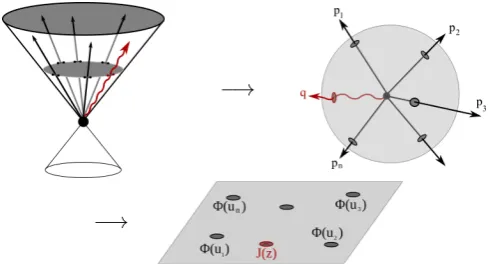
Figure 1. The gluons emerging from the amplitude travel on the light-cone and intersect with the sphere at null infinity, or any finite time representation, at points which can be given complex coordinates z, for the soft gluon, and ui for the hard gluons. The soft gluon is then interpreted as the insertion of a current operator at the point z while the ui denote the insertion points of additional fields.
factors ofgYMbut as we are only concerned with tree-level amplitudes they can be trivially
restored. If we take the soft-limit of then+ 1-particle amplitude we have at leading order in the soft-expansion
lim
δ→0An+1(δq1, hq1, a;{pi, hi, ai})
1
δ
= X
σ∈Sn
1
δS (0) σn,σ1
qhq1
1
An(σ1, . . . , σn)Tr(TaTaσ1. . . Taσn).
We can rewrite this soft limit in terms of two-dimensional position space variables by using the parameterisation for the soft-gluon momentum
λq1 =
√
ω(1, z), λ˜q1 =
√
ω(1,z¯), (3.2)
and for the hard momenta the parameterisation λi = √νi(1, ui) and ¯λi = √νi(1,ui¯). Essentially the complex z-variable describes the position of the intersection of the soft gluon’s trajectory with the sphere at asymptotic infinity and theui’s are the corresponding
intersection points for the hard gluons, see figure 1. We take all gluons to be outgoing and so this is in fact the anti-sky mapping. In these variables we have for the leading single soft factor (2.2) ,
(−δω)Si,j(0)(q+1) = 1
z−uj −
1
z−ui, (3.3)
where we see that it has simple poles as the soft momenta approach the hard momentum in position space i.e. z→ui for each i. Now we define,
Ja(z)· An({ui,ui, νi¯ })≡ −lim
δ→0(δω)An+1(δp,+, a;{pi, hi, ai}), (3.4)
and so
Ja(z)· An({ui,u¯i}) = n
X
`=1
h 1
z−u`
i X
˜ σ∈Sn−1
An(`,σ˜2, . . . ,σ˜n)Tr([Ta, Ta`]Ta˜σ2 . . . Taσn˜ )
=
n
X
`=1 T`a z−u`
JHEP08(2017)124
where in the last line T`a is understood to act (in the adjoint representation) only on the
`-th particle colour factor inAn. This is the result of He et al. [4] who compared it to the
OPE for a Kac-Moody currentJa and a primary field in a representation R
Ja(z)ΦrR(u)∼ (T
a
R)rsΦsR(u)
z−u (3.6)
and the consequent Ward Identity
hJa(z)ΦR1(u1,u¯1). . .ΦRn(un,u¯n)i= n
X
`=1 TRa
`
z−u`hΦR1(u1,u¯1). . .ΦRn(un,u¯n)i. (3.7)
Note that we use the notation Ja in (3.5) to denote the expression derived from a
four-dimensional scattering amplitude perspective and the Ja in (3.7) to be the corresponding quantity from the two dimensional CFT perspective. It is the formal similarity of these two expressions that suggests the interpretation of the soft-gluon limits as corresponding to the insertion of the current operator and it is interesting to ask to what extent this analogy can be extended.
3.1 An su(N) current algebra
As a first step, it is natural to ask whether one can reproduce the current-current OPE
Ja(z1)Jb(z2)∼
kδab
(z1−z2)2
+ if
ab
cJc(z2) z1−z2
. (3.8)
At the level of correlation functions we would expect to find,
hJa(z1)Jb(z2)Φ(u1). . .i ∼
kδab
(z1−z2)2hΦ(u1). . .i+ ifabc z1−z2
X
` T`c
z2−u`hΦ(u1). . .i. (3.9)
That the corresponding result can be found by analyzing the double-soft limits of ampli-tudes was shown in [4] and as it is useful for our later results we rederive this fact in our notations. To this end we consider the double soft limit which we can write as
lim
δ→0An+2(δ1q1, hq1, aq1;δ2q2, hq2, aq2;{pi, hi, ai}) =
X
σ∈Sn
(CSLσn,σ1(q
hq1 1 , q
hq2
2 ) +CSLσn,σ1(q
hq2 2 , q
hq1
1 ))Tr(q1q2σ1. . . σn)
n
X
i=2
Sσn,σ1(q
hq1
1 )Sσi−1,σi(q hq2
2 )Tr(q1σ1. . . σi−1q2σi. . . σn)
iCSLσn,σ1(q
hq2
2 , q hq1
1 )faq2aq1c Tr(cσ1. . . σn)
An(σ1, . . . , σn) (3.10)
in a slightly condensed notation with Tr(q1q2σ1. . . σn) = Tr(Taq1Taq2Taσ1. . . Taσn) etc. As
JHEP08(2017)124
order of limits is not relevant and so we simply take the simultaneous limit with a single soft parameter δ1 =δ2 =δ. We use the identity for consecutive soft-limits
CSL(0)σn,σ1
qhq1
1 , q hq2 2
+CSL(0)σn,σ1
qhq2
2 , q hq1 1
=Sσ(0)n,σ1
qhq1
1
Sσ(0)n,σ1
qhq2
2
(3.11)
here with both helicities positivehq1 =hq2 = +, and so we can combine the first two terms to find
lim
δ→0An+2(δq1,+, aq1;δq2,+, aq2;{pi, hi, ai}) =
X
σ∈Sn ( n
X
i=1
Sσ(0)n,σ1(q1+)Sσ(0)i−1,σi(q2+)Tr(q1σ1. . . σi−1q2σi. . . σn)
+iCSL(0)σn,σ1(q2+, q1+)faq2aq1
c Tr(cσ1. . . σn)
)
An(σ1, . . . , σn). (3.12)
Re-writing the soft-factors in terms of polarisation vectors one recovers the result quoted in [4].
The singularities of these double soft factors in the collinear limit, as the soft momenta approach each other, can be made clear by rewriting them in position space and examining thez1 →z2 limit. We can see that there will be no singularities from the terms involving the products of single soft factors; these terms instead give poles when the soft momenta
approach the hard momenta. However the term involving the consecutive double soft
limit does have such a singularity and gives rise to the non-trivial algebra between the holomorphic currents. More explicitly, defining
Ja(z1)Jb(z2)· An({ui,u¯i})≡ lim δ→0(4δ
2 ω
z1ωz2)An+2(δq1,+, a;δq2,+, b;{pi, hi, ai}) (3.13) we find
Ja(z
1)Jb(z2)· An({ui,u¯i})∼
1
z1−z2 n
X
`6=m=1
X
σ∈Sn−2
ifbac
1
z2−u` −
1
z2−um
×Tr(`cmσ1. . .)An(`mσ1. . .)
= if
ba c z1−z2
n
X
`=1
1
z2−u`
X
˜ σ∈Sn−1
Tr([`, c]˜σ1. . .)An(`σ˜1. . .)
= if
ab c z1−z2
n
X
`=1 T`c z2−u`
An({ui,ui¯ }). (3.14)
Hence comparing with (3.9) we see that the double soft-limit reproduces the structure of level-zero Kac-Moody or simply a current algebra as described in [4].
3.2 Sugawara construction for amplitudes
If this is a correct interpretation, i.e. there is a level-zero Kac-Moody symmetry acting on amplitudes, we may try to construct a holomorphic energy-momentum tensor via the Sugawara construction. Namely, we define
TS(z1) =γ :JaJa(z1) : ≡γ lim z2→z1
JHEP08(2017)124
whereγ is a constant related to the dual Coxeter number,h∨, byγ = 2h1∨, and the normal
ordering is missing the usual singular term that occurs in the Kac-Moody case as the current algebra has no central extension. At the level of correlation functions this leads us to again consider double insertions of holomorphic currents and so, as the analogue for amplitudes is the double soft limit, we again consider (3.13) but now with contracted adjoint indices. That is we define
TS(z1) = 1 2h∨ zlim
2→z1
JaJa(z1). (3.16)
We could in principle work with a general Lie group but for simplicity we focus on the case of su(N) colour where we can contract the indicesaand busing the identity
(Ta)ij(Ta)kl=δilδ j k−
1
Nδ j
iδlk. (3.17)
and in this caseh∨ =N.
To calculate the scattering amplitude analogue of the insertion of an energy-momentum tensor into a correlation function we consider the singularities as either of the soft momenta approach one of the hard momenta, say um, and then expand the z2 dependence near z1.
Using the notation z1m=z1−um form= 1, . . . , n we write the result
TS(z
1)· An({ui,u¯i}) ≡
1 2NJ
a(z
1)Ja(z1)· An({ui,u¯i})
=
n
X
m=1
X
σ∈Sn−1
n 1
2N
1
z1m n−1
X
i=1
1
z1σi
Tr([a, m]σ1. . .[a, σi]. . .)
+ 1
z1m2 Tr(mσ1. . .)
o
An(mσ1. . .). (3.18)
While this definition seems sensible we should ask whether it satisfies the basic properties of a energy-momentum tensor for a conformal field theory.
3.3 Energy-momentum tensor/current OPE
In two-dimensional conformal field theory a defining characteristic of TS(z1) is its OPE
with the holomorphic current operator
TS(z1)Ja(z3)∼ J
a(z3) z2
13
+∂J
a(z3) z13
. (3.19)
The analogous object for the amplitude is a specific case of the triple soft-limit
lim
δ→0An+3(δq1, hq1, aq1;δq2, hq2, aq2;δq3, hq3, aq3;{pi, hi, ai}) (3.20)
= X
σ∈Sn nnX−1
s=1 n
X
r=1 r6=s
Sσ(0)n,σ1(qhq1
1 )S(0)σs,σs+1(q
hq2
2 )Sσ(0)r,σr+1(q
hq3
3 )Tr(q1. . . σsq2. . . σrq3. . .)
+
n−1
X
r=1
(CSL(0)σn,σ1(qhq1
1 , q hq2
2 ,) +CSL (0) σn,σ1(q
hq2 2 , q
hq1 1 ))S
(0) σr,σr+1(q
hq3
3 ) Tr(q1q2. . . σrq3. . .)
+iCSL(0)σn,σ1(qhq2
2 , q hq1
1 )S (0) σr,σr+1(q
hq3
3 )f
aq2aq1cTr(c . . . σrq3. . .) + (q2 ↔q3) + (q1 ↔q3)
+CSL(0)σn,σ1(1
h1,2h2,3h3)Tr(123σ
1. . . σn) + perm(1,2,3)
o
JHEP08(2017)124
We take all gluons to have positive helicity, such that the triple and double soft limits are the same regardless of whether we take the consecutive or simultaneous soft limit and so, as in the double-soft case, we set all soft parameters equal. The product of three holomorphic currents is then defined to be
Ja(z1)Jb(z2)Jc(z3)· An({ui,ui¯}) ≡ (3.21)
−lim
δ→0(δ 2 ωz
1ωz2ωz3)An+3(δq1,+, a, δq2,+, b, δq3,+, c;{pi, hi, ai}).
In the standard two-dimensional conformal field theory calculation, to compute the OPE of the energy-momentum tensor with the current operator we collect the terms which are singular as z3 approaches either z1 orz2. In the soft-limit such terms correspond to the soft momentumq3 becoming collinear with either q1 orq2. In particular the contributions
from the triple soft terms split into two groups, those where the soft particles q1 andq2 are
adjacent which come with a colour factor (N−N1)Tr(cσ1. . . σn) and those whereq1 and q2
are split by particleq3 which have (−N1)Tr(cσ1. . . σn). Combining these terms we find that
the (−N1) factors cancel. There are further contributions from terms involving double soft limits times single soft factors which have colour structures fcadTr(a . . . σrd . . .) however
these terms cancel between themselves. This makes use of the identity (3.11) as well as the fact that
Tr(TaTaσ1 . . . Taσr[Tc, Ta]. . .) + Tr([Tc, Ta]Taσ1. . . TaσrTa. . .) = 0. (3.22)
Following the conformal field theory calculation, we then expand this in powers of z21 = z2−z1 and keep the leading term (in principle there could be a more singular term however
this term is absent which corresponds to the level of the current algebra being zero ). We finally have
TS(z1)Jc(z3)· An({ui,ui¯ }) ∼
1
z231
X
σ∈Sn
1
z1−uσ1
− 1
z1−uσn
Tr(cσ1. . . σn)An(σ1. . . σn)
= 1
z2 31
n
X
`=1
1
z1−u`
X
˜ σ∈Sn−1
Tr([c, `]˜σ1. . .)An(`σ1˜ . . .)
= 1
z2 31
Jc(z1)· An({ui,ui¯ }) (3.23)
which after expanding thez1 dependence on the right hand side is the required result.
3.4 Energy-momentum OPE
Using the OPE of holomorphic currents it can be shown that the Sugawara energy-momentum tensor for a current algebra (k= 0) satisfies the OPE
T(z1)T(z3)∼
2T(z3)
(z1−z3)2
+ ∂T(z3) (z1−z3)
JHEP08(2017)124
and so defines a conformal field theory with vanishing central charge. Correspondingly, inserted into a correlator of primary fields Φ(ui), we have that
hT(z1)T(z3)Φ(u1). . .Φ(un)i=
2 (z1−z3)2+
∂z3
(z1−z3) (3.25)
+
n
X
i=1
∆ (z1−ui)2
+ ∂ui
(z1−ui)
×hT(z3)Φ(u1). . .Φ(un)i.
In terms of the soft-limits of amplitudes this Ward identity should be reproduced by the collinear part of the quadruple soft limit for positive helicity gluons. Once again as we are only considering positive helicity gluons there is no ambiguity in the order of limits. In the two-dimensional conformal field theory construction one starts with pairs of currents,
Ja1(z1)Ja2(z2) and Ja3(z3)Ja4(z4), and to calculate the OPE one first extracts the terms which become singular as either z1 or z2 approaches either z3 or z4 and then takes the
limits z2 →z1 and z4 →z3. For the amplitude one similarly considers those terms which are singular as either q1 or q2 become collinear with q3 or q4. The singular terms get
contributions from quadruple soft terms, where all soft particles are adjacent, from triple-soft terms and from the “double” double-triple-soft terms. Carefully combining all these terms we find, after taking the z2 →z1 limit, that the singular terms in the quadruple soft limit are
TS(z1)TS(z3)·A ≡lim
δ→0
(Q4
i=1ωzi)
(2N)2 An+4(δq1,+, a;δq1,+, a;δq3,+, b;δq3,+, b;{pi, hi, ai})
∼ 2
z132 (2N)
X
σ∈Sn n
X
i=1
uσn−uσ1 (z3−uσn)(z3−uσ1)
uσi−1−uσi
(z1−uσi−1)(z1−uσi)
Tr(aσ1. . . aσi. . .)An.
This can be compared with the definition of a single insertion of the energy-momentum tensor in (3.18) and, after further expanding the z1 dependence near z3, we see that we indeed reproduce the OPE in (3.24) as expected.
While we restrict our considerations to gluon amplitudes it is interesting to note that the sub-leading soft theorem for a graviton has been identified with the Ward identity for a two-dimensional energy-momentum tensor [58] which suggests interpreting the collinear limit of double-soft gluons as a graviton. This is reminiscent of recent work [59–62] showing that amplitudes describing the interactions of gravitons with gluons can be written as linear combinations of amplitudes in which the graviton is replaced by a pair of collinear gluons.
3.5 Comments on a Knizhnik-Zamolodchikov equation
Given the above construction for the energy-momentum tensor it is interesting to ask if we can derive conformal Ward identities by considering correlation functions with insertions of the energy-momentum tensor. However, a priori, even if there is a sensible conformal field theory interpretation of the asymptotic states the current algebra may only form part of it, which is to say the full energy-momentum tensorT(z) would be given by
JHEP08(2017)124
If we consider the individual terms in the mode expansion
( ˆL−nΦ)(u) =
I dz
2πi
1
(z−u)n−1T(z)Φ(u),
( ˆJ−anΦ)(u) =
I dz
2πi
1 (z−u)nJ
a(z)Φ(u) (3.27)
we have that
ˆ
L−m = ˆL0−m+γ
X
l≤−1
ˆ
JlaJˆma−l+γ X l>−1
ˆ
Jma−lJˆ−al. (3.28)
In conformal field theory we can insert this inside a correlation function of primary fields and if we consider the case whereT0(z) is absent we can derive the Knizhnik-Zamolodchikov equation
hΦ(u1). . .( ˆL−1Φ)(um). . .Φ(un)i=
hΦ(u1). . .
γ( X
l≤−1
ˆ
JlaJˆ−al−1+ X
l>−1
ˆ
J−al−1Jˆ−al)Φ
(um). . .Φ(un)i.
Turning now to the scattering amplitudes, we consider the individual terms in the ex-pression for an insertion of the energy-momentum tensor following from the double-soft limit, (3.18). We have at leading order
I
Cum dz1
2πi z1mT S(z
1)· An({ui,u¯i}) =An({ui,u¯i}) (3.29)
where Cum is a contour surrounding the point um. This has the expected form for an
insertion of the energy-momentum tensor into a correlation function of primary fields with weight one. More non-trivially the sub-leading term is given by
I
Cum
dz1
2πi T S(z
1)· An({ui,u¯i}) =
1
N n
X
`=1 `6=m
Tma ⊗T`a um−u`
An({ui,u¯i}). (3.30)
The usual conformal Ward identity would then imply
∂umAn({ui,ui¯}) =L 0
−1· An({ui,ui¯ }) +
1
N n
X
`=1 `6=m
Tma ⊗T`a um−u`
An({ui,ui¯}) (3.31)
whereL0−1 is the residue ofT0(z1) at z1 =um. It is tempting to ask what would happen if
theL0
−1 term would be absent, that is, if the current algebra described the complete CFT.
As an example one can consider the MHV amplitudes. It is useful to define a rescaled quantityGn as follows
Gn({ui,ui, hi¯ }) =
n
Y
`=1 νh`
JHEP08(2017)124
In the simplest three-particle case
GMHV3 (1−,2−,3+) = (u1−u2)
3
(u2−u3)(u3−u1)
(Tr(Ta1Ta2Ta3)−Tr(Ta1Ta3Ta2)) (3.33)
and it is immediately obvious that (3.31) withL0−1 absent is satisfied for u3 but notu1 or
u2. In fact it is easy to check explicitly that the KZ-equation with L0−1 absent continues
to hold for the positive helicity gluons in higher point MHV amplitudes (currently done with Mathematica to seven-points). It is slightly non-trivial to check that the double trace terms, which arise whenmand`in (3.31) are not adjacent in a specific colour-ordered term, vanish. This requires that the colour ordered amplitudes satisfy a number of identities. For example, for them = 3 KZ equation one such relation at four points is the vanishing of the Tr(Ta1Ta4)Tr(Ta2Ta3) double-trace terms, which requires that
A(1,2,3,4)
u3−u1 +
A(1,4,3,2)
u3−u1 −
A(1,2,3,4)
u3−u2 −
A(1,3,2,4)
u3−u2
−A(1,4,2,3)
u3−u2 −
A(1,4,3,2)
u3−u2 +
A(1,3,2,4)
u3−u4 +
A(1,4,2,3)
u3−u4 = 0. (3.34)
More generally for them-th KZ-equation the vanishing of the
Tr(TamTaσ1. . . Taσ`−1)Tr(Taσ` . . . Taσn−1) (3.35)
term requires
X
cyc{σ`,...,σn−1}
1
um−uσ` −
1
um−uσ`−1
An(mσ1. . . σ`. . . σn−1)
−
1
um−uσ1
− 1
um−uσn−1
An(m, σ`. . . σn−1σ1. . . σ`−1)
= 0 (3.36)
where cyc{σ`, . . . , σn−1}denotes the sum over all cyclic permutations. We checked all such
identities hold up to seven points for MHV amplitudes. However, starting with the six-point NMHV amplitude it no longer appears that the KZ equations holds even for the positive helicity gluons. This suggests, unsurprisingly, that if there is a CFT interpretation there is additional structure and as there is further universal behaviour in the soft-limits we attempt to also interpret these in the context of a two-dimensional description.
Let us round off this section with an interesting connection of the above amplitude relations with the so called Bern-Carrasco-Johansson (BCJ) [63] relations resulting from the color-kinematic duality of gauge theory amplitudes. We can re-write the previous example of the four point amplitude relation (3.34) in a different way using Kleiss-Kuiff and the photon decoupling relations, which gives A(1,2,3,4) =A(1,4,3,2) and A(1,3,2,4) =
A(1,4,2,3). Using these relations we can rewrite the left-hand side of (3.34) as,
A(1,2,3,4)
1
u31
− 1
u32
+A(1,4,2,3)
1
u34
− 1
u32
= 0
A(1,2,3,4)u12
u31 +A(1,4,2,3) u42
JHEP08(2017)124
Now using the representations of the spinor helicity variables hiji = √νiνjuij and [ij] =
√
νiνjuij¯ and four-point momentum conservation we get,
u12u34 u31u24
= h12ih34i[12]
h24ih31i[12] =
s12 s24
, (3.38)
where sij = (pi+pj)2 are the Mandelstam invariants. Hence, using these change of vari-ables (3.37) and resultantly (3.34) becomes,
A(1,2,3,4)s12=s13A(1,4,2,3), (3.39)
which is remarkably the 4−point BCJ relation. Thus the MHV amplitude relation derived from demanding the vanishing of the double-trace terms in our KZ equations leads to the BCJ relation at least for 4 points. This connection is harder to see for higher number of points and we will report on this in a future publication.
4 Sub-leading currents
So far we have only been considering the leading soft terms, however it is known that the sub-leading soft terms for Yang-Mills amplitudes are also universal. This behaviour, the gluon version of the Low theorem [5–7, 9–11] described in section 2.1, is understood to be valid only at tree-level and for generic configurations of the remaining external hard legs [17]. We will only consider such configurations and so neglect boundary terms in the kinematic space where additional particles become collinear. At loop level such corrections could no longer be avoided and so it would be interesting to carefully understand these terms, and more generally to make contact with the SCET [64–67] description used in [17]. We thus repeat the above analysis at the sub-leading order by defining the sub-leading currents, Ja
sub, as
Jsuba (z;ωz)· An({ui,u¯i, νi})≡ −lim
δ→0(1 +δ∂δ)ωzAn+1(δq,+, a;{pi, hi, ai}) (4.1)
where the (1 +δ∂δ) factor picks out the sub-leading soft term. We have that
Jsuba (z;ωz)· An({ui,ui, νi¯ }) = n
X
`=1
ωz∂ν`+ ωz
ν`(¯z−u`¯ ) ¯∂`
T`a z−u`
An({ui,ui, νi¯ }) (4.2)
where ¯∂` = ∂¯∂z` and ∂ω` = ∂
∂ω`. If we again attempt to interpret this in terms of the OPE
of a current with a primary field we must consider the primary fields as depending on an auxiliary variable ν and we have
Jsuba (z;ω)ΦRr(w;ν)∼ (T
a R)rs
ω∂ν +ων(¯z−u¯) ¯∂ΦsR(w;ν)
z−u . (4.3)
JHEP08(2017)124
algebra in the principle continuous series representations, Φj,`(w), for which we introduce the complex parameter x, and the OPE is given by
J3(z)Φj,`(w;x)∼ t
3Φj,`(w;x) z−u +
k`
2 Φ
j,`(w;x) (4.4)
where t3 =x∂x∂ . In the case at hand we see that, in addition to having a one-parameter family of such currents, there is no extension as k = 0. Adamo and Casali [46] have, in their world-sheet theory with null infinity as its target space, given the definition of a charge with reproduces the sub-leading soft factor. It would be interesting to understand if there is a relation between the currents introduced here and their charges which have the interpretation as rotating the space of null generators. It is also known that these sub-leading soft terms in four-dimensions are intimately connected to the conformal invariance of the theory [17].
4.1 Sub-leading algebra
To continue the two-dimensional interpretation of the collinear soft limits to sub-leading order and given these new currents we analyse the algebra that they form with the leading currents and amongst themselves.
JsubJ. To find the OPE of the Kac-Moody currentJa(z) with Jsuba (z) we must consider
part of the double soft limit at sub-leading order. The order of limits in this case is relevant and a specific prescription must be given with the results dependent on the prescription. We start with the consecutive limit and take leg q2 soft before leg q1:
lim
δ1→0 lim
δ2→0
(1 +δ1∂δ1)δ2An+2(δ1q1, hq1, aq1;δ2q2, hq2, aq2;{pi, hi, ai}) =
X
σ∈Sn nh
Sq(0)1,σ1(qhq2
2 )S (1) σn,σ1(q
hq1 1 ) +S
(0) σn,q1(q
hq2 2 )S
(1) σn,σ1(q
hq1 1 )
i
Tr(q1q2σ1. . . σn)
+
n
X
i=2
Sσ(0)i−1,σi(qhq2
2 )Sσ(1)n,σ1(q
hq1
1 )Tr(q1σ1. . . σi−1q2σi. . . σn)
+iSσ(0)n,q1(qhq2
2 )Sσ(1)n,σ1(q
hq1
1 )faq2aq1c Tr(cσ1. . . σn)
o
An(σ1, . . . , σn). (4.5)
An important feature of this formula is that, as previously, the singularities as q1 and q2
become collinear only occur in the third set of terms on the right-hand side as those that appear in the first set of terms cancel amongst themselves
lim
δ1→0 lim
δ2→0
(1 +δ1∂δ1)δ2An+2(δ1q1, hq1, aq1;δ2q2, hq2, aq2;{pi, hi, ai}) =
− X
σ∈Sn
h hσnσ1i
hσnq2ihq2σ1i
[q1∂¯σ1]
hq1σ1i +
[q1∂¯σn]
hσnq1i
i
Tr(q1q2σ1. . . σn) (4.6)
+. . .
+i hσnq1i
hσnq2ihq2q1i
[q1∂σ¯ 1]
hq1σ1i
+[q1∂σ¯ n]
hσnq1i
faq2aq1
c Tr(cσ1. . . σn)
JHEP08(2017)124
Using the coordinate representation (3.2) we can find the most singular part asz1 →z2
lim
δ1→0 lim
δ2→0
(1 +δ1∂δ1)δ2ωz1ωz2An+2 ∼
ifaq1aq2c
z12 n
X
`=1
"
T`cωz1(∂ν`+ ¯ z2−¯u`
ν`
¯
∂`) z2−u`
#
An. (4.7)
If we had instead takenδ2 to zero afterδ1 we would find
lim
δ2→0 lim
δ1→0
(1 +δ1∂δ1)δ2An+2(δ1q1, hq1, aq1;δ2q2, hq2, aq2;{pi, hi, ai}) =
X
σ∈Sn nh
Sσ(1)n,q2(qhq1
1 )Sσ(0)n,σ1(q
hq2
2 ) +Sq(1)2,σ1(q
hq1
1 )Sσ(0)n,σ1(q
hq2 2 )
i
Tr(q1q2σ1. . . σn)
+· · ·+iSq(1)2,σ1(qhq1
1 )S (0) σn,σ1(q
hq2 2 )f
aq2aq1
c Tr(cσ1. . . σn)
o
An(σ1, . . . , σn). (4.8)
Again one can show that in the collinear limit the potentially singular terms only come from the last line above, however in this case there are in fact no non-vanishing singular terms in the collinear limit. Such terms potentially could have arisen from the holomorphic anomaly
∂ ∂λ¯a˙
1
hλµi =πa˙b˙µ¯ ˙
bδ(2)(hλµi) (4.9)
which gives
lim
δ2→0 lim
δ1→0
(1 +δ1∂δ1)δ2An+2=
− X
σ∈Sn
· · ·+iπfaq2aq1 c
hσnσ1i
hq2q1i
−[q1σn] hq2σ1iδ
(2)(hσ nq2i)
+[q1σ1]
hq2σni
δ(2)(hq2σ1i)
Tr(cσ1. . . σn)
An(σ1, . . . , σn). (4.10)
However these terms are also of order one whenq1 becomes collinear withq2. Thus taking
a combination with parametersα12 and α21 only the α21 parameter contributes and from
the definition
Jsuba (z1)Jb(z2)· An({ui,ui¯})≡ (4.11)
lim
α (1 +δ1∂δ1)δ2 ωz1ωz2An+2(δ1q1,+, a;δ2q2,+, b;{pi, hi, ai})
we find
Ja
sub(z1)Jb(z2)· An({ui,u¯i, ωi}) =
iα21fabc z12
n+2
X
`=3
"
T`cωz1(∂ν`+ ¯ z2−u¯`
ν`
¯
∂`) z2−u`
#
An
or in the notation of the OPE, after a slight rearrangement involving exchanging the soft legs and renaming the parameter cs1,
Ja(z1)Jsubb (z2;ωz2)∼
ics
1fabcJsubc (z2;ωz2)
z12
. (4.12)
JHEP08(2017)124
appear. For brevity we will make the choice to set cs1 = 1 and cs2 = 0, however it can always be reintroduced. Using this OPE, one can compute the OPE of the Sugawara energy-momentum tensor with Jsuba (z;ωz)
TS(z1)Jsuba (z2;ωz2)∼
Jsuba (z2;ωz2)
z2 12
+∂J
a
sub(z2;ωz2)
z12 , (4.13)
where we have not included the composite term fadc :JaJsubd : (z2, ωz2) which appears at 1/z12. This is what one would expect for a field of weight one.
JsubJsub. To find the OPE of the sub-leading currents with themselves we must calculate
the sub-leading behaviour of each soft particle in the limit of two soft gluons
lim
α (1 +δ1∂δ1)(1 +δ2∂δ2)An+2(δ1q1,+, a;δ2q2,+, b;{pi, hi, ai})
= X
σ∈Sn
· · ·+i f bac
hq2q1i
α21[q2∂σ¯ n]
hσnq1i +
α21[q2∂σ¯ 1]
hq1σ1i
+α12[q1∂¯σn]
hσnq2i +
α12[q1∂¯σ1]
hq2σ1i
Tr(cσ3. . . σn+2)
An(σ1, . . . , σn)
where we have included contributions from both orderings and from which we have
Jsuba (z1;ωz1)J
b
sub(z2;ωz2)· An({ui,u¯i}) =
ifabc z12
n
X
`=1
"
T`c(α21ωz1 +α12ωz2)(∂ν`+ (¯z2−u¯`)
ν` ) ¯∂` z2−u`
#
An
or in the notation of the OPE and writing the parameters as css1 and css2 we have
Jsuba (z1;ωz1)J
b
sub(z2;ωz2)∼
ifab
cJsubc (z2;css2 ωz1 +c
ss 1 ωz2)
z12
. (4.14)
Here we see an example where there doesn’t appear to be a natural choice for the ordering of the soft limits and so we simply keep both and parameterise the ambiguity bycss1 andcss2 . Given our previous considerations and the form of the OPE, one might attempt to repeat the Sugawara construction for these sub-leading currents. While we don’t analyse the general case, at least in the symmetric case where css1 = css2 = 1 using the OPE it is straightforward to show that one can define an operator for each value of ωz1
TsubS (z1, ωz1) = 1 2NJ
a
sub(z1;ωz1)J
a
sub(z1;−ωz1) (4.15)
which acts like a sub-leading energy-momentum tensor in that it satisfies
TsubS (z1, ωz1)J
a
sub(z2;ωz2)∼
Jsuba (z2;ωz2)
z122 +
∂Jsuba (z2;ωz2)
JHEP08(2017)124
5 Anti-holomorphic currentsWe can of course repeat the previous calculations for the negative helicity gluon and find the anti-holomorphic currents. We define
¯
Ja(z)· A
n({ui,u¯i, νi})≡ lim
δ→0(δω)An+1(δp,−, a;{pi, hi, ai}), (5.1)
so that the current still acts with the adjoint action but because of the missing minus sign it acts from the right rather than the left or, alternatively, with the complex conjugate generator
¯
Ja(z)· An({ui,u¯i}) = n
X
`=1
¯
T`a
¯
z−u¯`
An({ui,u¯i}). (5.2)
5.1 OPE for anti-holomorphic currents
Slightly more non-trivially we can consider the mixed helicity double soft limit and attempt to reproduce the action of the holomorphic currents on the anti-holomorphic discussed in [4]. We can again start from (3.10) however now hq1 = + while hq2 = −. In this case there is an ambiguity in the double soft limit which we parameterise in case of consecutive limits by using a specific case of the general multi-parameter limit
lim
α ≡
α12 lim δ2→0
lim
δ1→0
+α21 lim δ1→0
lim
δ2→0
. (5.3)
The corresponding two-parameter family of consecutive double-soft factors,αCSL(0)σn,σ1, still satisfies the identity analogous to (3.11)
αCSL(0)σn,σ1(1+,2−) +αCSL(0)σn,σ1(2−,1+) =Sσ(0)n,σ3(1+)Sσ(0)n,σ3(2−). (5.4)
We thus find that the terms singular in z12 arise from the αCSL(0)σn,σ1(2
−,1+) term. More
explicitly, if we start from
Ja(z1) ¯Jb(z2)· An({ui,u¯i})≡ −lim
α δ1δ2 ωz1ωz2An+2(δ1q1,+, a;δ2q2,−, b;{pi, hi, ai})
then we find that
Ja(z
1) ¯Jb(z2)· An({ui,u¯i}) =ifabc n
X
`=1
· · ·+α12
¯
T`c z12(¯z2−u¯`)
−α21
T`c
¯
z12(z2−u`)
+α21z12
¯
z12 T`c
(z2−z`)2
+. . .
An,
where we have included the sub-leading term that has a non-trivial phase as z1 encircles z2. This expression can be interpreted as a non-trivial OPE between the holomorphic and
anti-holomorphic currents of the form
Ja(z1) ¯Jb(z2)∼ifabc
d1
¯
Jc(z2)
z12
−d2 Jc(z2)
¯
z12
−d2 z12
¯
z12
∂Jc(z2)
JHEP08(2017)124
where the OPE parameters are related to the order of the soft limits byd1 =α12 andd2= α21. If we require that the current-current OPE be consistent with the complex conjugation (Ja(z1))∗ = ¯Ja(z1) we find the constraint d∗1 = d2 and d∗2 =d1. For the soft-limit which
naturally implies real parameters this requires d1 = d2 which is to say the symmetric
choice of parameters. The structure for the OPE (5.5) between the holomorphic and anti-holomorphic currents appears similar to that found in the CFTs describing supergroup coset models considered in [44]. As mentioned previously, in the case of super-group non-linear sigma models the vanishing of the Killing form allows the construction of a holomorphic stress-energy tensor. Supergroup CFTs are generically non-unitary and logarithmic which suggests that in our case if one can construct a corresponding CFT it will potentially be non-unitary. However, without a better definition of such a putative CFT it is difficult to understand the meaning of such an interpretation.
It is interesting to compare this with what one finds in the simultaneous double-soft by computing
−lim
δ→0δ 2 ω
z1ωz2An+2(δq1,+, a, δq2,−, b;{pi, hi, ai}),
and making use of the results of [36,37]. Focusing on the singular terms this gives
ifabc
(ωz1 +ωz2)2
n
X
`=1
· · ·+ ¯
T`cω2z2 z12(¯z2−u¯`)
− T
c `ωz21 ¯
z12(z2−u`)
+. . .
An.
With the previous interpretation of the leading order soft limits in terms of currentsJaand ¯
Jathis expression doesn’t appear to make sense due to the appearance of the soft-particle energies ωzi on the right-hand side. One could of course attempt to introduce a family
of currents parametrized by ω already at leading order; alternatively we can additionally demand thatωz1 =ωz2 in which case we reproduce the consecutive answer with a symmetric choice for the parameters d1 andd2.
¯
J Jsub. To complete the algebra we must compute the OPE of the anti-holomorphic
current with the sub-leading current. The calculations are essentially the same as those above and we again start from
¯
Ja(z1)Jsubb (z2;ωz2)· An({ui,u¯i})≡
−lim
α δ1(1 +δ2∂δ2) ωz1ωz2An+2(δ1q1,−, a, δ2q2,+, b;{pi, hi, ai})
which implies
¯
Ja(z1)Jsubb (z2;ωz2)· An({ui,ui¯ }) =if
ab c
n
X
`=1
"
· · · −2α21
z12 ωz2 ωz1
¯
T`c
(¯z2−u¯`)
+ 3α21z12¯ z12
ωz2 ωz1
¯
T`c
(¯z2−u¯`)2
−α12
¯
z12 T`cωz2
∂ω`+ ¯ z2−u¯`
ν`
¯
∂`
(z2−u`)
+. . .
#
An.
(5.6)
JHEP08(2017)124
appearance of ωz1 on the right-hand side. Thus we are lead to imposing a particular ordering for the soft limits where we take the particle corresponding to the sub-leading current to be soft after the leading order current, that is α21= 0 andα12= 1. This, taking
the sub-leading limit after the leading limit, is the same as in the holomorphic sector and as there seems a reasonable choice. This corresponds to an OPE between the non-holomorphic currents and the sub-leading holomorphic current
¯
Ja(z1)Jsubb (z2;ωz2)∼ −if
ab c
Jsubc (z2;ωz2) ¯
z12 . (5.7)
In some aspects this lack of choice is unappealing and it would be interesting to under-stand it better. As a small step in this direction one can again consider the simultaneous double soft limit at sub-leading order the expressions for which can be found in [36]. In this case the simultaneous limit is not the same as the consecutive limit and for the case of mixed helicity is not given by products of single soft limits. The simultaneous limit mixes the terms where particle q1 and q2 are sub-leading but by focussing on the terms with anti-holomorphic derivatives one can identify those terms corresponding to the sub-leading terms in the soft-expansion for the positive helicity gluon. Denoting the simultaneous double-soft factor DSLn,1(qh11, q2h2) the relevant, singular, sub-leading terms are
DSLn,1(q1−, q+2)
singular=
[nq2]2[q2∂˜1]
[nq1][q1q2]h1|q12|n]−
[nq2]2[q2∂˜n]
[nq1][q1q2](2pn·q12). (5.8) This prescription does not include the contact terms, which involve no derivatives,
DSL(1)n,1(q1−, q2+,)|contact=
[n q2]2hq1ni
[n q1]
1 (2pn·q12)2
+ h1q1i
2[q21]
h1q2i
1 (2p1·q12)2
(5.9)
however as they are not singular in the collinear limit this is no loss. Expanding the collinear limit, gives the analogous result to (5.6)
ifcab n
X
`=1
· · · −
1 ¯
z12 T`c ω
2
z2
ωz1+ωz2
∂ω`+ ¯ z2−u¯`
ν`
¯
∂`
(z2−u`) +. . .
An.
Here we see that the troublesome non-derivative terms in (5.6) don’t appear. Of course, as before, due to the non-local nature of the simultaneous limit we find the soft-particle
energies entering as ω 2
z2
ωz1+ωz2 and so the simultaneous limit, by itself, does not give a good prescription. As this limit involves the sub-leading soft-terms this behaviour may be related to the failure of the Low theorem in general. Understanding these terms better will be essential if there is to be any progress at loop-level where despite the breakdown of the Low theorem there is some evidence of universal behaviour [68] of a restricted type and in particular the SCET framework is useful in trying to better understand these terms [17].
JsubJ¯sub. Finally we consider the OPE of a sub-leading current with its anti-holomorphic
JHEP08(2017)124
the introduction of parameters. Starting from
Jsuba (z1;ωz1) ¯J
b
sub(z2;ωz2)· An({ui,ui¯})≡
−lim
α (1 +δ2∂δ2)(1 +δ2∂δ2)ωz1ωz2An+2(δ1q1,+, a;δ2q2,−, b;{pi, hi, ai})
and so
Jsuba (z1;ωz1) ¯J
b
sub(z2;ωz2)· An({ui,ui¯}) =if
ab c n X `=1 "
· · · − α12
z12
¯
T`cωz1
∂ω`+ z2−u`
ν` ∂`
(¯z2−u¯`)
− α12z12¯
z12
¯
T`cωz1
∂ω`+ z2−u`
ν` ∂`
(¯z2−u¯`)2
+α21
¯
z12 T`cωz2
∂ω`+ ¯ z2−u¯`
ν`
¯
∂`
(z2−u`)
−2α21z12 ¯
z12
T`cωz2
∂ω`+ ¯ z2−u¯`
ν`
¯
∂`
(z2−u`)2
+. . .
#
An
which corresponds to the OPE
Jsuba (z1;ωz1) ¯J
b
sub(z2;ωz2)∼if
ab c
Jsubc (z2;ds2ωz2) ¯
z12 −
¯
Jsubc (z2;ds1ωz1)
z12
+z12¯
z12
¯
∂J¯subc (z2;ds1ωz1) + 2
z12
¯
z12∂J c
sub(z2;ds2ωz2)
. (5.10)
5.2 CFT interpretation of anti-holomorphic currents
It is interesting to compute the OPE of the anti-holomorphic current with the holomorphic energy-momentum tensor found via the Sugawara construction. This can be done directly by using the formulae above to compute the OPE of two holomorphic currents with an anti-holomorphic current and then extracting the singular terms as the two holomorphic currents approach each other. At leading order in z13 we find
Ja(z1)Ja(z2) ¯Jc(z3)∼fcadfade
c1
¯
Je(z3)
z2 13
+
c02z21
¯
z21
1
z2 13
+c03z21¯ z21 1 ¯ z2 13
Je(z3)
, (5.11)
where the constants c1 and c02, c03 are related to the parameters in the OPEs of Ja with
Ja (1.2) and Ja with ¯Ja (1.5). The terms less singular in 1/z13 can be computed and are
more complicated but one can already see at this leading order the unwanted appearance of Ja(z3) in the OPE; however all such terms, while non-vanishing as z2 → z1, can be identified by their phase. If we define the energy-momentum tensor by the contour integral
T(z1) =
1 4πih∨
I dz
2 z21
Ja(z1)Ja(z2) (5.12)
whereh∨ is again the dual Coxeter number then we can drop all unwanted terms depending on z21 and ¯z21 so that we have the result
T(z1) ¯Jc(z3)∼c1
¯
Jc(z3)
z132 +c1
¯
z13 z132
¯
∂J¯c(z3) +. . . (5.13)
JHEP08(2017)124
fcad:JaJ¯d: (z3) or of the form ¯∂Jc,∂J¯c. These later terms would be related to compositeterms of the former type if we imposed the Maurer-Cartan
¯
∂Jc−∂J¯c−ifcadJaJ¯d= 0 (5.14)
and current conservation
¯
∂Jc+∂J¯c= 0 (5.15)
equations. However we restrict our attention to the leading singularity terms for the present.
One can alternatively start from the triple soft-limit of (3.20) but where we now take the third helicity to be negative, hq3 = −. We are interested in the case where we trace over the colour indicesaq1 andaq2, extracting the terms that are singular asz3 approaches
z1orz2 and then taking the limit z2 →z1. For example, and again taking the gauge group to besu(N), the terms that potentially contribute are
lim
δ1→0 lim
δ2→0 lim
δ3→0
X
a
An+3(δ1q1,+, a;δ2q2,+, a;δ3q3,−, b;{pi, hi, ai})
= X
σ∈Sn (
· · ·+i n−1
X
r=1
CSL(0)σn,σ1(q−3, q+1)Sσ(0)r,σr+1(q2+)
−CSL(0)σn,σ1(q−3, q2+)Sσ(0)r,σr+1(q1+)
fbacTr(a . . . σrc . . .)
+
N− 1
N
CSL(0)σn,σ1(q
+ 1, q
+ 2, q
−
3 ) +CSL(0)σn,σ1(q
+ 2, q
+ 1, q
−
3)
+CSL(0)σn,σ1(q−3, q+1, q2+) +CSLσ(0)n,σ1(q3−, q+2, q+1)
Tr(bσ1. . .)
− 1
N
CSL(0)σn,σ1(q+1, q−3, q2+) +CSL(0)σn,σ4(q2+, q−3, q+1)
Tr(bσ1. . .)
)
×An(σ1, . . . , σn). (5.16)
However it remains to specify exactly how to take the multi-soft limit and the result depends heavily on the prescription. We could use the general multi-parameter soft limit
lim
α =α123δlim3→0 lim
δ2→0 lim
δ1→0
+α321 lim
δ1→0 lim
δ2→0 lim
δ3→0
. . . (5.17)
however it is simplified by symmetrizing the order in which the positive helicity gluons are taken soft i.e. we take α123 = α213, α132 = α231 and α312 = α321. In the above
expression one can see two different colour structures: those with Tr(bσ1. . .) and those with fbacTr(a . . . σrc . . .). Focusing on the former we can show that the terms with coefficient
1
N cancel while the remaining terms give, here only including terms of order 1 z2 13
and z¯12 13
,
N X
σ∈Sn
· · · −
4α123
1
z132
1 ¯
z3−uσ¯ 1
+ 2α132 z21 z132 z21¯
1
z3−uσ1
(5.18)
+ 2(2α312+α132)
¯
z21
¯
z132 z21
1
z3−uσ1
Tr([b, σ1]σ2. . .) +. . .
JHEP08(2017)124
Using the prescription to drop terms with non-trivial monodromy as z2 circles z1 this
multi-soft limit can be written as
T(z1) ¯Ja(z3)∼2α123
¯
Ja(z 3)
z132 + 2α123
¯
z13 z132
¯
∂J¯a(z
3) +. . . (5.19)
where we have here included the local term at the sub-leading ¯z13
z2 13
order. We can see that
we reproduce at z12 13
-order the structure following from the OPE calculation if we make the appropriate choice for the ordering of the consecutive soft-limits. There are additionally terms at order z1
13 which have a bi-local structure and in this case the terms with colour structurefba
cTr(a . . . σrc . . .) in (5.16) do not vanish but instead also have a bi-local form.
We have not carefully matched these terms with those appearing in the OPE.
To compare this result to the one obtained from the simultaneous triple soft limit we use the above formula (5.16) and specifically focus on the third and fourth lines since those are the only singular contributions in the collinear limit. In [37] the simultaneous triple-soft formulae with three adjacent soft gluons of mixed helicities were derived for the following cases
An+3(δ1q1+, δ2q−2, δ3q−3,1, . . . , n)
δ1∼δ2∼δ3→0 → S
+−−
n,1 An An+3(δ1q1+, δ2q−2, δ3q+3,1, . . . , n)
δ1∼δ2∼δ3→0 → S
+−+
n,1 An. (5.20)
We can obtain the other possible triple-soft terms needed for the different permutations in (5.16) from (5.20) by conjugation, i.e. flipping bra to ket and vice-versa., hence
Sn,1−+−=Sn,1+−+|∗ and Sn,1−++=Sn,1+−−|∗, (5.21)
and, to get the remaining configurations, by exchanging the neighbouring labelsnand 1, i.e.
S++−
n,1 =S
−++
1,n and S
−−+ n,1 =S+
−−
1,n . (5.22)
Using these expressions we again get a cancelation of all the sub-leading color terms of order O(−N1) and we see the same structure as in (5.19) but with specific coefficients. That is the triple-soft limit can be written as
T(z1) ¯Ja(z3)∼ 2
9 ¯
Ja(z3) z132 +
2 9
¯
z13∂¯J¯a(z3)
z213 . (5.23)
A conjugation operator. Due to the non-trivial OPE betweenJaand ¯Jbit is interesting
to define the operator
C(z1) = 1 4πih∨
I
dz2 z21
Ja(z1) ¯Ja(z2) (5.24)
which satisfies the OPE with current Ja
C(z1)Ja(z3)∼
d21J¯ a(z
3) z132 +d
2 1
¯
z13 z213
¯
∂J¯a(z3)
+. . . , (5.25)