Optics and Lasers in Engineering
j o u r n a l h o m e p a g e : w w w . e l s e v i e r . c o m / l o c a t e / o p t l a s e n g
Comparison of laser Doppler and laser speckle contrast imaging using a
concurrent processing system
Shen Sun
a, Barrie R. Hayes-Gill
a, Diwei He
a, Yiqun Zhu
a, Nam T. Huynh
band Stephen P. Morgan
a,*a
Advanced Optics Group, Faculty of Engineering, University of Nottingham, Nottingham, UK, NG72RD
b
Department of Medical Physics and Biomedical Engineering, University College London, London, UK, WC1E 6BT
1.
Introduction
In recent decades two techniques, laser Doppler imaging (LDI) and laser speckle contrast imaging (LSCI) have become popular for imaging the microcirculation. They are both useful as they can non-invasively obtain images of blood flow for a range of applications such as burn depth assessment [1], [2], wound healing [3], ophthalmology [4], [5], cardiac activity analysis [6], [7] and studies of stimulant reactions of cortical activity [8-10]. They have also been used in numerous tissue phantom studies e.g. [11-12].
There are similarities between the techniques as both detect and process the fluctuating interference (speckle) pattern due to scattering of light by moving red blood cells (RBCs). In LDI light scattered by moving RBCs undergoes a Doppler frequency shift and interferes with light that is scattered by static tissue (without a Doppler shift) which provides a frequency spectrum between ~20 Hz – 20 kHz [13]. This frequency spectrum is directly detected by a photodiode or high frame rate photodiode array and then processed to provide an indication of blood flow. LSCI detects the speckle pattern using a low frame rate (~30 Hz) CCD camera. Although this frame rate is insufficient to directly detect the fluctuating speckle pattern, an indication of blood flow can be calculated by relating speckle contrast across a 5 5 or 7 7 pixel array to an appropriate model of blood flow [14].
Although LDI and LSCI are often considered to be two different methodologies because they have evolved independently, a few attempts have been made to compare their performance [15]-[22]. Briers [15] theoretically highlighted that LDI and LSCI are effectively identical for line-of-sight velocity measurement and strongly recommended to develop these two technologies more interactively. Forrester et al [16] experimentally compared a single-point scanning LDI instrument with a laser speckle-based optical imager measuring human skin and surgically exposed rabbit tissue. The single-point scanning LDI took 4.4 minutes to produce a flow image with resolution of 256 256 pixels in fast scan mode, while LSCI generated a 768 494 pixels blood perfusion image with a maximum frame rate of 30 frames per second (fps). The main conclusions were that due to mechanical scanning, LDI was inferior to LSCI in both temporal and spatial resolution. Nevertheless, the linearity and accuracy of LDI were recognized. Due to the differences between the two optical configurations different speckle patterns were generated at the detector and the comparison was, therefore, concerned with the characteristics of the individual devices rather than the processing methods.
A R T I C L E I N F O A B S T R A C T
Article history:
Received
Received in revised form Accepted
Available online
Full field laser Doppler imaging (LDI) and single exposure laser speckle contrast imaging (LSCI) are directly compared using a novel instrument which can concurrently image blood flow using both LDI and LSCI signal processing. Incorporating a commercial CMOS camera chip and a field programmable gate array (FPGA) the flow images of LDI and the contrast maps of LSCI are simultaneously processed by utilizing the same detected optical signals. The comparison was carried out by imaging a rotating diffuser. LDI has a linear response to the velocity. In contrast, LSCI is exposure time dependent and does not provide a linear response in the presence of static speckle. It is also demonstrated that the relationship between LDI and LSCI can be related through a power law which depends on the exposure time of LSCI.
2015 Elsevier Ltd. All rights reserved.
Keywords:
Laser Doppler Laser Speckle Contrast Blood flow imaging CMOS Sensor
Another comparison between single-point scanning LDI and full field LSCI has been reported by Stewart et al [17] who adopted a single-point scanning LDI (Moor Instruments, UK) and a temporal contrast-based LSCI instrument to make monthly measurements of the hypertrophic burn scars of ten patients over a period of 11 months. In the measurement, although the same area of 9.6 cm 7.2 cm was imaged by both devices, the LDI took 3.7 minutes to produce a 232 174 pixels flow image which is far longer than the LSCI instrument which generated a 640 480 pixels perfusion image every second. Once again, qualitatively similar results were obtained but LDI lacked high temporal resolution. As the results show a strong positive correlation between these two devices, Stewart related LSCI to LDI using linear least squares.
Recently, based on in vivo measurements, several comparisons were made to investigate the relationship between LDI and LSCI over a wide range of skin perfusion [18-21]. Millet et al [18] utilized a single-point scanning LDI (PeriScan PIM3 System, Perimed, Sweden) and full field LSCI (PeriCam PSI System, Perimed) to record the cutaneous blood flux of forearms of twelve participants. In these experiments, various reactivity tests including post-occlusive reactive hyperemia and local thermal hyperemia were conducted to generate a broad range of blood perfusions which were sequentially measured by LDI and LSCI. The conclusion was that over a wide range of human skin perfusion the results of blood flux measured by LDI and LSCI are linearly related. Similar experiments were performed by Garry et al [19], although different conclusions were reached as the relationship between blood flux measured with LDI and LSCI was found to be a power function rather than a linear function. The non-linear relationship between LDI and LSCI was again emphasized by Humeau-Heurtier et al [20] who compared the blood perfusion values of post-occlusive skin reactive hyperemia measured by a single-point scanning LDI (PeriFlux System 5000, Perimed, Sweden) and a LSCI (PeriCam PSI System, Perimed, Sweden). Binzoni et al systematically compared LDI and LSCI by measuring blood flow during a post-occlusive reactive hyperemia experiment [21].
The main weaknesses of the comparisons carried out to date are: 1) the raw signals obtained for LDI and LSCI processing are frequently obtained at different times; 2) the light is detected by different instruments so the performance and configuration of the devices affects the comparison. For example, two different detection geometries for LDI and LSCI produces different speckle properties, which makes quantitative comparison very challenging. Indeed, Binzoni et al recently posed the question whether it is even possible to directly compare LSCI and full field LDI [21]. They recognized the nonlinear relationship existing between LDI and single exposure LSCI and strongly recommended a direct comparison through synchronization of LSCI and LDI. The system described in this paper addresses this recommendation.
The temporal resolution of LDI has been improved by the introduction of full-field LDI [23]-[28] which is based on high-speed CMOS photodiode arrays [23]-[26] or custom made CMOS photodiode arrays with on-chip signal processing [27], [28]. These high frame rate cameras allow direct detection of the laser Doppler frequency spectrum. Serov and Lasser [29] combined these two methodologies together on a single device in which full field LDI and LSCI were compared using simulated data and data from human fingers. LDI was demonstrated to provide a 256 256 pixels flow image every 1.2 seconds (128 samples FFT (fast Fourier transform)) whereas LSCI could provide 256 256 pixels flow images at 10 fps. It was stated that these two technologies were complementary rather than interchangeable. LSCI can be utilized for applications that require fast access to the blood flow, whilst LDI is more suitable for quantitative measurements. The drawback of the experimental comparison is that LDI and LSCI measurements were carried out using different optical configurations (different exposure time with different f-number of 𝑓#=1.2 for LDI and 𝑓#=5.6 for LSCI). Therefore it was not a direct comparison of the two approaches.
To enable a direct comparison of LDI and LSCI, we have developed a field programmable gate array (FPGA) based, full field, LDI and LSCI hybrid system for imaging blood perfusion. Employing a high speed CMOS sensor and an FPGA, this system can provide concurrent LDI and LSCI signal processing using the same detected photons. The system is capable of providing blood flow images processed by an FFT (up to 2048 samples) with a spatial resolution of up to 1280 1024 pixels. In addition, temporally averaged speckle contrast maps are produced using the same raw image data by using a 7 7 pixel sub-array which is moved incrementally by a single pixel to produce a contrast map of size 1274 1018 pixels. Depending on the number of temporal samples and image resolution, a blood flow image and a speckle contrast map can be produced every 0.5 seconds (for 128 temporal samples, 314 314 pixels image) to 20 seconds (for 2048 temporal samples, 1274 1018 pixels image). The system enables, for the first time to our knowledge, an experimental comparison of LDI and LSCI using the same optical signals.
The theory relevant to processing is described in Section 2, followed by the description of system design and the experimental set up (Section 3). LDI and LSCI images of a rotating diffuser are displayed (Section 4) and finally the advantages and drawbacks of both methodologies are discussed.
2.
Theory
Blood flow is a velocity dependent parameter which is defined as the number of RBCs flowing through a unit volume of tissue per unit time. For LDI, the blood flow value is indicated by the normalized first-moment (𝑀1) of the power density spectrum (𝑃(𝜔)) of the intensity fluctuations respectively [30].
2
1
(
)
/
2 1
DC
d
P
M
Flow
(1)For LSCI, the contrast (𝐾) which is defined as the ratio of the standard deviation σ of the intensity to the mean intensity 〈𝐼〉 with a sub-array of pixels is related to the speckle correlation time (𝜏𝑐) by [31]:
5 . 0 2 2
1
)
2
exp(
2
c c cT
T
T
I
K
(2)where 𝑇 is the exposure time and the speckle correlation time (𝜏𝑐) is the characteristic decay time of the speckle autocorrelation function which is inversely proportional to the mean velocity. Due to the statistical uncertainties of relating correlation time to velocity (e.g. the shape of the scatterers, complex velocity distributions within the object), it is difficult to measure the absolute velocity values for LSCI [14]. To quantitatively compare LDI and LSCI, LDI flow values and 1/𝜏𝑐 in LSCI were both calibrated to obtain the mean velocity using the following equations, enabling a direct comparison between the techniques using a common parameter.
flow
V
LDI (3)
cLSCI
V
1
/
(4)where
V
LDI andV
LSCI are calibrated mean velocities of LDI and LSCI respectively,flow
is the measured flow value of LDI.
,
and
,
are calibration factors obtained by using two known reference velocities (one in the low and one in the high range) according to the following equations.)
/(
)
(
v
ref2
v
ref1flow
2
flow
1
(5))
/(
)
(
flow
2
v
ref1
flow
1
v
ref2flow
2
flow
1
(6))
/
1
/
1
/(
)
(
v
ref2v
ref1
c2
c1
(7))
/
1
/
1
/(
)
/
1
/
1
(
c2v
ref1
c1v
ref2
c2
c1
(8)where
v
ref1 andv
ref2 are known reference velocities in low and high ranges respectively, in this casev
ref1
0.07mm/s and2
ref
v
= 3.03mm/s.flow
1 andflow
2 are obtained atv
ref1 andv
ref2 for LDI, and1
/
c1 and1
/
c2 are obtained atv
ref1 and2
ref
v
for LSCI.To relate LSCI to LDI, Stewart et al [17] and Millet et al [18] set up a linear model. However, Garry et al [19] and Humeau-Heurtier et al [20] stated that the relationship between flow obtained with LSCI and LDI is a power function rather than a linear function. As these studies use different imaging configurations it is difficult to ascertain the correct relationship but this can now be addressed using the concurrent imaging system. However, from the previous comparisons, it is clear that 1) unlike LDI, LSCI is unable to linearly respond to the velocity changes over a wide range; and 2) LSCI is exposure time dependent. As a result, it can be concluded that 1) LSCI can be related to LDI by a nonlinear model (i.e. a power function); and 2) the fitting parameters fluctuate with the exposure time. To investigate the most appropriate relationship between LDI and LSCI, we propose the relationship in Eq. (9) in which the parameters 𝑎, 𝑏 and 𝑐 can be found by least squares fitting the calibrated velocities obtained with LSCI to LDI using the calibrated velocity profile data obtained in the rotating diffuser test. The exponent 𝑏 determines the linearity of the relationship which can then be used to investigate fitting for a range of exposure times.
c
V
a
V
LDI
LSCIb
(9)3.
System design and experimental setup
3.1.Detection system design
time. Depending on the number of captured samples and the equivalent exposure time of LSCI, the contrast map can be averaged up to 512 times. The system comprises units for imaging, interfacing, storage, processing and control. A schematic of the hybrid system is shown in Fig. 1.
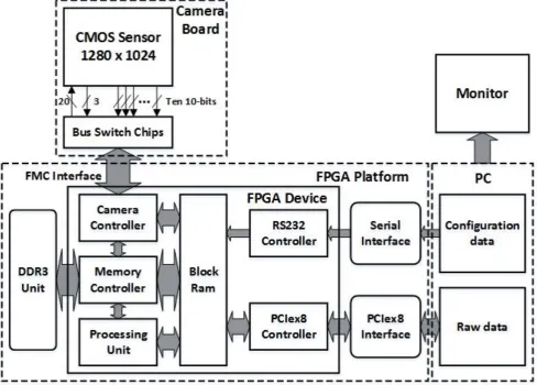
A monochrome CMOS sensor (MT9M413, Micron) having 1280 1024 12 µm 12 µm integrating pixels, 1280 10-bit resolution analogue to digital converters and ten 10-bit-wide digital output ports is driven by an FPGA device (Virtex-6, Xilinx) via a high-speed interface (VITA 57.1 FMC HPC). Due to the large amount of data acquired, a DDR3 SDRAM with capacity of 512 MB is used as internal storage to temporarily store the captured raw data. All controls and processing operations are carried out by the FPGA, and only the processed flow, concentration, speckle contrast and averaged DC images are sent to the PC via a PCIe8 bus.
In operation, a sub-window of 1280 32 pixels is captured and each pixel is sampled at 11.6 kHz. After acquiring the required numbers of samples for FFT operation, the next sub-window is sampled. There is a trade-off between refresh rate and image size as small regions allow high frame rates, while electronic scanning provides high spatial resolution images (up to 1280 1024 pixels if the sub-window is scanned 32 times).
To enable the same photons to be used for comparison of LDI and LSCI we need to simulate the relatively long exposure times required for LSCI using the high frame rate system. For LDI, each sub-frame is sampled at 11.6 kHz with the exposure time of 85 µs. For LSCI, speckle contrast is sensitive to exposure time, and an optimized exposure time is desired for measuring a specific range of velocities, e.g. 5 ms exposure time is optimal for imaging of stimulus-induced changes in cerebral blood flow in rodents [32]. Typically, the optimal exposure time for measuring blood flow is much longer than the one used for the system described here. In order to simulate the longer exposure times associated with LSCI, several short exposure frames are accumulated. It is worth noting that the exposure time simulation is only valid when the inter-frame time (𝛥𝑡) is much smaller than the intensity correlation time [33]. In this system, the inter-frame time is fixed at 1.2 µs which is at least 100 times less than the typical intensity correlation time of moving RBCs (0.1 ms ~ 20 ms). As a result, longer exposure time in LSCI can be simulated by accumulating several short exposure frames in this system.
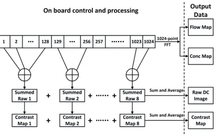
The pipeline structure of the CMOS sensor enables the exposure and the read out to be conducted simultaneously. This means that frame n is exposed as frame n-1 is being read out. Hence, any two adjacent frames can be considered as continuously exposed and thus can be accumulated to simulate a long exposure time. Fig. 2 shows an example where 1024 samples are acquired at an exposure time of 85 µs. In common with most laser Doppler systems flow is calculated by taking the FFT operation, frequency weighting and summing over a frequency range (60 Hz to 5.8 kHz in this case). Concentration is obtained using the same process but without the frequency weighting. In this example the exposure time for LSCI is 10.9 ms and this is achieved by accumulating 128 exposures. To ensure same optical signals to be used for comparison i.e. to use the same number of photons, the contrast maps and DC images are summed a further 8 times. Using this method different exposure times for LSCI can be easily investigated.
3.2.Experimental Setup
A rotating diffuser was adopted to test this system and make the comparison between single exposure LSCI and LDI. The rotating diffuser provides a controlled sample that acts as a flow model for a quantitative comparison. The rotating diffuser (white cardboard) spins behind a static circular glass diffuser, mimicking static tissue overlying moving blood cells. This generates velocity profiles that can be controlled through the motor drive voltage and which change linearly with radial position on the diffuser.
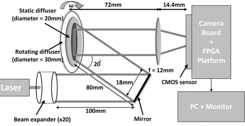
Fig. 3 shows the experimental setup. A green laser (OXXIUS S.A. 532 S-50-COL-PP, = 532 nm, Power = 50 mW) is expanded to a diameter of 18 mm (beam expander, Thorlabs BE20M) and is then reflected onto a static diffuser (diameter 20 mm) with an illumination angle of 20 degrees. A white cardboard disc (diameter 30 mm), which is placed behind the diffuser, spins at a known angular velocity determined by the motor drive voltage. A C-Mount convex lens (Schneider, f = 12 mm) allowing control of aperture size and working distance is placed 72 mm away from the diffuser which forms an image of the diffuser on the CMOS sensor with magnification of 0.2.
The distance between the peak and first local minimum of a speckle is given by [34]
1
.
2
(
1
M
)
f
#
where 𝑀 is the magnification of the imaging system and 𝑓# is the f-number of the lens. In LSCI the distance between fringes is more commonly used [35], [36].#
)
1
(
44
.
2
M
f
speckle
(10)averaged contrast maps were produced due to the small reduction in resolution caused by the processing method (7 7 square). All images were cropped to 160 160 pixels for display. The diffuser was rotated at angular velocities of 0.10, 0.20, 0.27, 0.34, 0.41, 0.54, 0.61, 0.68, 0.75, 0.82, 0.88, 0.95 rad/s. 1024 FFT samples were utilized by LDI processing, and as described in Subsection 3.1 and different numbers of frames were accumulated for LSCI to simulate exposure times of 0.34 ms, 0.69 ms, 1.4 ms, 2.7 ms, 5.4 ms and 22.0 ms.
4.
Experimental Results
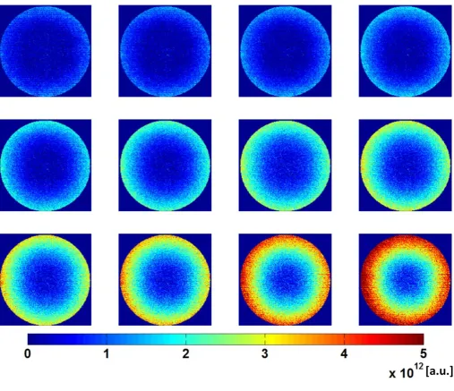
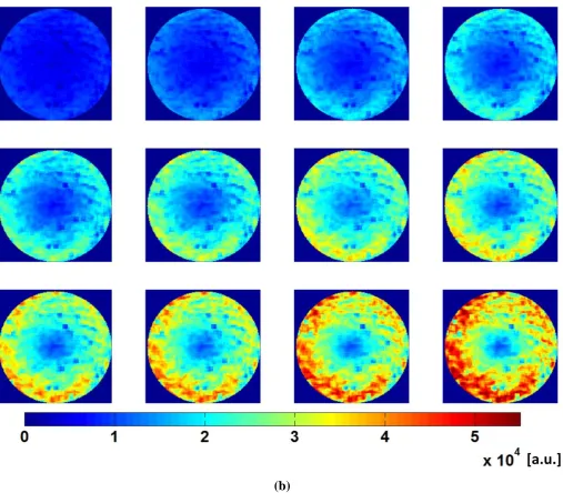
Fig. 4 (a) and (b) show the flow maps of LDI (Eq. (1)) and the velocity distribution maps of LSCI (
1
/
c) for an exposure time of T = 1.4 ms. The rotation angular velocity increases from 0 rad/s to 1 rad/s (left to right and top to bottom) with a fixed increment of 0.034 rad/s, and 31 velocity maps are produced (a selection of 12 images is shown in Fig. 4.).Each method can monitor the increase of speed as the LDI flow values and LSCI flow index values (
1
/
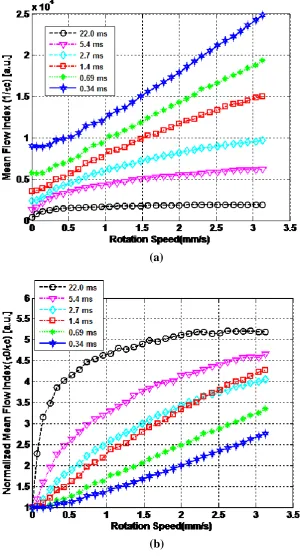
c) rise with both rotation speed and radial position on the disc. It can also be clearly observed that higher values are shown towards the edge of rotating disk as the higher velocity at the edge. The spatial resolution of LSCI is lower than LDI as a 7 7 pixel sub-array is selected to calculate the contrast. Fig. 5 shows the calibrated mean velocity plotted against different disc speeds averaged over all radial positions that have a radius of 3 mm. The mean velocities of LDI and LSCI were calibrated according to Eq. (3) and Eq. (4) respectively by using two known reference velocities of 0.07 mm/s and 3.03 mm/s. Although each curve rises as the speed increases, LDI demonstrates a more linear relationship between the measured and actual velocities.It is well known that LSCI measurement is exposure time dependent. To investigate this in more detail, the experiment is repeated with different equivalent exposure times of 0.34 ms, 0.69 ms, 2.7 ms, 5.4 ms, and 22.0 ms. Fig. 6(a) shows that there is clearly a strong dependence upon exposure time with the measured mean flow index (
1
/
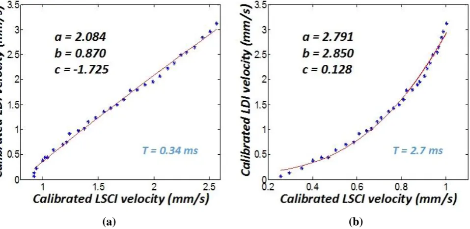
c) being higher for shorter exposure times. For the longer exposure times e.g. T = 22 ms, the speckle is averaged out as velocity increases and so it becomes insensitive to velocity changes. The normalized mean flow index (divided by the static values [38]) is shown in Fig. 6(b) across the range of rotation speeds. Fig. 6(b) shows that longer exposure times (e.g. 22.0 ms and 5.4 ms) have a higher normalized value, and the curves increase rapidly at low speed but reach a limit as motor speed increases. In contrast, shorter exposure times (e.g. 0.34 ms, 0.69 ms) have a flat region at low speed which then rises as the speed increases. The flat region is because the speckle pattern does not have sufficient time to change within a short exposure time. The results clearly show that LSCI is exposure time dependent with a longer exposure time being more sensitive to slow speeds, and shorter exposure times being more suitable to detect changes at higher speeds.Fig. 7 investigates the relationship between velocities calculated using LDI and LSCI using fitting results obtained using Eq.(5) at different exposure times of LSCI, (a) for 0.34 ms and (b) for 2.7 ms. At short exposure times the relationship is close to linear whereas it becomes non-linear at longer exposure times. The linearity indicator, exponent 𝑏, is also plotted against all exposure times in Fig. 7(c).
As can be seen, the exponent, 𝑏, increases with exposure time. If the exposure time is short enough, a value of 𝑏 around 1 can be obtained, which means it is possible to linearly relate LSCI to LDI. However, with longer exposure times (i.e. > 2.7 ms which is typically applied for in vivo measurements) the power function provides a better fit between LSCI and LDI.
5.
Discussion
A high spatial resolution, high frame rate hybrid system has been developed which has a unique pipeline structure that enables the captured frames to be continuously exposed and processed. Different exposure times of LSCI are achieved by accumulating different numbers of adjacent frames equivalently. Based on this structure, the two interchangeable methodologies of imaging blood perfusion, laser Doppler imaging and laser speckle contrast imaging, are integrated on this single device and share the same photons. Consequently, a direct comparison between LDI and LSCI can be achieved.
Well-known characteristics of LDI and LSCI were also verified from the comparison. Due to the differences between the processing methods, LDI has 49 times higher spatial resolution than LSCI. On the other hand, LSCI is faster than LDI by a factor ranging from several times up to a few hundred times depending on the exposure times of LSCI and frequency resolution of LDI (the number of FFT points selected). Laser Doppler imaging has a linear response to speed changes over the whole range of detectable velocities. Laser speckle imaging is exposure time dependent, and the sensitivity and linearity vary as the exposure time changes. With shorter exposure time, the processing is sensitive to higher velocities. However, the sensitivity to the slower speed range is much poorer than that provided by longer exposure times.
is that, as the adopted commercial CMOS sensor is for generic applications, there is no anti-aliasing filter present. Consequently, aliasing occurs when the detected signals has frequencies higher than 5.8 kHz, which affects the linearity of LDI. This could partially be overcome by calibration or alternatively through the use of CMOS sensors with on-chip processing [27], [28]. For LSCI, the summation of multiple short exposures produces a similar signal level to long single exposure but the noise is proportional to sum of the square roots of each exposure time. This will introduce an additional error when applying the spec kle model (Eq. (2)) but it has been demonstrated that in practice this is not a significant effect [39]. There is a source of error that due to the static speckle pattern from the static diffuser which contributes to several “hot” pixels. These contribute to several 7 7 squares with very high contrast value (corresponding to low velocity), which can be observed from the mean velocity maps of LSCI (Fig. 4(b).). The static speckle pattern contributes to unwanted signals but LDI is relatively immune to surface reflections. In LSCI this can be reduced by using cross-polar detection [14].
To overcome the dependence of LSCI on exposure time and static speckle, multi-exposure LSCI (MLSCI) has been introduced [39-41] in which consecutive frames with different exposure times are used to obtain a more accurate blood perfusion value. However MLSCI reduces the frame rate and typically, it is necessary to regulate the light level for specific exposure times to ensure that the pixel intensity is within the dynamic range of the detector. The method described here of simulating different exposure times simultaneously using a high frame rate camera can be used to greatly simplify multi-exposure LSCI by removing the need to adjust light level dynamically [39]. It also increases the frame rate as this will be set by the longest exposure time required for the speckle processing, rather than the sum of all exposure times.
The frame rate of the system is flexible and depends on the spatial resolution and the frequency resolution (number of FFT samples). Table 1 lists the practical frame rates of the processed images with different resolutions and measured samples. They are not the maximum achievable frame rates since the bottleneck of the interface linking the system to the PC decreases the actual frame rate. This means the frame rate can be increased further by developing a faster digital interface.
TABLE1
FRAME RATE OF BLOOD PERFUSION IMAGES (UNIT: FPS)
N o . o f F FT s a mpl es Spatial Resolution*
320320
(314314)
640640
(634634)
12801024
(12741018)
2048 0.286 0.117 0.049
1024 0.593 0.210 0.084
512 1.015 0.344 0.132
256 1.642 0.504 0.182
128 2.283 0.660 0.225
*The number in the bracket indicates the spatial resolution of the LSCI contrast map. As the contrast processing uses 7 7 local pixels, the resolution of blood perfusion images is at the expense of 6 columns and 6 rows.
6.
Conclusion
Two popular optical techniques for blood flow imaging, laser Doppler imaging and laser speckle contrast imaging were compared through imaging a rotating diffuser. For the first time this was achieved using the same detected photons and concurrently applying the different signal processing algorithms. This was enabled by developing a system employing a high frame rate CMOS sensor and a field programmable gate array. As anticipated LDI measurements are linearly related to flow. LSCI is sensitive to static speckle and exposure time although these effects may be reduced by use of multi-exposure laser speckle imaging. The combined measurements demonstrate that the two techniques can be related through a linear relationship at short exposure times and a power law relationship at the longer exposure times typically employed for blood flow imaging.
Acknowledgement
This work was partially supported by an Engineering and Physical Sciences (EPSRC) UK Knowledge Transfer Secondment.
Reference
[1] Hop, M. J., van Baar, M. E., Nieuwenhuis, M. K., Dokter, J., Middelkoop, E., & van der Vlies, C. H., “Determining burn depth: clinical assessment and laser Doppler imaging”, Ned Tijdschr Geneeskd., 156.31 (2012): A4810.
[2] Jayanthy, A. K., Sujatha, N., and Reddy, M.R., (2011), “Laser Speckle Contrast Imaging for Perfusion Monitoring in Burn Tissue Phantoms”, BIOMED, IFMBE Proceedings, 35 (2011): 443-446.
[4] Srienc, A. I., Nelson, Z. L. K., and Newman, E. A., “Imaging retinal blood flow with laser speckle flowmetry”, Front Neuroenergetics, 2 (2010): 128. [5] Forst, T., Weber, M.M., Mitry, M., Schondorf, T., Forst, S., Tanis, M., Pfutzner, A., and Michelson, G.,” Pilot Study for the Evaluation of Morphological
and Functional Changes in Retinal Blood Flow in Patients with Insulin Resistance and/or Type 2 Diabetes Mellitus”, Journal of Diabetes Science and Technology, 6.1. (2012): 163-163.
[6] Humeau, A., Buard, B., Chapeau-Blondeau, F., Rousseau, D., Mahe, G., and Abraham, P., “Multifractal analysis of central (electrocardiography) and peripheral (laser Doppler flowmetry) cardiovascular time series from healthy human subjects”, IOP. Physiol. Meas., 30.7 (2009): 617-629.
[7] Bricq, S., Mahe, G., Rousseau, D., Humeau-Heurtier, A., Chapeau-Blondeau, F., Varela, J.R., and Abraham, P., “Assessing spatial resolution versus sensitivity from laser speckle contrast imaging: application to frequency analysis”, Medical & Biological Engineering & Computing October, 50.10 (2012): 1017 – 1023.
[8] Armitage, G. A., Todd, K.G., Shuaib, A., and Winship, I.R., “Laser speckle contrast imaging of collateral blood flow during acute ischemic stroke”, Journal of Cerebral Blood Flow & Metabolism, 30.8 (2010): 1432-1436.
[9] Li, N., Pelled, G., Gilad, A., Walczak, P., and Thakor, N. V., “An in vivo optical system: control and monitor cortical activity with improved laser speckle contrast imaging and optogenetics”, In Neural Engineering (NER), 2011 5th International IEEE/EMBS Conference on (pp. 76-79), IEEE.
[10] DeFazio, R. A., Zhao, W., Deng, X., Obenaus, A., & Ginsberg, M. D., “Albumin therapy enhances collateral perfusion after laser-induced middle cerebral artery branch occlusion: a laser speckle contrast flow study”, Journal of Cerebral Blood Flow & Metabolism 32.11(2012).
[11] Tchvialeva, L., Dhadwal, G., Lui, H., Kalia, S., Zeng, H., McLean, D. I., and Lee, T.K., “Polarization speckle imaging as a potential technique for in vivo skin cancer detection”, J. Biomed. Opt, 18.6 (2013): 061211-061211.
[12] Hunger, R. E., Torre, R.D., Serov, A., and Hunziker, T., “Assessment of melanocytic skin lesions with a high-definition laser Doppler imaging system”, Skin Research and Technology, 18.2 (2012): 207-211.
[13] Belcaro, G. V., Hoffmann, U., Bollinger, A., and Nicolaides, A.N., “Laser Doppler”, Med-orion Publishing Company, pp. 293, ISBN: 9963-592-53-8. [14] Briers, J. D., “Laser Doppler, speckle and related techniques for blood perfusion mapping and imaging”, Physiol. Meas., 22.4 (2001): R35.
[15] Briers, J. D., “Laser Doppler and time-varying speckle: a reconciliation”, J.Opt. Soc. Am. A, 13.2 (1996): 345-350.
[16] Forrester, K. R., Stewart, C., Tulip, J., Leonard, C., and Bray, R.C., “Comparison of laser speckle and laser Doppler perfusion imaging: measurement in human skin and rabbit articular tissue”, Med. Biol. Eng. Comput., 40.6 (2002): 687-697.
[17] Stewart, C. J., Frank, R., Forrester, K. R., Tulip, J., Lindsay, R., and Bray, R. C., “A comparison of two laser-based methods for determination of burn scar perfusion: laser Doppler versus laser speckle imaging”, Burns, 31.6 (2005): 744-752.
[18] Millet, C., Roustit, M., Blaise, S., and Cracowski, J. L., “Comparison between laser speckle contrast imaging and laser Doppler imaging to assess skin blood flow in humans”, Microvascular Research 82.2 (2011): 147 – 151.
[19] Garry, A. T., Klonizakis, M., Crank, H., Briers, J.D., and Hodges, G.J., “Comparison of laser speckle contrast imaging with laser Doppler for assessing microvascular function”, Microvascular Research, 82.3 (2011): 326 – 332.
[20] Humeau-Heurtier, A., Mahe, G., Durand, S., and Abraham, P., “Skin perfusion evaluation between laser speckle contrast imaging and laser Doppler flowmetry”, Optics Communications, 291 (2013): 483-487.
[21] Binzoni, T., Humeau-Heurtier, A., Abraham, P., & Mahe, G., “Blood perfusion values of laser speckle contrast imaging and laser Doppler flowmetry: is a direct comparison possible?”, Biomedical Engineering, IEEE Transactions on, 60.5 (2013), 1259-1265.
[22] Thompson, O., Bakker, J., Kloeze, C., Hondebrink, E., and Steenbergen, W., “Experimental comparison of perfusion imaging systems using multi-exposure laser speckle, single-exposure laser speckle, and full-field laser Doppler”, Proc. SPIE 8222, Dynamics and Fluctuations in Biomedical Photonics IX, 822204 (February 9, 2012).
[23] Serov, A., Steenbergen, W., and de Mul, FF., “Laser Doppler perfusion imaging with a complementary metal oxide semiconductor image sensor”, Opt. Lett., 27.5 (2002): 300-302.
[24] Serov, A., and Lasser, T., “High-speed laser Doppler perfusion imaging using an integrating CMOS image sensor”, Opt. Express, 13.17 (2005): 6416-6428. [25] Draijer, M., Hondebrink, E., Leeuwen, T.v., and Steenbergen, W., “Twente Optical Perfusion Camera: system overview and performance for video rate
laser Doppler perfusion imaging”, Optics Express, 17.5 (2009): 3211-3225.
[26] Leutenegger, M., Martin-Williams, E., Harbi, P., Thacher, T., Raffoul, W., André, M., Lopez, A., Lasser, P., and Lasser, T., “Real-time full field laser Doppler imaging”, Biomed Opt Express, 2.6 (2011): 1470–1477.
[27] He, D., Nguyen, H.C., Hayes-Gill, B.R., Zhu, Y., Crowe, J.A., Clough, G.F., Gill, C.A., and Morgan, S.P., “64×64 pixel smart sensor array for laser Doppler blood flow imaging”, Opt Lett., 37.15 (2012): 3060-3062.
[28] He, D., Nguyen, H.C., Hayes-Gill, B.R., Zhu, Y., Crowe, J.A., Clough, G.F., Gill, C.A., and Morgan, S.P., “Laser Doppler Blood Flow Imaging Using a CMOS Imaging Sensor with On-Chip Signal Processing,” Sensors, 13(9), 12632-12647.
[29] Serov, A., and Lasser, T., “Combined laser Doppler and laser speckle imaging for real-time blood flow measurements”, Proc. of SPIE, 6094 (2006): 06-06. [30] Bonner, R., and Nossal, R., “Model for laser Doppler measurements of blood flow in tissue”, OSA, Appl. Opt., 12.20 (1981): 2097-2107.
[31] Draijer, M., Hondebrink, E., van Leeuwen, T., & Steenbergen, W., “Review of laser speckle contrast techniques for visualizing tissue perfusion”, Lasers in medical science, 24(4), 639-651.
[32] Yuan, S., Devor, A., Boas, D., and Dunn, A., “Determination of optimal exposure time for imaging of blood flow changes with laser speckle contrast imaging”, Appl Opt., 44.10 (2005): 1823–1830.
[33] Zakharov, P., Völker, A. C., Wyss, M. T., Haiss, F., Calcinaghi, N., Zunzunegui, C., Buck, A., Scheffold, F., and Weber, B., “Dynamic laser speckle imaging of cerebral blood flow”, Opt. Express, 17.16 (2009): 13904-13917.
[34] Ennos, A. E., "Speckle interferometry.", In Laser speckle and related phenomena, Springer Berlin Heidelberg (1975): 203-253.
[35] Boas, D.A. and Dunn, A.K., “Laser speckle contrast imaging in biomedical optics”, Journal of biomedical optics, 15.1 (2010): 011109-011109. [36] Cloud, G., “Optical methods in experimental mechanics”, Experimental Techniques, 34.6 (2010): 11-14.
[37] Kirkpatrick, S. J., Duncan, D.D., and Wells-Gray, E.M., “Detrimental effects of speckle-pixel size matching in laser speckle contrast imaging”, Optics Letters, 33.24 (2008): 2886–2888.
[38] Cheng, H., and Duong, T., “Simplified laser-speckle-imaging analysis method and its application to retinal blood flow imaging”, Opt Lett, 32.15 (2007): 2188–2190.
[39] Sun, S, Hayes-Gill, B.R., He, D., Zhu, Y. and Morgan, S.P., “Multi-exposure laser speckle contrast imaging using a high frame rate CMOS sensor with a field programmable gate array”, Optics Letters 40.20 (2015): 4587-4590.
[40] Parthasarathy, A. B., Tom, W. J., Gopal, A., Zhang, X., and Dunn, A. K., “Robust flow measurement with multi-exposure speckle imaging”, Opt. Express, 16.3 (2008): 1975-1989.
Biographies
Shen Sun received his B.Eng degree in Electronic and Information Engineering from BeiHang University, China, in 2008 and MSc and PhD degrees in Electronic Engineering from the University of Nottingham in 2009 and 2013 respectively. This was followed by a two year period as a research fellow at the University of Nottingham working on biomedical optics. His research focuses on full-field laser Doppler and laser speckle contrast blood flow imaging systems in the application and development of medical devices and healthcare instruments.
Barrie Hayes-Gill is Professor of Electronic Systems & Medical Devices at The University of Nottingham where he holds BEng & PhD degrees. He has worked as a Senior Engineer at Texas Instruments, AEI and Marconi Electronic Devices and is a Fellow of the Institution of Engineering and Technology (FIET). His research interests are in opto-electronics and integrated circuit design applied to biomedical devices often returning to industry to maintain industrial relevance. He has published over 250 papers, holds 13 patents and is a director of 2 University spin out companies.
Diwei He received the B.Eng. degree from the Southeast University, China, in 2002 and the MRes and PhD from the University of Nottingham, UK, in 2004 and 2008 respectively, all in electrical and electronic engineering. His doctoral research focused on the design of a full-field laser Doppler blood flow imaging sensor. He then worked at the University of Nottingham as a research fellow with primary research interests in designing analogue and mixed-signal electronic systems for physiological
measurements. He joined Monica Healthcare Ltd in 2014 to develop the next generation of wireless fetal ECG monitoring systems.
Nam T. Huynhreceived his B.Eng in electronic engineering from Hochiminh city University of Technology, Vietnam, in 2003 and the MSc and PhD from the University of Nottingham, UK in 2005 and 2009, respectively. His doctoral thesis specialised in novel optical scattering techniques for particle sizing. He then spent 3 years as a research fellow at Nottingham working on various tissue imaging techniques. Since 2012, he has been working at the University College London Photoacoustic imaging group. His primary interests are acousto-optic s, photoacoustics, and light-tissue interaction
(a)
Fig. 4 (a) LDI flow maps of LDI and (b) LSCI velocity distribution maps simultaneously obtained at rotation speeds of 0.10, 0.20, 0.27, 0.34, 0.41, 0.54, 0.61, 0.68, 0.75, 0.82, 0.88, 0.95 rad/s (top left to bottom right). The image area is 9.6 mm 9.6 mm and the scale ranges are from 0 to 5 × 10¹² for LDI, from 0 to
[image:13.595.42.550.68.505.2](b)
Fig. 4 (a) LDI flow maps of LDI and (b) LSCI velocity distribution maps simultaneously obtained at rotation speeds of 0.10, 0.20, 0.27, 0.34, 0.41, 0.54, 0.61, 0.68, 0.75, 0.82, 0.88, 0.95 rad/s (top left to bottom right). The image area is 9.6 mm 9.6 mm and the scale ranges are from 0 to 5 × 10¹² for LDI, from 0 to
[image:14.595.43.551.67.511.2](a)
[image:16.595.50.353.77.634.2](b)
(a) (b)
[image:17.595.54.533.84.317.2]Figure Captions
Fig. 1 Schematic of the system showing the main imaging, processing, control and storage units. The CMOS sensor interfaces to the FPGA via the custom-made FMC socket mounted on an 8-layer PCB board (camera board). Various controllers including camera controller, memory controller, RS232 controller and PCIe8 controller are developed in the FPGA along with the processing unit (processing algorithms) for achieving the functionality. The PC-generated configuration data is sent to the system via the serial interface (RS232). The processed data (blood flow images, blood concentration images, contrast maps and DC images) are transmitted to the PC for further processing and display through the PCIe8 bus. This figure is a reproduced material which was originally produced for [36].
Fig. 2 Digital structure to enable the same photons to be processed for both LDI and LSCI (1024 samples for LDI, equivalent 10.9 ms exposure time for LSCI). Every 128 frames of the total 1024 frames are accumulated to simulate a longer exposure time of 10.9 ms. To use all the data of LDI for LSCI processing, the contrast map obtained by processing the speckle pattern image with equivalent 10.9 ms exposure time is averaged a further 8 times.
Fig. 3 Rotating diffuser experimental setup. A white cardboard disc spinning behind a static circular glass diffuser simulates blood flow in tissue. = 532 nm, laser light is expanded and illuminates the sample (via a mirror). The rotating diffuser is imaged onto the CMOS sensor through a convex lens (f = 12 mm). This figure is a reproduced material which was originally produced for [36].
Fig. 4 (a) LDI flow maps of LDI and (b) LSCI velocity distribution maps simultaneously obtained at rotation speeds of 0.10, 0.20, 0.27, 0.34, 0.41, 0.54, 0.61, 0.68, 0.75, 0.82, 0.88, 0.95 rad/s (top left to bottom right). The image area is 9.6 mm 9.6 mm and the scale ranges are from 0 to 5 × 10¹² for LDI, from 0 to
5.5 × 10⁴ for LSCI.
Fig. 5 Calibrated mean velocity at a fixed radius (3 mm) for different motor drive speeds. The exposure time of LSCI is 1.4 ms. The error bar shows the standard deviation of the calibrated mean velocity values of all pixels in the same radial position.
Fig. 6. Effect of exposure time on mean speckle variance values (a) absolute (b) normalized relative to value at 0mm/s speed. Longer exposure times are more sensitive to low speed, while the speckle pattern is fully blurred when the speed is relatively high. In contrast, shorter exposure times cover a wider range of detectable velocity however it is insensitive to velocity changes at low speed.