The linear inverse problem in energy beam processing with an
application to abrasive waterjet machining
A. Bilbao Guillerna
a, D. Axinte
a,n, J. Billingham
b aMachining and Condition Monitoring Group, Faculty of Engineering, The University of Nottingham University Park, NG7 2RD, UK bSchool of Mathematical Sciences, The University of Nottingham University Park, NG7 2RD, UK
a r t i c l e i n f o
Article history:
Received 17 April 2015 Received in revised form 2 September 2015 Accepted 2 September 2015 Available online 10 September 2015
Keywords:
Inverse problem Controlled depth etching Energy beam
Abrasive waterjet machining
a b s t r a c t
The linear inverse problem for energy beam processing, in which a desired etched profile is known and a trajectory of the beam that will create it must be found, is studied in this paper. As an example, abrasive waterjet machining (AWJM) is considered here supported by extensive experimental investigations. The behaviour of this process can be described using a linear model when the angle between the jet and the surface is approximately constant during the process, as occurs for shallow etched profiles. The inverse problem is usually solved by simply controlling dwell time in proportion to the required depth of milling, without considering whether the target surface can actually be etched. To address this, a Fourier analysis Is used to show that high frequency components in the target surface cannot be etched due to the geometry of the jet and the dynamics of the machine. In this paper, this frequency domain analysis is used to improve the choice of the target profile in such a way that it can be etched. The dynamics of the machine also have a large influence on the actual movement of the jet. It is very difficult to describe this effect because the controller of the machine is usually unknown. A simple approximation is used for the choice of the slope of a step profile. The tracking error between the desired trajectory and the real one is reduced and the etched profile is improved. Several experimental tests are presented to show the use-fulness of this approach. Finally, the limitations of the linear model are studied.
&2015 The Authors. Published by Elsevier Ltd. This is an open access article under the CC BY-NC-ND license (http://creativecommons.org/licenses/by-nc-nd/4.0/).
1. Introduction
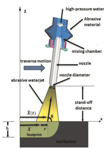
Abrasive Waterjet Machining (AWJ) machining is a fast-grow-ing non-conventional technology capable of processfast-grow-ing any ma-terial regardless of its properties. Modern AWJ machining systems make use of high-pressure water jets (up to 90 000 psi¼620 MPa) forced through a tiny orifice (0.1–0.3 mm) that enables the en-trainment and acceleration of abrasive particles (e.g. garnet, Al2O3) to high velocities (200–800 m/s). When the resulting three-phase jet plume (water, abrasives and air, [1]) impacts a target surface, it removes material by abrasive erosion (i.e. erosion by solid particle impingement)[2–4].
The inverse problem consists of defining the control para-meters, in particular the 3D beam path (position and orientation of the beam as a function of time), to create a prescribed freeform surface. This inverse problem is well understood for conventional machining (e.g. turning, grinding, drilling), because the cutting tool geometry is well defined and the material removal is atime independent process. In contrast, energy beam (EB) machining is achieved through the local interaction of an energy beam of
particular characteristics (e.g. energy distribution), which leads to a time-dependent removal rate. Furthermore, EB machining is a time-dependent process in which not only does the etched surface vary with the dwell time, but also any acceleration or deceleration of the machine/beam delivery system when performing raster paths will influence the actual geometry of the surface generated. This makes the process inherently nonlinear, and dependent upon good mathematical models, which then have to be inverted to produce a suitable beam path, i.e. solving the inverse problem.
Some research in addressing the direct problem, i.e. given a model for the footprint and the beam path, to determine the generated surface, has been reported. Some of the most common methods are based on statistical approaches[5], finite element methods[6–8]or artificial intelligence methods[9]. Finite element methods have also been used to model overlapped footprints[10]. However, there are some important drawbacks to these three methods: statistical methods are only valid if the operating para-meters are near the ones used for the modelling;finite element approaches are computationally expensive and simplifying hy-potheses are needed; artificial intelligence approaches requires significant sets of data for training and give little insight into the details of the physics that affect the process.
There is another set of more thorough approaches for Contents lists available atScienceDirect
journal homepage:www.elsevier.com/locate/ijmactool
International Journal of Machine Tools & Manufacture
http://dx.doi.org/10.1016/j.ijmachtools.2015.09.006
predicting footprint profiles based on analytical/geometric mod-elling. One of thefirst studies details a model of the footprints of stationary air powder-blaster jets [11]. The advantage of such models is their relationship to the physical process of material removal and their ability to predict the jet footprint whenever the initial conditions are known[12]. This approach has been mainly used for the prediction of single trenches when the jet impinge-ment angle is
π
/2 rad and the path used is straight[13]. Recently, some studies have been published that consider free-moving tra-jectories of the jet[14]and the effect of the overlapping of raster paths[15].In contrast, the inverse problem in EB controlled-depth ma-chining, the more technically important and yet academically challenging problem, has not been studied in detail. The most common strategy is simply to vary the dwell time of the beam on each pixel of the target surface [16]. This is simply the leading order approximation to the necessary strategy when the radius of the beam is small compared to the size of the feature that is being etched. There has been some work on the inverse problem for other time-dependent processes: electro-chemical machining[17], where the tool/electrode works in tangential mode to envelope the required surface and is more similar to the movement of a cam than to the energy beam inverse problem; electro-discharge ma-chining[18]where the electrode, with wear pattern measured at time intervals, copies the geometry of the final surface, so a mathematical solution to the inverse problem is not required.
In this paper a new approach to the inverse problem for EB processes, with an emphasis on abrasive Waterjet Machining (AWJM) is presented. Most of the previous solutions just consist of varying the dwell time in proportion to the required depth of milling to achieve the desired surface. However, they do not consider whether a solution to the inverse problem actually exists. In other words, the target surface is usually defined without checking whether the process can etch that particular surface. We will show below that some frequency components, usually high frequency ones, cannot be etched due to the geometry of the jet. A Fourier analysis can be used tofind a solution to this problem. This approach gives information about what kind of surfaces can be etched by checking the influence of each frequency on the etched surface. Moreover, an exact solution to the problem can be cal-culated. The dynamics of the machine also have a large influence on the actual trajectory of the energy beam. Developing an un-derstanding of and a model for these dynamics is difficult, because most of the control parameters of the machine are not accessible to the user. However, for some particular profiles the machine dynamics can be compensated. In[19], the slope of a ramp on the target surface is calculated using the maximum value of the jerk that the AWJM can achieve. This seems to be thefirst approach to consider the dynamics of the machine tool when precise surfaces are required in EB machining and further analysis is needed for more complicated surfaces where the behaviour of the machine changes during the trajectory. However, this approach is good enough to select the appropriate value of the slope of a ramp. The tracking error between the desired trajectory and the target one is reduced and the quality of the etched surface is improved.
1.1. Scope of the paper
The inverse problem is studied for a general EB process, with particular emphasis on its application to AWJ machining. To achieve this scope the following aspects have been investigated:
1. For shallow surfaces a linear model describes the process well, and a frequency domain analysis can be performed to obtain the solution of the inverse problem. This approach gives informa-tion about what kind of surfaces can be etched.
2. The machine dynamics are compensated when a step is in-cluded in the target surface; the maximum value of the jerk is measured and used to decide the slope of the ramp.
3. Experimental results indicate when a linear model is valid and when a nonlinear model is needed. Different values of the depths for the target profile are considered and the influence of overlapping between two consecutive passes of the energy beam is studied.
2. Generic model of an energy beam process
A generic partial differential equation model for an energy beam process is
x a p
Z
t E0 , , ,t Z Z; , t , 1
∂
∂ = − ( ∇ ( )) ( )
subject to Z(x, 0) =Z0( )x .In this model, E0is the etching rate function, which characterises the rate of removal of material,tis time, with0≤t≤T, x=(x y, )is spatial position, z=Z(x,t)is the evolving position of the surface in a Cartesian coordinate system,
x y z, ,
( ). In addition, a is a vector of constant parameters that characterize the model andp(t) is a vector of control parameters. The appearance of Z and ∇Z in E0indicates that, in general, the slope of the evolving surface and its distance from the nozzle af-fect the rate at which material is removed. In the forward problem, thefinal surface, Z(x,T), is determined by the choice of control parameters,p(t). In the inverse problem, the objective is tofindp
(t) given a specified target surface, Z(x,T).
In this paper, it is assumed that the initial surface is flat (Z0( )=x 0) and the linearized problem is studied. In the context of AWJM (Fig.1), upon which this paper focuses, this means that the feed speed is assumed to be sufficiently high that nonlinear effects due to the evolving slope of the surface and its distance from the nozzle can be neglected, an assumption that can be tested ex-perimentally. In this case, (1) can be written as the linear equation.
x a p
Z
t E0 , ,0, 0; ,t t . 2
∂
[image:2.595.343.526.474.735.2]∂ = − ( ( )) ( )
In order to make some analytical progress and easily compare theory to experiment, we will further restrict our attention to the case where the axis of the AWJ plume remains perpendicular to the plane,z 0,= of the unetched surface, so that
Z
t E r, 3
∂
∂ = − ( ) ( )
wherer= x X− ( )t is the distance to the centre of the beam,X( )t , projected ontoz=0, which provides the only control parameters, and E r( )is the etching rate function.
As described in Kong et al. (2012) E r( ), can be calibrated ex-perimentally by using a jet with high feed speed to generate a straight, shallow trench, from which E r( )can be calculated using
⎡ ⎣ ⎢ ⎢ ⎢ ⎤ ⎦ ⎥ ⎥ ⎥
E r s Z s Z r
s r
ds Z r r 1 1 . 4 r
f f f
1
2 23 2
2
(
)
∫
(
)
π ( ) = ( ) − ( ) − − ( ) − ( )HereZ yf( )is the measured profile across the trench and distance is
measured in units of beam radius.
3. Linear inverse problem
In the inverse problem the objective is tofind the appropriate values of the control parameters, in this caseX( )t, to obtain afinal surface close to a given target surface. For a nonlinear model of the form given by (1), this is a complex optimization problem that requires significant computational resources and will be the sub-ject of a future paper. By studying the linearized inverse problem, using Eq. (3), significant insight can be gained into some funda-mental limitations on the family of surfaces that can be etched using a beam with a given footprint, E r( ).It also gives a simple framework within which to study the influence of the dynamics of the machine, which experimental tests show to be very significant. The experimental tests discussed inSection 4are all for straight paths etched by a jet with a variable feed speed, which results in straight trenches of variable depth. The centreline of these tren-ches can be treated as the outcome of a one-dimensional etching process. The centreline of these trenches can be treated as the outcome of a one-dimensional etching process. We therefore consider (3) in 1D, so that
Z
t E x X t , 5
∂
∂ = − ( − ( )) ( )
where x is position along the trench, X t( )is the position of the centre of the jet andEis the etching rate function, assumed to be an even function of its argument, obtained using the experimental calibration procedure described above. Thefinal etched surface is
Z x T, E x X t dt.
6 T 0
∫
( ) = − ( − ( )) ( )If we also assume that X t( )is strictly increasing (the jet never retraces its path),1we can write (6) as
Z x T, E x X x D x dx,
7 L L
(
)
∫
( )
( ) = − − ‵ ( ‵) ‵ ( ) −where D x dX
dt 1
( ) ≡ ( )− is the dwell time as a function of position along the path, which runs from x= −Lto x=L. Then, by the convolution theorem,
Zn= −2LE Dn n, ( )8
where
E
L E x e dx
1
2 , 9
n
L L
in x L/
∫
= ( ) ( ) π − −is thenth Fourier component of E x( )and similarly for Zn and
Dn.2
Since En can be calculated from the calibrated etching rate
function, E x( ), as can Znfrom a given target trench depth profile,
Z x T( , ), in principle Dn, and hence the required dwell time profile,
D x( ), can be calculated. However, if En=0 for somen, then that mode has no effect on the etched surface. Moreover, if someEnis
small but nonzero (as is typical for high order modes of the Fourier transform of a function withfinite support) it will lead to a cor-respondingly large value ofDn. It can be concluded that, not only is
there a fundamental restriction on the frequency content of the
final target surface that comes from the frequency content of the etching rate function, but also that, if a given frequency does exist inE x( )but is small, it induces a correspondingly large component in the dwell time,D x( ), and hence in the beam path,X t( ), that may not be realizable in practice due to the dynamics of the AWJ ma-chine, which is discussed below.
4. Compensation of the dynamics of the machine
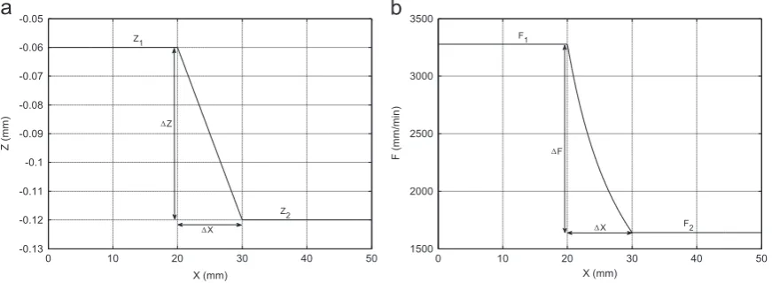
The dynamics of the machine have a big influence on the possible movement of the jet. Although the trajectory of the jet is usually implemented as a CNC file, the controller used by the machine to generate the actual trajectory is usually unknown and the identification of a model valid under any conditions is not an easy task. For example, if a step is defined as in Fig.2(a), where the slope is determined by Z1, Z2 and
Δ
X, then the required feedspeed, calculated using the linear model (3), is shown in Fig.2(b). In this paper two different approaches are used to compensate for the dynamics of the machine when a step like this is implemented in the required trajectory.
4.1. Frequency analysis approach
For a particular step the jet trajectory is calculated and im-plemented in the machine, and then the actual trajectory is measured. The input and measured trajectories are then compared in the frequency domain. A Frequency Response Function (FRF) can be calculated from those signals. For any other step the tra-jectory can be compensated by multiplying by the inverse of the FRF in the frequency domain. From (8),
Zn= −2LE D Hn n n, (10)
whereHnis the FRF calculated as
H X X , 11 n n measured n input = ¯ ¯ ( )
whereXn measured
̅ and Xn
input
̅ are the measured and input trajectories of the beam in the frequency domain. Similar conclusions as in Section 3can be reached in this case with the inclusion of this FRF. If the value ofHn is zero for a particular mode, that frequency cannot appear on the etched surface since it is filtered by the dynamics of the machine. The main advantage of this method is that one can know the range of frequencies that can be included in
1This assumption is not restrictive as a path that reverses its direction can be
replaced with an equivalent unidirectional path within the context of a linear theory.
2
the target surface. However, although this is a convenient frame-work within which to understand how the dynamics of the ma-chine affect the range of surfaces that can be etched, these dy-namics are unavoidably nonlinear. In the experimental tests we therefore used a different approach to compensate the machine dynamics.
4.2. Maximum gradient approach
In this method different values of
Δ
x are considered for a particular step (Fig.2) with constant values forZ1andZ2. For eachvalue of
Δ
xthe response is measured and the value of the gradient of the feed speed,F(x), is calculated in the middle of the step.3For small values of the slope the machine is able to achieve the desired gradient. However, when the gradient is too large it cannot be obtained.In order to compensate for the dynamics the following steps are taken:
1. Define the desired value of the slope (s) for the step in the profile and calculate the gradient ofF(x) in the middle of the step using
s= −KFm−2G F(m) (12)
where Fm=( +F1 F2)/2 is the mean value of the feed speed and G F(m)is the value of the gradient in the middle of the step.F1and F2are the values of the feed speed needed to obtain the target depths,Z1 and Z2.Kis a constant parameter obtained for
ex-perimental data.
2. Use the measured data to calculate the value of
Δ
xthat gives the desired value of the gradient obtained in the previous step. 3. Compensate the look-ahead option of the machine by changing the position of the step. The controller of the machine calculates the trajectory by considering the next points in the commanded input. For this reason the jet starts accelerating or decelerating in a different position. This value is unknown, but it can be compensated if the position of the step is moved.4. Use round corners to avoid the high frequency components that are identified as being impossible to etch using the theoretical results given above.
5. Generate the new target profile with those values and calculate the input trajectory using (8). Since the gradient depends on the sign of
Δ
F¼F2–F1, the etching is always done in one direction(no raster paths)
The proposed method can be summarized as the following steps:
1. First, an experimental shallow trench Is generated to calibrate the linear model described in Eq. (3). the etching rate function,E (r), Is calculated using Eq. (4)
2. The small frequency components in the etching rate function are avoided in the target surface. in particular, High frequencies are not included in the target surface.
3. The trajectory of the beam Is obtained from the inverse of the Fourier transform of the dwell time,Dn, calculated using Eq. (8).
4. Finally, the dynamics of the machine are compensated using the method described inSection 4.
5. Experimental tests
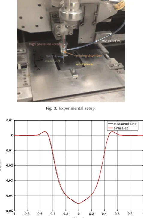
The experimental data for model validation has been generated with a Microwaterjet 3-axis F4 type machine developed by Wa-terjet AG4(Fig.3). Several cutting heads, with a diameter of the mixing nozzle from 0.2 to 0.8 mm, can be mounted in the system. The diameter of the water orifice varies from 0.08 to 0.24 mm. The machine is empowered by a KMT streamline SL-V100D ultra-high pressure pump, capable of delivering a pressure range from 700 to 4000 bar. The apparatus has been designed for high accuracy cutting applications, with a cutting accuracy of 0.01 mm and a positioning accuracy of 0.003 mm, and its maximum traverse speed is 4000 mm/s. The abrasive particles used for this study are BARTON HPX 220. The following constant parameters are con-sidered:P¼138 MPa,ma¼0.03 kg/min, SOD (stand-off distance)¼ 3 mm. The diameters of the mixing and water nozzles are 0.5 mm and 0.18 mm, respectively. The material of the workpiece is Ti6Al4V alloy extensively used for the manufacture of aerospace and medical components.
5.1. Model calibration
First the calibration of the etching rate function has to be performed. In the theory, only one trench is necessary for cali-bration purposes. However, in practice the measured profile varies due to the fluctuations of the pump pressure and the process noise. In order to avoid this limitation several trenches are gen-erated using the same conditions and an experimental profile is measured from each set of data. Then the average of the different
0 10 20 30 40 50
-0.13 -0.12 -0.11 -0.1 -0.09 -0.08 -0.07 -0.06 -0.05
X (mm)
Z (mm)
X
Z2 Z1
Z
0 10 20 30 40 50
1500 2000 2500 3000 3500
X (mm)
F (mm/
mi
n)
F2 F1
F
X
Δ Δ
Δ
[image:4.595.86.522.59.219.2]Δ
Fig. 2.Definition of a step in the target surface (a) and the calculated feed speed of the machine (b).
3
Note that the spatial gradient of the feed speed,F(x), is the acceleration
di-vided by the feed speed. 4
profiles is calculated. Each trench is generated by moving the jet at 3000 mm/min in thex-direction and the average of the profile in they-direction is calculated. In Fig. 4 the average profile is dis-played. Then using (4) the etching rate function can be calculated (Fig. 5). Once the etching rate function is known the process is simulated using (3) and a simulated profile is obtained (Fig.4).
Eq. (4) provides a set of points for the etching rate function. For simulation purposes these points are fitted to an equation. The summation of different sinusoidal functions has been found as the
equation with the bestfitting. The etching rate function in Fig.4 can befitted to
E r a sin b r c 13
k 1 k k k 8
(
)
∑
( )= + ( )
=
with a1¼0.1053; b1¼5.916; c1¼0.798; a2¼0.05573; b2¼11.8;
c2¼1.609; a3¼0.003392; b3¼33.39; c3¼2.911; a4¼0.003818;
b4¼24.07; c4¼3.201; a5¼0.00117; b5¼50.84; c5¼1.917;
a6¼0.001062; b6¼60.79; c6¼2.325; a7¼0.0006665; b7¼71.68;
c7¼2.633;a8¼0.0003799;b8¼83.96;c8¼2.788.
5.2. Frequency domain analysis
In order to show how the frequency domain analysis is used to select the target surface, the profile described in Fig. 6 is con-sidered.Tdescribes the period of the trapezoidal wave and
τ
[image:5.595.40.279.59.423.2]de-fines the length of the ramp. Small values of
τ
lead to larger values of the slope and higher frequency components. In Fig. 7a fre-quency analysis is done for three different values ofτ
.τ
¼0.25 mm (red line) leads to larger values of the high frequency modes. These modes are attenuated forτ
¼1 mm. The Fourier transform of the etching rate function calculated in the previous section is also displayed (dotted black line). The component of the mode of the etching rate function atf¼3 mm1is almost zero. This means that the inclusion of this mode in the target surface would lead to a large value of that mode in the trajectory of the beam. Obviously this is not a good idea and any frequency larger than 3 mm1Fig. 3.Experimental setup.
-1 -0.8 -0.6 -0.4 -0.2 0 0.2 0.4 0.6 0.8 1 -0.05
-0.04 -0.03 -0.02 -0.01 0 0.01
Y (mm)
Z (
m
m)
measured data simulated
Fig. 4.Average profile used for the calibration and simulated one after calibration.
0 0.05 0.1 0.15 0.2 0.25 0.3 0.35 0.4 -0.02
0 0.02 0.04 0.06 0.08 0.1 0.12 0.14
r (mm)
E
[image:5.595.305.551.59.242.2](r)
Fig. 5.Etching rate function, E(r).
0 2 4 6 8 10 12 14
-0.22 -0.2 -0.18 -0.16 -0.14 -0.12 -0.1 -0.08
X (mm) Zr
(mm)
T
τ
Fig. 6.Target surface.
0 1 2 3 4 5 6 7 8 9 10
0 0.5 1 1.5 2 2.5 3 3.5 4 4.5
5x 10
-3
Frequency(x-1)
|Zr|
T = 10 mm
= 1 mm =0.5 mm = 0.25 mm E
[image:5.595.36.282.453.639.2]τ τ τ
[image:5.595.307.549.546.730.2]should be avoided in the trajectory. In particular, target surfaces with
τ
¼1 mm (blue line in Fig.7) andτ
¼0.5 mm (black line in Fig. 7) have a nonzero component atf¼3 mm1. The solution of theinverse problem for these two profiles would lead to large com-ponents around that frequency and undesirable oscillations of the jet.
The target surface is selected in such a way that all the fre-quency components can be etched by the etching rate function. First
τ
is selected in such a way that thefirst minimum is atf¼3 mm1, which happens when
τ
is 0.4 mm (blue line in Fig.8).Moreover, round corners can also be used tofilter the high fre-quencies while the value of the slope of the ramp is kept constant (green line). Finally, the inverse Fourier transform is used to obtain the target profile in the spatial domain,Zr(x).
5.3. Compensating the dynamics of the machine
In order to show how the dynamics of the machine are com-pensated, a particular step described as in Fig.2 is considered, withZ1 ¼0.06 mm and Z2¼0.12 mm. These depths are obtained
with feed speeds F1¼3280 mm/min and F2¼1640 mm/min,
re-spectively. Fig.9shows the measured value of the gradient of the feed speed in the middle of the step as a function of
Δ
X. The ex-periment is performed for both accelerating (red line) and decel-erating cases (blue). Positive (xþ) and negative (x) movements inx-axis of the machine are considered as well. The results showthat there is no difference between the positive (solid line) and the negative (dotted line) axis for the same step. However, the value of the gradient achieved is higher when the machine is decelerating. This is an important aspect to be taken into account since most surfaces are etched using raster paths.
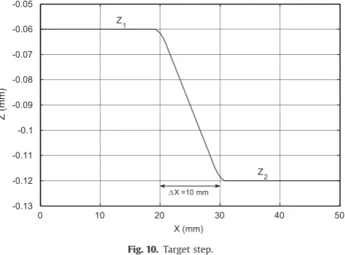
Fig. 10 shows a target surface with Z1¼ 0.06 mm, Z2 ¼ 0.12 mm and
Δ
X¼10 mm. The desired value of the slope at the middle of the step is obtained when the gradient of the speed is 184.5 min1. Now from the results in Fig.8that particular valueof the gradient is achieved when
Δ
x¼7.5 mm. Moreover, the look-ahead option is compensated by delaying the step 4 mm. Fig.11 shows the correction of the trajectory. The red line is the com-pensated trajectory used to generate the input CNC and the black line is the actual measured trajectory of the beam. One can see that the error between the desired trajectory (blue) and the actual trajectory (black) is reduced, while the desired slope in the middle of the step is achieved.5.4. AWJ milling tests for the linear inverse problem
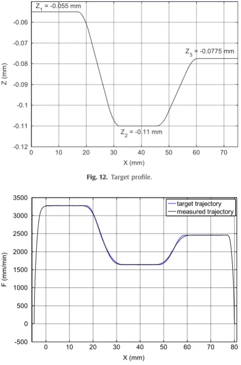
The target profile is displayed in Fig.12. Three different values of the depths are considered. The profile is selected by analysing its Fourier transform and checking that all the frequency compo-nents can be included. Then the dynamics of the machine are compensated using the technique described above. In Fig. 13a comparison between the measured trajectory after the compen-sation and the target one is displayed.
The trajectory is implemented in a milling process and the
0 1 2 3 4 5 6 7 8 9 10
0 0.5 1 1.5 2 2.5 3 3.5 4 4.5
5x 10
-3
Frequency(x-1)
|Zr|
T = 10 mm E
= 0.4 mm (trapezoidal) =0.4 mm (round corner)
[image:6.595.47.292.57.256.2]τ τ
Fig. 8. Final target surface.
0 5 10 15 20
200 400 600 800 1000 1200 1400
X (mm)
max (gradient)
F
1 ---> F2 (x+)
F1 ---> F2 (x-) F2 ---> F1 (x+) F2 ---> F1 (x-)
[image:6.595.317.560.59.238.2]Δ
Fig. 9. Maximum gradient calculated in the middle of the step.
0 10 20 30 40 50
-0.13 -0.12 -0.11 -0.1 -0.09 -0.08 -0.07 -0.06 -0.05
X (mm)
Z (mm)
X =10 mm Z1
Z2
Fig. 10.Target step.
0 5 10 15 20 25 30 35 40 45
1600 1800 2000 2200 2400 2600 2800 3000 3200 3400
X (mm)
F (mm/
mi
n
)
[image:6.595.319.560.559.730.2]measured trajectory target trajectory input trajectory (CNC file)
[image:6.595.46.289.562.730.2]profile is measured. Fig.14compares the measured profile (blue) and the desired one (black). The tracking error is almost zero for two of the target depths, while there is a small error in the deepest one. Nonlinear effects have more influence at larger depths, since the angle between the jet and the etched surface is larger. More-over, the measured values of the slopes of both ramps are also close to the target values.
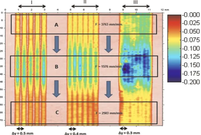
Finally, in order to investigate the limitations of the assumption of linearity, the same trajectory is repeated and the trenches
allowed to overlap. Overlapping describes the distance between two consecutive passes in they-direction (
Δ
Y). Three different overlapping values are considered:Δ
Y¼0.5 mm (0%),Δ
Y¼0.4 mm (20%) andΔ
Y¼0.3 mm (40%), represented by Sec-tions I, II and III, respectively in Fig.15. Figs.16–18 show the average profiles in they-direction for the part of the trajectory with constant speed (and hence constant depth). Sections A, B and C correspond to the constant feed speed parts equal to 3763 mm/ min (blue lines), 2503 mm/min (black lines) and 1576 mm/min (red lines), respectively. In Figs.16–19, the experimental data is displayed with solid lines, while dotted lines are used for the model prediction. Now the nonlinear effect is more evident. For small overlapping, the prediction of the model is still good. However, if the overlapping is large, the linear model is not ac-curate enough to predict the profile. Moreover, for the same overlapping value the tracking error is always lower for the highest value of the speed, since the resulting profile is shallower and the linear model therefore more accurate. Note that the etched experimental profiles are not constant for the same input parameters. The main reason is that the value of the pressure delivered by the pump used to generate the waterjet is not con-stant during the process and introduces some noise on the etched surface. We observed that the pressure changed by about 10% around the command input during the experiments. AWJ are usually designed to be used for cutting, where thesefluctuations are not so important. However, this value is not so high in general and the noise should be smaller with a better pump.Experimental tests have shown that the linear model can be used when the etched surface is shallow and the angle between the jet and the surface is approximately constant. However, for deeper surfaces the linear model cannot be used if the surface needs to be etched in one single pass. The best option in that case is to etch the target surface in several passes, where each of these passes only removes a small amount of material and the linear model can be applied. Fig.19shows the result of performing two equal passes for the same case described inSection 5.3. The pre-diction is still good enough for small values of the overlapping.
6. Conclusions
In this paper a new approach to the 1D linear inverse problem for energy beam processes has been presented, with particular emphasis on its application to Abrasive Water Jet milling. A linear model can be used to describe the behaviour of the machine when the angle between the jet and the surface is approximately con-stant during the whole process and the feed speed is high enough that the etched surface is shallow. Under these conditions a fre-quency analysis shows that there are fundamental limitations on the frequency content of surfaces that can be milled. These lim-itations come both from the frequency content of the footprint of the jet and also from the dynamics of the machine. By an appro-priate choice of the modes to be included in the target surface, one can ensure that there is a solution of the inverse problem. This is an important result, because this problem is usually solved with-out considering if there is a solution. Moreover, undesired modes can befiltered and undesirable oscillations in the trajectory of the jet avoided.
The influence of the dynamics of the machine has also been studied. The real trajectory of the jet is always different to the commanded one due to the controller and the limitations of the machine. The precise details of the controller are not known to the user in most devices. In this paper an approach for the compen-sation of the dynamics for a step in the profile is presented. The value of the slope of the ramp depends on the magnitude of the spatial gradient of the speed of the jet that can be achieved in
0 10 20 30 40 50 60 70
-0.12 -0.11 -0.1 -0.09 -0.08 -0.07 -0.06
X (mm)
Z (mm)
Z1 = -0.055 mm
Z
2 = -0.11 mm
[image:7.595.35.284.57.433.2]Z3 = -0.0775 mm
Fig. 12.Target profile.
0 10 20 30 40 50 60 70 80
-500 0 500 1000 1500 2000 2500 3000 3500
X (mm)
F (mm/
mi
n
)
target trajectory measured trajectory
Fig. 13.Target and measured trajectories.
0 10 20 30 40 50 60 70
-0.12 -0.1 -0.08 -0.06 -0.04 -0.02 0
X (mm)
Z (mm)
measured data target Z0
practice. Using this information the trajectory is corrected and the error between the desired path and the real one is minimized.
[image:8.595.143.466.60.276.2]Finally, experimental tests to validate this approach to the in-verse problem have been performed. For shallow trenches the
Fig. 15.Measured surface obtained for 3 overlapping values.
0 0.5 1 1.5 2 2.5 3 3.5
-0.14 -0.12 -0.1 -0.08 -0.06 -0.04 -0.02 0 0.02 0.04
Y (mm)
Z (
mm)
Measured profile in I-A ( y = 0.5mm, F = 3763mm/min) Model prediction of the profile in I-A
Measured profile in I-B ( y = 0.5mm, F = 1576mm/min) Model prediction of the profile in I-B
[image:8.595.45.290.310.479.2]Measured profile in I-C ( y = 0.5mm, F = 2503 mm/min) Model prediction of the profile in I-C
Fig. 16.Average profiles in Section I (Δy¼0.5 mm).
0 0.5 1 1.5 2 2.5 3 3.5
-0.16 -0.14 -0.12 -0.1 -0.08 -0.06 -0.04 -0.02 0 0.02
Y (mm)
Z (
mm)
Measured profile in II-A ( y = 0.4mm, F = 3763mm/min) Model prediction of the profile in II-A
Measured profile in II-B ( y = 0.4mm, F = 1576mm/min) Model prediction of the profile in II-B
[image:8.595.317.562.313.487.2]Measured profile in II-C ( y = 0.4mm, F = 2503 mm/min) Model prediction of the profile in II-C
Fig. 17.Average profiles in Section II (Δy¼0.4 mm).
0 0.5 1 1.5 2 2.5 3 3.5
-0.18 -0.16 -0.14 -0.12 -0.1 -0.08 -0.06 -0.04 -0.02 0 0.02
Y (mm)
Z (
mm)
Measured profile in III-A ( y = 0.3mm, F = 3763mm/min) Model prediction of the profile in III-A
Measured profile in III-B ( y = 0.3mm, F = 1576mm/min) Model prediction of the profile in III-B
Measured profile in III-C ( y = 0.3mm, F = 2503 mm/min) Model prediction of the profile in III-C
Fig. 18.Average profiles in Section III (Δy¼0.3 mm).
0 5 10 15 20
-0.5 -0.4 -0.3 -0.2 -0.1 0 0.1
Fx = 2503 mm/min
Y (mm)
Z (mm)
measured profile simulated profile
Y = 0.3 mm Y = 0.4 mm Y = 0.5 mm Y = 1 mm Y = 0.2 mm
[image:8.595.46.291.503.683.2] [image:8.595.316.560.529.712.2]tracking error is small, showing that the linear model is quite ac-curate. For deeper profiles, nonlinear effects are more evident because the angle cannot be considered constant and a nonlinear model should be used. Similarly, the predicted profile is close to the experimental profile when small values of the overlapping are used. Nonlinear effects will form the subject of a future paper. The influence of thefluctuations of the pressure has been observed as well. This is an important aspect and it is being studied in the research group. It will be included as an additional noise in the nonlinear model to be used in the future.
Acknowledgments
The authors would like to acknowledge the funding support of EPSRC project EP/K02826X/1. The authors are also grateful for help and support in the experimental work from Mr. Pablo Lozano of the University of Nottingham. Thanks also go to Mr. Walter Maurer of WaterJet A.G. Switzerland for loaning the AWJ machine for the duration of the project.
References
[1]C. Narayanan, R. Balz, D.A. Weiss, K.C. Heiniger, Modelling of abrasive particle energy in water jet machining, J. Mater. Process. Technol. 213 (12) (2013) 2201–2210.
[2]A.W. Momber, R.R. Kovacevic, Principles of Abrasive Water Jet Machining, Springer-Verlag, London, 1998.
[3]D.S. Miller, Micromachining with abrasive waterjets, J. Mater. Process. Technol. 149 (1–3) (2004) 37–42.
[4]D. Axinte, B. Karpuschewski, M.C. Kong, A.T. Beaucamp, S. Anwar, D. Miller, M. Petzel, High Energy Fluid Jet Machining (HEFJet-Mach): from scientific and
technological advances to niche industrial applications, CIRP Ann.-Manuf. Technol. 63 (2) (2014) 751–771.
[5]D.S. Srinivasu, D. Axinte, P.H. Shipway, J. Folkes, Influence of kinematic oper-ating parameters on kerf geometry in abrasive waterjet machining of silicon carbide ceramics, Int. J. Mach. Tools Manuf. 49 (14) (2009) 1077–1088. [6]L. Ma, R.H. Bao, Y.M. Guo, Waterjet penetration simulation by hybrid code of
SPH and FEA, Int. J. Impact Eng. 35/9 (2008) 1035–1042.
[7]Y. Wang, Finite element model of erosive wear on ductile and brittle materials, Wear 265/5-6 (2008) 871–881.
[8]S. Anwar, D. Axinte, A.A. Becker, Finite element modelling of abrasive waterjet milled footprints, J. Mater. Process. Technol. 213 (2) (2013) 180–193. [9]S. Anwar, D. Axinte, A.A. Becker, Finite element modelling of overlapping
abrasive waterjet milled footprints, Wear 303 (1–2) (2013) 426–436. [10]R. Kovacevic, M. Fang, Modelling of the influence of the abrasive waterjet
cutting parameters on the depth of cut based on fuzzy rules, Int. J. Mach. Tools Manuf. 34 (1) (1994) 55–72.
[11]T. Boonkkamp, An analytical solution for etching of glass by powder blasting, J. Eng. Math. 43 (2002) 385–399.
[12]A. Ghobeity, J.K. Spelt, M. Papini, Abrasive jet micro-machining of planar areas of transitional slopes, J. Micromech. Microeng. 18 (5) (2008) 1–13.
[13]D. Axinte, D.S. Srinivasu, J. Billingham, M. Cooper, Geometrical modelling of abrasive waterjet footprints: a study for 90°jet impact angle, Ann. CIRP 59 (1) (2010) 341–346.
[14]M.C. Kong, S. Anwar, J. Billingham, D. Axinte, Mathematical modelling of abrasive waterjet footprints for arbitrarily moving jets: Part I-single straight paths, Int. J. Mach. Tools Manuf. 53 (1) (2012) 58–68.
[15]J. Billingham, C.B. Miron, D.A. Axinte, M.C. Kong, Mathematical modelling of abrasive waterjet footprints for arbitrarily moving jets: Part II-Overlapped single and multiple straight paths, Int. J. Mach. Tools Manuf. 68 (2013) 30–39. [16]D.P. Adamsa, M.J. Vasile, Accurate focused ion beam sculpting of silicon using a variable pixel dwell time approach, J. Vacuum Sci. Technol. B 24 (2) (2006) 836–844.
[17]P. Domanowski, Inverse problem of shaping by electrochemical generating machining, J. Mater. Process. Technol. 109 (3) (2001) 347–353.
[18]M. Kunieda, Reverse simulation of sinking EDM applicable to large curvatures, Precis. Eng. 36 (2) (2012) 238–243.