Generating vague neighbourhoods through data mining of passive web data

For Peer Review Only

Generating Vague Neighbourhoods through Data Mining of Passive Web Data

Journal: International Journal of Geographical Information Science

Manuscript ID IJGIS-2017-0313.R2

Manuscript Type: Research Article

Keywords:

Neighbourhoods, Vague Geographies, Geographic Information Retrieval < Keywords Relating to Theory, Geocomputation < Keywords Relating to Theory

For Peer Review Only

RESEARCH ARTICLE

Generating Vague Neighbourhoods through Data Mining

of Passive Web Data

Brindley, P.a∗, Goulding, J.b _{and Wilson, M.L.}c a_{Department of Landscape, The University of Sheffield, UK;}

b_{N-LAB, Nottingham University Business School, UK;}

c_{School of Computer Science, The University of Nottingham, UK}

(3rd April 2017)

Neighbourhoods have been described as “the building blocks of public services society”. Their subjective nature, however, and the resulting difficulties in col-lecting data, means that in many countries there are no officially defined neigh-bourhoods either in terms of names or boundaries. This has implications not only for policy but also business and social decisions as a whole. With the absence of neighbourhood boundaries many studies resort to using standard administrative units as proxies. Such administrative geographies, however, of-ten have a poor fit with those perceived by residents. Our approach detects these important social boundaries by automatically mining the Weben masse

for passively declared neighbourhood data within postal addresses. Focusing on the United Kingdom (UK), this research demonstrates the feasibility of automated extraction of urban neighbourhood names and their subsequent mapping as vague entities. Importantly, and unlike previous work, our process does not require any neighbourhood names to be establisheda priori.

Keywords:Neighbourhoods, Vague Geographies, Geographic Information Retrieval, Geocomputation

1. Introduction

Neighbourhoods are the geographical units to which people socially connect and identify with. Thus, neighbourhoods become personally meaningful, creating the background for people’s life stories and experiences (Wilson 2009). Such areas of shared identity may be valuable geographic units upon which policy decisions could be considered. In the UK, they have been described, by a former UK Secretary of State for Communities

∗_{Corresponding author. Email: [email protected]} 4

For Peer Review Only

and Local Government, as“the building blocks of public services society” (Pickles 2010). Over recent decades the concept of neighbourhoods has become increasingly important to government policy, notably in social, economic and political exclusion processes, as well as civil society initiatives and strategies of redevelopment and regeneration (Moulaertet al.

2007). Although the debate concerning precisely how neighbourhood effects transpire is ongoing (see Galster (2012)), there is little doubt that such small area geographies heavily influence our lives (Sampson 2012).

Even amongst urban geographers there is little consensus as to what exactly consti-tutes a neighbourhood as the term is commonly used in different interpretations (see Brindley (2016) for details). In the UK context, neighbourhoods are typically informally defined areas that people use to meaningfully name, and thus conversationally reference, seemingly homogeneous areas that are often smaller than administrative zones. They may also overlap. For instance, the two neighbourhoods of Bramcote and Wollaton in Nottingham (UK) overlap, forming yet another neighbourhood referred to as Wollaton Vale. It should be noted that the neighbourhood area of Bramcote not only spans two administrative units, but also crosses the City/County line. This paper takes a defini-tion that focuses on local place names where the neighbourhood could be any named sub-division of an urban town or city.

Despite their value, the subjective nature of neighbourhoods and the resulting difficul-ties in collecting data about them, results in many countries having no officially defined neighbourhoods, either in terms of names or boundaries. In the absence of such bound-aries, many studies resort to using standard administrative units as proxies, even though these administrative geographies often have a poor agreement with those perceived by residents (Twaroch et al. 2008). In this paper, we demonstrate feasibility of the auto-matic computation of ‘vague’ neighbourhood geographies generated by mining the Web for passively declared neighbourhood data within postal addresses.

Section 2 of this paper will assess the state-of-the-art in the literature, identifying the potential gap that vague neighbourhood geographies can fill. The method for the automated retrieval of these units, via mining web based content, is discussed in Section 3. A range of case study results will be demonstrated within Section 4, before a detailed validation study is undertaken in Section 5. This validation involves in-depth cross-referencing of automatically generated neighbourhoods with the current gold standard gazetteers and other neighbourhood boundary data. This, however, is followed by an assessment against resident’s views themselves in order to assess how well this process works as a proxy for ground truthing (both across a wide geographic extent but also via fine-grained analysis of specific neighbourhoods).

2. Related Work

An integral driver behind our research is that vernacular geographies can provide an im-portant substrate for many forms of applications, ranging from criminology to health (for example see Sampson (2012)). There has been a long tradition of geographers mapping neighbourhood areas, as shown by the work in the 1960s in America by Lynch (1960). Research such as this has been exceptionally influential to later studies investigating vernacular place names (Montelloet al.2003, Orford and Leigh 2013, Valleeet al.2015). Such work frequently highlights the need for vague and overlapping geographies and em-braces the varying perspectives held by different people. However, although such works have immense value, they usually utilise a small number of selected city case studies due

For Peer Review Only

to the nature of data collection (such as requesting residents to draw perceived bound-aries). Consequently, such methods are not only time consuming but also not viable for a wider scale such as a national coverage.

In recent years, research in vernacular geography has grown steadily, along with inter-est in the mapping of geographic objects via internet data. The notion of mining the Web for geospatial features is not new, although prior research (such as SPIRIT - ‘Spatially-aware Information Retrieval on the Internet’ by Purveset al.(2007)) has frequently been concerned with larger spatial entities than neighbourhoods, for example such objects as the ‘West Midlands’ (Joneset al.2008, Purves et al.2005, 2007). The larger geographic scale of the objects of interest means that there is a wider range of co-location entities that can be used to georeference, or ground, the object. Thus, features such as cities, towns, villages and streets could all represent points within the larger target feature. In contrast, the choice of co-location objects for smaller units is more restricted. The map-ping specifically of neighbourhood units from web based data is problematic due to their small geographic scale and the lower number of data points that many residential neigh-bourhoods may produce (Schockaert 2011). Although not specifically concerned with neighbourhoods, the work of Popescu et al. (2008) showed that an improved coverage could be obtained for gazetteers by applying bottom-up approaches. Whilst Vasardani

et al.(2013) provides a review of literature on geographic information retrieval based on place names, the focus of this paper specifically lies with the place subcategory of neigh-bourhoods. Research in this area has generally taken one of two approaches: clustering of social media data; and cross referencing with existing gazetteer data.

2.1. Clustering of social media data

There is a growing body of research aimed at automatically defining neighbourhood extents by clustering georeferenced social media data, such as that generated by geo-tagged micro-blog tweets or Foursquare check-ins (Cranshaw et al. 2012, Zhang et al.

2013). A variety of clustering methods have been applied ranging from bespoke spectral approaches to traditional k-means clustering. Such methods show particular strength in being able to isolate functional areas, but may not be able to create complete coverage of neighbourhoods for a city. Whilst the functional units hold great value, they frequently do not reflect the same social boundaries that people identify with. This is because these approaches understandably do not generate associations with thenames of places through which people tend to identify their spatial and socio-economic ties. In contrast, place names within social media tags may be identified through clustering, as they are likely to be spatially but not temporally clustered (Keßleret al. 2009).

2.2. Cross Referencing with existing gazetteers

An alternative to clustering-based approaches is to extract boundary information from the Web based on neighbourhood names held within a gazetteer or equivalent directory. Whilst the gazetteers contain poor geographic content (only containing centre point locations), they provide the name to search for, whilst the cross reference source provides the detailed geography. Examples include using cross referencing resources such as:

• business listings in Yahoo Local (Schockaert and De Cock 2007), • Gumtree classified advertisements (Twarochet al. 2008, 2009b), • Flickr photos (Grothe and Schaab 2009, Hollenstein and Purves 2010),

For Peer Review Only

• Twitter tweets (Clasper 2017) or

• using specific search terms within search engines (Flemmings 2010, Joneset al. 2008). Unfortunately, these gazetteers seldom provide a definitive source of neighbourhood names. This is certainly the case in the UK, where for the city of Sheffield there was only agreement between five sources (Sheffield City Council official records, Open Street Map (OSM), Yahoo Places, Geonames, and Ordnance Survey (OS)) in 6% of neighbourhoods (Brindleyet al. 2014). Furthermore, only 8% of neighbourhoods were found in at least four of the sources, and in 52% of cases the neighbourhood name was found in only a single source. Such disparity between neighbourhood naming schemes is unlikely to reflect actual usage. Obviously, if names are missing from the gazetteer the cross referencing method will then not be able to search for that neighbourhood.

A further potential weakness of this top-down approach, despite being one that is frequently overlooked (such as in Li and Goodchild (2012)), lies in the removal of data errors. Once point data relating to a specific gazetteer name has been identified, kernel density smoothing can be applied in order to produce a continuous surface area - but then a threshold is often applied in order toremove noise. For example Hollenstein and Purves (2010) excluded the lowest 10% of density values and Twaroch et al. (2009b) excluded the lowest 20%. Whilst suitable in many cases, this approach can suffer from errors of omission in areas of low data volumes (such as on city edges) and is particularly fragile to endemic data errors. Furthermore, existing methods are focused on mapping the total number of data points and as such focus on identifying the centres of neighbourhoods. This can ignore detailed edge effects where data points might expect to be lower.

Cross referencing methods can also suffer from issues of place ambiguity, the most common form being referent ambiguity (Leidner and Liberman 2011) where confusion occurs due to multiple entities in different locations possessing identical names (for ex-ample is ‘Cambridge’ a reference to the Cambridge in the UK or Massachusetts?). Whilst referent ambiguities are relatively straightforward to ameliorate via rule bases (Buscaldi 2011), other forms of place ambiguity are more problematic. For example, a web query amassing documents for the neighbourhood ‘Manor, Sheffield UK’ not only returns data pertaining to the place itself, but also a wide range of information pertaining to other distinct geographical areas containing that named element - entities such as ‘Manor Park’ and ‘Manor Top’. This generates significant and hard-to-rectify noise in output sets, a problem exacerbated when combined with incomplete gazetteer information (for example out of the five sources of Sheffield gazetteers previously mentioned, all three of ‘Manor’, ‘Manor Park’ and ‘Manor Top’ only occurred in a single source). Building rules to resolve these subtle ambiguities is non-trivial given their subjective and overlapping nature, re-sulting in significant skewing of geographical representations. The issue is of particular relevance to mapping neighbourhoods as the degree of ambiguity associated with a place has been shown to be proportional to its depth within a geographic ontology (Buscaldi 2011), and given the relatively small scales of neighbourhoods, place ambiguity is likely to be highly prevalent.

The literature has identified the need for vague neighbourhood units but currently there are weaknesses in any systematic approach to generate these important units across large geographic areas. Without generating vague neighbourhoods we are reliant on data prone to error (due to small numbers such as from asking residents to draw perceived bound-aries) or proxies that are likely to mislead. This misrepresentation of the geographic extent of neighbourhoods also has important implications when other socio-economic data are gathered at the neighbourhood scale (for example, when collecting neighbour-hood house prices, or comparing access to specific services across neighbourneighbour-hoods). Our

For Peer Review Only

proposed solution mines the Web in order to automatically generate these social units, at scale, and without any prior knowledge of the neighbourhood names.

3. Methodology

The proposed methodology to derivevague neighbourhood areas, in a completely auto-mated fashion using data extracted from the Web, is composed of the following steps:

(1) Data collection

(2) Neighbourhood derivation

(3) Neighbourhood surface generation (4) Post-analysis synonym identification

This process was run for a total of 23 case study settlements across the UK, specif-ically drawn to reflect a range of varying sizes and contexts (and included the London boroughs of Camden and Westminster, cities of Sheffield, Nottingham, York, Lincoln, Durham, Perth and Bangor, and towns of Great Yarmouth, Kidderminster, Banbury, Loughborough, King’s Lynn, Dover, Pontypool, Barnstaple, Frome, Crowborough, Pen-rith, Morpeth, Ludlow and Ashby-de-la-Zouch). The extents of the settlements were drawn from OS ‘Built-up Areas’1_.

3.1. Data collection

The first requirement of the method was to extract postal addresses from mass text corpora that reveal common usage (in our case this aggregated corpus is the Web, but this could easily be extended to include many more forms of data source). Within the UK, an official postal address in an urban area (set by Royal Mail - the dominant postal service company in the UK) is defined as:building number and street; city;postcode. It is this format that is searched for. The underpinning assumption is that, even though official urban addresses in the UK do not require any information to be entered between the street and city elements, people often interleave neighbourhood names within that structure (see Figure 1). This is then the source of our neighbourhood knowledge. Whilst such an approach is well suited to UK addressing conventions, the application within other countries may be problematic. This issue is addressed within the discussion section. To determine what to search for, we first obtain a set of postcodes via OS’s Code-Point Open dataset. These are automatically iterated through the Bing API, with relatively simple linguistic pattern matching techniques being applied to the returned results in order to: (1) extract postal addresses from each document; (2) apply rule based filters to identify street and city names (either via identification in Royal Mail’s Postal Address File lists, or through detection via common suffixes and abbreviations (such as rd or st); (3) to then extract the text between these two entities, pairing the resulting neighbourhood candidate names with the current postcode. This process produces a set of<postcode, neighbourhood>pairs.

This data collection method builds on that of Schockaert and De Cock (2007) and Twaroch et al. (2009b) who extract neighbourhood terms from postal address infor-mation found within Yahoo Local and Gumtree respectively. We diverge, however, by

1_{See http://geoportal.statistics.gov.uk/datasets/278ff7af4efb4a599f70156e6e19cc9f 0}

For Peer Review Only

not searching on the neighbourhood name (as supplied by a gazetteer) and then at-tempting to identify an associated postcode, but by referencing postcode searches with neighbourhood level information that co-occurs between the street and city elements of postal addresses. This allows us to be non-reliant on gazetteers, and due to the tight delimitation between street and city elements with the formatting of postal addresses, ameliorates issues of place ambiguity (it is straightforward to separate references, for example, to ‘Manor Top’ from those explicit to ‘Manor’).

3.2. Neighbourhood derivation

Within our methodology, typos and spelling issues are dealt with through comparison of all neighbourhood name candidates using Ratcliff/Obershelp and Levenshtein distances (both commonly used within the literature). Each distance metric returns a score between 0-1 (with 1 being a perfect match). Cases where candidate names returned a similarity of over a 0.8 threshold on either of the two measures are deemed misspellings and their associated postcode sets merged.

To augment this procedure a distance decay effect was also exploited that enabled a greater likelihood that near things would match with a close spelling than more distant objects. This was achieved through the ‘geographical contribution’ which may add an additional 0.2 to the threshold value, calculated by dividing the geographic distance between the two sets of points by 5000 (to achieve a maximum distance of 1km between the centres of the two point sets). The formula for calculating the final threshold value is thus:0.8 + (geographical distance/5000)

For example, if the mean centres of Broomhill and Broomhall were only 10m apart, a final threshold value of 0.802 would be required (0.8+(10/5000)). If however, they were 300m or 800m apart - the threshold would rise to 0.86 (0.8+(300/5000)) and 0.96 (0.8+(800/5000)) respectively.

Once this process is complete, it is possible to geo-locate the neighbourhoods passing the above spelling test, based on geo-referencing of their associated postcodes. This results in a set of geospatial points labelled with neighbourhood names. A final output filter is applied to remove the appearance of stray non-neighbourhood terms. Due to the noisy and unstructured nature of Web data these are common, with a multitude of incongruous entries appearing between street and city elements. The sheer number of different practices and oddities render application of text specific rules intractable, so these residual texts are handled via the requirement of at least 40 data points relating to the neighbourhood name.

3.3. Neighbourhood surface generation

At this point similar studies have tended to apply a spatial kernel density estimation (KDE), using a quadratic kernel function, to produce a single KDE surface of the geo-referenced point data for each neighbourhood (Joneset al. 2008, Twarochet al.2009b). Unlike previous work, however, prior to generating a final KDE we first apply a filter to the data points that reduces noise and ensures that issues of endemic data error are accounted for. Only data points that survive this filtering process populate our final KDE. Two filters are applied, which use different KDE parameters to identify specific patterns in the data points, in order to determine what raw data to filter out.

In GIS, a KDE requires two parameters: the cell size and the search bandwidth. For the cell size a consistent size of 50m was used as recommended in Hall and Jones (2008). Our

For Peer Review Only

experiments, however, have shown that two different bandwidths used in combination

are preferable in teasing out differing underlying data structures (this decision being influenced by Bibby and Shepherd (2004)). The first filtering step therefore uses a KDE with a large geographic bandwidth of 1600m (as used within Bibby and Shepherd (2004)) applied to each potential neighbourhood label,x(which we henceforth refer to asK1600). These KDEs are generated to identify the broad spatial distribution of data points, and hence are able to smooth away noise in the form of spurious data where only isolated data points exist. For each grid cell,i, any neighbourhood label,x, for that cell whoseK1600 value was not at least half of the maximum value for the neighbourhood was dropped from the data. Such data points are deemed to fall outside substantial concentrations and thus do not warrant inclusion in the results.

Using such a large bandwidth filter on its own, however, would be wholly unsuitable for generating the fine level of detail required for capturing local variability. To this end, a second filtering stage occurs using KDE with a 300m bandwidth capable of depicting fine grain boundary variations (K300). This enables us to identify if particular streets or small groupings of houses might be inside or outside any given neighbourhood, allowing spreading into areas with no data without the risk of overspreading into other coherent adjacent areas. 300m is also the scale most commonly used within the literature for similar purposes in the urban environment (Thurstain-Goodwin and Unwin 2000, Twarochet al.

2008, 2009a). Therefore, for every grid cell, i, a sum of the values generated for each neighbourhood label, K300xi, was calculated1. Only labels in the original data that

contributed more than 50% to this aggregate and had aK300 value greater than 70 were retained. The surviving data points in each cell represented the dominant neighbourhood and hence were deemed locally significant. These two filtering rules, which enforce that surviving data points must be either substantial or locally significant, are summarised below whereirepresents an individual grid cell and xrepresents a neighbourhood label attributed to that cell:

• substantial: ∀(x, i) [K1600xi >max(K1600)/2]

• locally significant:∀(x, i) [K300xi/PK300xj >0.5]∧[K300xi>70]

Using the subset of neighbourhood points that survived either of these filters, our actual output KDE surface was generated using a 300m bandwidth. One criticism of the KDE approach is that it has a tendency to over-smooth (especially at the edges) (Purves

et al.2005, Twarochet al.2009a) and to help compensate, grid cells with less than 2% of the maximum grid cell value were reclassified as zero and hence removed. Given that the proposed method rests upon a number of thresholds, Section 6.2 discusses the potential for implementing the use of adaptive kernel density estimation.

Hard break-lines for KDE:

On many occasions (but not always), neighbourhood boundaries may also adhere to ‘hard’ boundaries such as rivers, railway lines, motorways and other main roads. KDE output pays no regard to such features, resulting in neighbourhoods spreading across these constraints. The use of hard breaklines to manipulate the behaviour of raster surfaces is relatively common within terrain modelling and network analysis (see de Smith

1_{This grid is calculated by firstly summing up all the individual neighbourhood KDE grids with a 300m search}

radius (N1 +N2 +N3...) and secondly expressing each neighbourhood KDE as a percentage of this summed total. Thus, it might be considered as: (N x/(N1 +N2 +N3...))∗100

For Peer Review Only

et al.(2007)). The problem with neighbourhood surfaces, however, is that at times the neighbourhood will cross such features, but at others - it will not.

This paper introduces a simple solution whereby if there are neighbourhood point data beyond a certain specified linear feature (such as a river), then we allow the KDE to spread over. If, however, the neighbourhood point data do not cross the linear feature, then it acts as a hard break-line and stops the KDE spreading across. This is achieved by first applying a pre-processing script which sub-divides the settlement’s extent into separate polygons using the linear features designated as hard breaklines (for example rivers, railways, motorways and so on2). The script is run for each case study site and produces a set of sub-polygons bounded by the settlement’s extent.

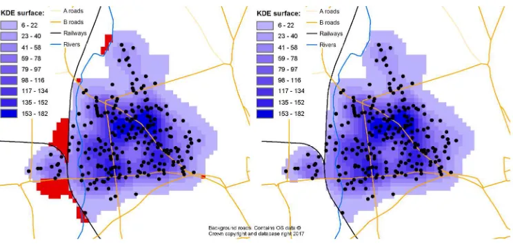
Then, when KDE surfaces are automatically generated (as described in the previous section) only those polygons containing at leastone neighbourhood data point (after the data cleaning and noise reduction processes have been implemented) are made available to the KDE process. This is handled through the use of generating raster grid masks whereby those polygons with relevant neighbourhood point data are assigned a value of 1 and those with no data are assigned a value of 0. The KDE surface is multiplied by the mask to remove those areas where smoothing should not occur. An example of the method is illustrated in Figure 2. The use of linear features as breaklines is represented as a user specified option within the overall automated scripting process.

3.4. Post-analysis synonym identification

While issues related to spellings are dealt with in Section 3.2, there are also cases of neighbourhoods for which synonyms exist - where a completely different word is used to describe the same place (for example ‘New York’ and the ‘Big Apple’ or ‘Sheffield’ and the ‘Steel City’). This can occur due to the use of different languages. Take for instance the postcode CF3 5EA in Cardiff, Wales. This returns data points relating to both the English naming of ‘St. Mellons’ and the Welsh version of the same place - ‘Llaneirwg’. Here, spelling similarities are of no use, and instead we must examine the similarity of spatial footprint of each neighbourhood. To achieve this we compare every neighbourhood KDE grid with each other. Similarity between every paired grid cell for two grids is measured using linear grid regression1. Grids where the level of variance explained (R-squared) was greater than 90% were merged. Output is of interest to both synonym identification and also as a test of geographic similarity between neighbourhoods.

4. Case Study Results

This methodology was applied to the postcodes of the twenty-three case studies (as described in Section 3). During this process a total of 140,856 postcodes were sent to the Bing API, producing 2,182,558 data points. Of these, 366,316 contained additional information between the street name and settlement, which were used to generate a total of 550 neighbourhoods.

Summary statistics are detailed in Supplementary on-line Table S1 to provide an under-standing of the nature of the data and demonstrate that data volumes varied considerably

2_{Such data can be freely downloaded as OS Open data such as OS Open Roads, OS Open Rivers, Meridian}TM₂

from https://www.ordnancesurvey.co.uk/opendatadownload/products.html

1_{Using the Python numpy.polyfit function, and only using cells where data exists in one of the two grids being}

analysed

For Peer Review Only

across each case study - predominately as a reflection of the population size of each area. For example, input data volumes ranged from the 64,349 postcodes (including historic postcodes) within the study areas of Camden and Westminster (London) to just 540 postcodes in Ludlow. These data generated 143 neighbourhoods in Camden and West-minster and just a single neighbourhood in Ludlow. Although each neighbourhood was generated from an extremely varied number of data points, on average a neighbourhood contained 666 data points.

The number of data points returned by the method for neighbourhoods is highly skewed (as shown in Supplementary on-line Figure S1). The potential issue of neighbourhoods with low numbers of data points was overcome by one of the rules required for neigh-bourhood generation (as described within the methodology section) whereby a minimum of 40 data points were required in order to ensure robust mapping.

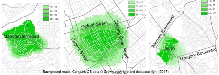
For purposes of illustration, examples of the grids produced by the automated pro-cedures are shown in Figure 3. The percentage grids (Figure 3d, e and f) demonstrate probabilistic output reflecting the probability that at the particular location someone would consider the space as a given neighbourhood name.

An example of combining each extracted neighbourhood into a single file is illustrated in Figure 4 for the city of Sheffield, with eachcombinationof neighbourhoods being shown in a different colour (for example in the north-west corner: areas defined as Stocksbridge are coloured green, areas called Deepcar are in light red and those areas that are referred to as both Stocksbridge and Deepcar are coloured blue. The size of the labels are dependent on the number of data returns for each neighbourhood name).

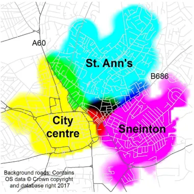
Figure 4 highlights a valuable contribution of our method - it provides the capability to identify areas where perceptions vary and neighbourhood names are contested by different people or organisations. This is illustrated specifically in Figure 5, which shows an example of the differing views of where three neighbourhoods within Nottingham lie. In order to assess the composition of the source of the neighbourhood data, all 121,154 data points relating to the Nottingham case study were manually assigned based on their URL. Two main categorises emerged with 54% originating from business sources and 14% from real estate sources, with the remaining 32% of data points falling outside these two categorisations. Business sources included company reports, credit scores or company director information sites. It is important to stress that much of this data consisted of entries from local trade-persons registered at their home address (electricians and plumbers for example). The residual category included council and governmental documentation, social media sites and personal blogs.

5. Validation

The value of these case studies is that they also provide a basis for assessing the validity of this technique. Specifically, in this section we explore the extent to which neighbour-hoods generated fromweb based content are representative of those derived from asking people directly. Ideally validation would compare output against a complete coverage of resident views. Collecting such data, however, for any extensive geographic area is pragmatically impossible. Furthermore, anysample of resident opinions in itself may not accurately reflect the true underlying representation of neighbourhoods. For this reason, the traditional use of precision and recall would not be suitable.

Two forms of validation exist: (i) validation against existing gazetteers based solely on neighbourhood name and (ii) validation of the neighbourhood geographic extents.

For Peer Review Only

To assess both of these the cities of Nottingham and Sheffield were focused upon, due to the authors having a good local knowledge of their neighbourhoods. Such qualitative information can prove insightful when drawing distinctions between differing perspectives of the various data sources and potential ‘errors’.

5.1. Validation for neighbourhood names

It is possible (and relatively simple) to compare the neighbourhood names generated by our approach against a composite picture derived from multiple gazetteer sources (OSM, OS data1, Yahoo! Geoplanet, Geonames and local council derived neighbourhood names2). This process is straightforward due to the fact that comparisons are solely based on the presence and absence of names within the different sources. Neighbourhoods that are cited by a number of different sources are more likely to be the more significant areas within a particular town or city - hence the level of source agreement is an important measure. However, given that these sources are known to be incomplete (Brindleyet al.

2014), the degree to which data from the method (titled web extraction output) can generate a superset of their contents is important.

In the case of Nottingham - only 3.2% of the combined total of 126 neighbourhood names were contained within all the different sources, 46% were in three or more sources and only 69.8% of neighbourhoods were identified by at least two of the five sources. In comparison, within Sheffield - only 6.0% of the combined 283 neighbourhood names were contained within all six different sources, 40.3% were in three or more sources and only 49.8% of neighbourhoods were identified by at least two of the six sources. This means that in Nottingham and Sheffield, 30.2% and 50.2% of neighbourhoods respectively, were found only in a single source. Such figures demonstrate the low level of general agreement between the different data sources for neighbourhoods.

There were over 3.7 times more neighbourhoods identified by just a single source in Sheffield than compared to Nottingham, the vast majority of which (73%) were found solely in OS data (n=104). Whilst some represent relatively well-known neighbourhoods not included in the other non-OS data (such as Owlerton and Templeborough), a sub-stantial proportion appeared to relate to very small geographical places nested within larger entities. It is highly unlikely that if residents were asked which part of the city or town they lived in that they would provide such names as an answer and would probably cite the larger neighbourhoods that these minutiae nest within. Examples of such cases (in Sheffield) include Den Bank, Wadsley Grove, Carsick, Stephen Hill and Howard Hill. Whilst these do not represent data errors, they are not necessarily of a suitable scale to (1) be well known to other residents of the town or city to have general applicability and (2) might not be robust enough (due to their size) to accurately map and aggregate other socio-economic data to. A number of these smaller areas also appear to relate to historic names that people might not necessarily use in reference to their current neighbourhoods. Given the poor level of comparability between existing gazetteers, perfect agreement with web extracted neighbourhoods is of course unlikely. This said, the degree of overlap is particularly encouraging. Table 1 illustrates that the web extracted output specified 95.5% of the total number of neighbourhoods identified in Nottingham (n=88) when agreement was limited to neighbourhoods found in at least two of the five different

1_{Compromising of a combination of the 50k gazetteer, VectorMap Local and data extracted from the internal}

company data of the Multi Resolution Data Programme (MRDP)

2_{Delineated by Sheffield City Council for policy analysis (Thomaset al.2009) and thus only available for the city}

of Sheffield case study

For Peer Review Only

gazetteers. In comparison, of 121 neighbourhoods defined by the web extraction output in Sheffield 93.0% were also found in at least three of the six existing sources. Table 1 also contains the level of comparability between web extraction output and all neighbourhoods identified with a varying degree of agreement between the different data sources.

Table 1 demonstrates that the two most comprehensive sources are the OS and web extraction output. Given that the OS source is actually a combination of three different datasets, if a single gazetteer were to be used the web extraction output would be a clear winner, consistently containing the highest level of agreement with the other sources.

A complete list of the 25 neighbourhoods identified by the web extraction output (in Nottingham or Sheffield), but not found in the other gazetteer sources, can be found in Table 2. Other evidence of each omitted neighbourhood’s existence was gathered for the majority of cases: from within a different class within OSM (for example as an ‘Industrial Area’ rather than specifically as a ‘suburb’); as ancillary features in OSM (occurrences of near-by objects, including for example, bus stops, village greens, named building and so on, that share the neighbourhood name); or from references in historical OS maps.

This provided further evidence for the validity of all but seven web generated neigh-bourhoods. These are shown with asterisks in Table 2 (five in Nottingham and two in Sheffield). Of these, there is little doubt, for example that the City centre actually exists and is not a data error issue, despite most neighbourhood level gazetteers not including it. Similarly, Clifton Estate was at one time the largest council estate in Europe1 and its existence is without question. Its omission from gazetteers is likely due to the fact that when asked, many may refer to the area generically as Clifton (rather than the sub-neighbourhood of Clifton Estate). There is also a substantial body of on-line material relating toHeronridge (also called Heron Ridge) compromising of house details on estate agent websites, local businesses carrying the name, along with mentions on Wikipedia1 and council documentation2. Similarly, there are a number of references

to ‘Victoria Business Park, Netherfield’ on the Web, including references in local

government documentation3. Although no references to ‘Warren Hill’ can be found in historic OS maps - there is text annotation citing The Warren and Warren House. There are also a large number of websites listing Warren Hill, including a residents’ association which is recognised by the local council4.

In Sheffield, there are no references to ‘Parkway Industrial Estate’ within old OS maps, although there are references to an ‘industrial estate’ along with descriptions of ‘Parkway Market’ from the 1950s and ‘Parkway Works’ from the 1990s. WhilstWadsley

Park Village(built on the former site of Middlewood Hospital between 2001 and 2006)

does not appear in any of the existing neighbourhood gazetteers, the area does have its own community website and forum5. There appears supporting evidence for all the areas that were identified by the web extraction output but not found within other gazetteer sources - demonstrating the incompleteness of existing sources of neighbourhoods within current gazetteers and supporting the need for additional methods of identification.

There were 12 neighbourhoods that existed in gazetteers but which were not identi-fied by web extraction. These can be found in Table 3. It should be stressed that this

1_{http://en.wikipedia.org/wiki/Clifton, Nottingham} 1_{http://en.wikipedia.org/wiki/Bulwell}

2

http://committee.nottinghamcity.gov.uk/Data/City%20Council/20070716/Agenda/$070625%20-%2028623.doc.pdf

3_{http://www.gedling.gov.uk/media/documents/planningbuildingcontrol/localplanningdocument/Gedling}

%20Growth%20Strategy%20Employment%20Site%20Assessments.pdf

4_{http://warrenactiongroup.org and https://democracy.gedling.gov.uk/mgOutsideBodyDetails.aspx?ID=249} 5_{http://www.wpvonline.co.uk}

For Peer Review Only

represents a very small proportion (5.5%) of the total number of areas that the method identified. Whilst all of these were to be found within the data output (as expressed by the frequency column within Table 3) they contained very low numbers of data points and were therefore not consideredrobust enough to be included in further analysis.

5.2. Validation for neighbourhood geographies

Validation of thegeography of neighbourhoods is more problematic due to the subjective nature and general lack of data for comparisons. Seeking resident opinions provides the closest measure to any potential ground truth. Data were collected for three different scenarios, each with increasing spatial resolution:

• resident views from an on-line questionnaire for places within Nottingham; • information collected from residents by a Neighbourhood Forum; and

• resident views in targeted streets where web extraction output portrayed evidence of differing views of neighbourhood name within the same local space.

Each of these different forms of resident validation will now be discussed in turn.

5.2.1. Residents’ views in Nottingham:

This validation explores resident responses for neighbourhoods in general across the city of Nottingham. Sixty-eight resident views were collected through responses to an online survey where residents were simply asked the ‘name of the area’ in which they lived and their postcode6. Thus, the point location of a resident’s location can be com-pared to the different underlying geographies of neighbourhood that a variety of sources produce (Wikimapia1, Quattroshapes2, OS MRDP3, web extraction output). Addition-ally, resident views were also compared with the Voronoi Diagrams constructed from the other existing neighbourhood centre-point gazetteers (Geonames, OSM and Yahoo! Geoplanet). Such a procedure conceptually compares the resident’s reported neighbour-hood and the closest centre-point from each of the gazetteers. A slight difficulty was encountered due the vague nature of classification within the web extraction output: for example a resident calling an area Bulwell matches even if the web extraction output declares that 99% of data relate to the area as Arnold and 1% as Bulwell. In order to demonstrate the level of likely consensus, cases were identified as a ‘minor’ match if less than 50% of data within the web extraction output were found to agree with the res-ident perspective. This represented 10% (n=7) of resres-ident surveys. A record was also attributed as a ‘minor’ match if the difference was only due to a qualifier such as Lenton andNew Lenton.

The sixty-eight residents provided a total of sixty-six unique postcodes and covered thirty-four different neighbourhoods. The output of the resident view comparisons can be found within Figure 6 and demonstrates the high level of agreement found between residents and the web extraction output, with over an 98% agreement (comprised of 88% where data specified a supporting majority view with the resident and a further 10%

6_{Participants were recruited through a variety of online sources including the twitter accounts of Nottinghamshire}

County Council (https://twitter.com/nottscc), and Nottingham City Transport (https://twitter.com/nct buses) and the Reddit page for Nottingham (http://www.reddit.com/r/nottingham)

1_{An open-content collaborative mapping project that may include neighbourhood boundaries - extracted from}

wikimapia.org

2_{Derived from foursquare checkins and geo-tagged photos from Flickr cross-referenced with Geonames and Yahoo!}

GeoPlanet. Data available from quattroshapes.com as an ESRI shapefile

3_{As described in Section 5.1}

For Peer Review Only

agreement but as a minority representation). There was no agreement in just one of the sixty-eight cases - where the resident postcode and specified neighbourhood was actually over 3km away from the corresponding area identified by the web extraction output. Given this large distance and the fact that similar disparities were also found between this particular resident view and the other sources, the postcode supplied by the resident in this case is likely to be incorrect4_.

The web extraction output outperformed all of the other sources in terms of agreement with resident views. Both the Wikimapia and OS MRDP in comparison only agreed in approximately 70% of cases, whilst the remaining sources fared worse with agreement in only 30-40% of residents surveyed.

The Voronoi diagrams used when surveying residents’ opinions represented discrete boundary information - a best guess based on the neighbourhood centre-points provided by gazetteers. In contrast the web extraction output are represented by a vague repre-sentation (300m KDE smoothings). If a similar KDE measure had been applied to the gazetteers centre-point data, the level of matching (between the Voronoi diagram output and 68 resident views) would actually have got worse. This is primarily due to the small geographic scale of areas within 300m of the gazetteer centre-points. Of the eight resident views within 300m of OSM gazetteer centre-points, 25% were incorrect (with a further 25% producing a minority view). Yahoo! Geoplanet and Geonames performed worst, with 50% of resident views being incorrectly identified in both cases (with a sample size of eight surveyed resident perspectives within 300m for the Yahoo! Geoplanet data and only two for Geonames). Thus, the poor agreement between resident views and Voronoi Diagram output from gazetteer centre-points, compared to the levels of agreement from the web extraction output, do not appear to be due to methodological differences.

A large proportion of resident data (nearly 15%) found no comparison with Wikimapia due to lack of neighbourhood data within Wikimapia, demonstrating the difficultly in achieving full coverage through active crowdsourcing. It should also be noted that in a number of cases, residents’ views were to be found in close-by neighbourhoods within Wikimapia. In this regard, there were nine cases where agreement with the resident view were found within 300 metres. Even allowing for these relatively ‘near-misses’, however, the level of agreement would still only stand at 87% - some way shy of the 98% found for the web extraction output.

5.2.2. Information collected by a Neighbourhood Forum:

It is possible to specifically examine the detailed geography of an individual neigh-bourhood if enough resident responses can be collected. To this end, we performed a comparison based on 329 data points that were gathered by the Neighbourhood Forum of Crouch End (London) via a field survey. Individuals at a local community arts fes-tival for the area were asked to mark their home location with a colour coded sticker representing different neighbourhood names within the area.

Resident perceptions of this neighbourhood could then be compared to a set of al-ternative data extents (as applied within Section 5.2.1) - in this case boundaries from Wikimapia, OS MRDP, Quattroshapes and the web extraction output. Figure 7 maps out the comparison, with Table 4 providing a summary view. Results demonstrate that the web extraction dataset was considerably closer to resident perceptions than any of the other data. Not only did the web extraction output produce the highest level of agreement with resident perspectives, by a significant margin (76% compared to the next highest

4_{A correction of one digit from a 4 to a 9 could potentially explain the effect}

For Peer Review Only

data source of only 35%), but also returned the smallest level of cells identified by the residents but not included within the output from the specified method (false-positives and false-negatives).

5.2.3. Testing differing perspectives within the same localised space:

By targeting areas where the web extraction output purports to show divergent vari-ations in the neighbourhood name for a given space, it is possible to validate the data by comparing the name of the neighbourhood when asking residents their views and opinions. In order to validate the data, one would expect the same differences in opinion to occur in both the web extraction output and resident responses. To this end, opinions were sought by visiting residential properties in three postcodes in Sheffield (S10 1FA -Roslin Road; S10 1BJ - Crookesmoor Road; and S10 5BD - Crookes Road) and residents were asked the name of the area that they lived in. The three streets were chosen as they appear (in the web extraction output) to sit of the intersection of three different neighbourhoods (Broomhill, Crookes and Crookesmoor).

The responses demonstrated the highly variable nature of neighbourhoods, with fre-quently neighbours possessing different views with little spatial cohesion. The data are tabulated in Table 5 along with the comparative output from the web extraction method. It is noteworthy that in one instance even people living in the same property had different opinions on the name of their local area.

The appropriateness of a Chi-square test is dependant on having enough data points. Given the small numbers associated with individual postcodes (approximately 15 prop-erties), it is highly likely that, given response rates and dividing data points between a number of differing neighbourhoods, there would be insufficient data points for a Chi-square test at the postcode level. Thus, in order to meet the assumptions of the test, data were aggregated for all three postcodes in order to investigate any differences between the output from the web extraction method and resident responses. Data aggregation in this case was acceptable due to the close proximity of the postcodes, with them covering an area of just over one hectare in size. No statistically significant difference was found between the web extraction output and resident responses (X2 = 0.09, df = 2, p <0.05). This has two important implications as it not only aids the validation of the web ex-traction output (being similar to that when asking residents directly) but also more fundamentally supports the notion and requirement of vague neighbourhood boundaries. If a more accurate representation is required - the fact that people even within the same property can have such varying views1 demonstrates that discrete boundaries can never capture such complexity and vague notions are necessary.

6. Discussion

6.1. Strengths of the study

Evidence indicates that at an absolute minimum, the proposed web extraction method-ology could extend the comprehensiveness of neighbourhood level gazetteers. Crucially, however, this automated procedure also does not require the names of the units of in-terest to be known a priori. The tight delimitation between street and city elements

1_{In this instance the residents stressed the importance of status of belonging to certain neighbourhoods as the}

ra-tionale for differences of opinion within the household. Whilst of pertinent interest to future work, the investigation ofwhy people identify with different neighbourhood names was considered outside the scope of this work

For Peer Review Only

reduces issues of ambiguity, facilitating for example the clear disjuncture of references to ‘Birley’ (Sheffield) from those of ‘Birley Carr’ (Sheffield). The successful validation study demonstrated that ‘neighbourhoods’ extracted in an automated fashion from the Web are indeed representative of neighbourhoods more generally - and as such do not represent some special subset of these social units.

Furthermore, the work highlights the usefulness of using the percentage of data returns that relate to a named neighbourhood (in addition to the usual absolute number of data returns). Whilst the absolute data maps (Figures 3 a, b and c) identify concentrations focused around the core (commonly shopping areas) of the neighbourhoods, the percent-age maps (Figures 3 d, e and f) for the corresponding areas exhibit a rather different geography, identifying where the majority of people may associate with the neighbour-hood names. For instance, compare the differences for the area to the north of Crosspool (Sheffield) labelled with anx in Figures 3 a and d where data volumes may be low but there is overall consensus that the area is defined as ‘Crosspool’. Such measures are ex-tremely insightful where data volumes might be expected to be low (for example on the periphery of towns and cities, near rivers, or in close proximity to large parks).

When multiple neighbourhood KDE surfaces are overlaid (such as in Figure 5) it is possible to denote areas whereby people within a synonymous space may have varying points of view of what the area may be named. Consequently, this ties with the require-ment to identify ‘vague’ perceptions of neighbourhood. Although we all have individual opinions of the areal extent of neighbourhood areas, it is only when examined collectively that sense can be deduced (for example this is where the majority of people believe x might be). Disjuncture along specific roads are evident in Figure 5 and demonstrate the value of the hard break-line procedure. There is some spreading of Sneinton north of the B686 (Carlton Road) into St. Ann’s but St. Ann’s does not appear to extend south of the B686. Similarly, the yellow tones to the south-west of the A60 indicate no mixing - with people appearing to only identify with the area as the City Centre (with no references to St. Ann’s). In contrast, the green tones to the north-east of the road denote perceptions of both St. Ann’s and the City Centre being present. The dynamic nature concerning whether neighbourhoods extend beyond specific linear features vindicates the innovative use of hard break-lines within neighbourhood delimitation through KDE.

There is also potential of the output from this research to assist with Neighbourhood Planning. Neighbourhood Planning came into effect in the UK in April 2012 through the 2011 Localism Act and aims to give communities and local groups more power within the planning process. Before producing a Neighbourhood Plan, a local group is required to propose a boundary for the area. In this context, planning officers within Sheffield City Council were able to assess the level to which proposed neighbourhood areas from local groups compared with the neighbourhood spaces extracted from web content.

6.2. Weaknesses of the study

It should be stressed that the approach adopted in this paper rests on the use of postal addresses held on the Internet. Whilst this brings a number of advantages, including high data volumes of user generated content, there are also limitations. Due to the nature of the input data, neighbourhood content can not be derived for unpopulated spaces, such as parks or other natural environments. Thus, the method is most appropriate when the focus rests on populated areas. For example, aggregating Census information to the neighbourhood names and spaces to which people use and relate to. Future work could explore the potential of combining neighbourhood level content derived from web based

For Peer Review Only

postal addresses with Flickr data, in order to resolve this shortcoming.

There is little control over the input data as it is gathered from the Web. It may be the case that an element of the raw input data (from the Web) are generated by some semi-automatic process. In such examples, our method would reverse engineer those geographic extents. Whilst this is entirely possible, there is a high level of agreement between the proposed method and resident views (sections 5.2.1, 5.2.2 and 5.2.3), with the approach outperforming the alternative data sources. This would suggest that the extent of such practices are unlikely to be critically influencing the output of our data.

Whilst it would be perfectly possible to generate vague boundaries in more rural con-texts (for example for villages), the strength of the method is that official addressing conventions in the UK do not require urban neighbourhood information. Thus, any neigh-bourhood references must be some form of user content. In contrast, in rural areas, output would merely be a reflection of Royal Mail’s official recording practises.

Adaptive kernel density estimation could be used to define KDE parameters automat-ically, based on the original underlying point data. Such methods are particularly suited where: (1) the objects of concern vary in geographic scale; or (2) there is considerable variation in the context in which the objects of concern are found (for example contrasts in population density between urban and rural areas). Whilst neither of these issues are of primary concern for this work (the focus rests with neighbourhoods within an urban context), the use of adaptive parameters would alleviate the limitation within the cur-rent method which requires the use of a number of thresholds within the process. The incorporation of adaptive kernel density estimation was, however, considered outside the scope of this paper but should form the basis for future work in this field.

Although this work has been applied within the UK, such an approach could be utilised elsewhere providing that the postal delivery service in the country facilitated the use of additional information within the address. In many countries, however, such as Brazil, the postal delivery system is more rigid than found in the UK and only administratively assigned, official names, are found in postal addresses - even those found on the Web. In such cases, the method outlined here would be of little value. In some contexts it may be possible to identify certain features but not all neighbourhoods. For example, whilst data in New Zealand generally follows administratively assigned names, it is possible to extract data concerning the CBD (which is not an official postal description). Similarly in the USA, references to Downtown may be found after the Zip code. The approach may be of value in countries with burgeoning address systems where reference to neighbourhoods are common (in Dar es Salaam, Tanzania for example). Whilst there is potential to adopt similar techniques within different countries, a detailed knowledge of the local circumstances would be required. Thus, there remains a need to explore the extent to which the method might be applied on a case-by-case basis.

7. Conclusion

This research has been able to demonstrate the feasibility of mapping vague neighbour-hood boundaries in the UK by combining linguistic models with data gathered through the passive mining of postal addresses held on the Web. Thus, it is possible to construct highly scalable, vague definitions of UK neighbourhoods that can be used as the sub-strate for business, policy and social decisions. Whilst the method developed here will not be universally applicable across the globe (due to variations in postal addressing conventions), the approach demonstrates value even if the technique can only be applied

For Peer Review Only

within specific contexts. The paper has also revealed the incompleteness within current neighbourhood level UK gazetteers - which has important consequences for studies iden-tifying neighbourhoods using cross-referencing procedures with a single gazetteer. Future work should seek to address this by exploring the potential of combining neighbourhood level data across multiple gazetteers. The paper has highlighted innovation within KDE processes - with the use of hard break-lines and different bandwidths for data cleaning. Furthermore, this work has shown the plausibility of automatically mapping vague UK neighbourhood extents without prior knowledge of the neighbourhood names themselves. Even with this relatively simple initial method, the potential of combining Web-based data with linguistic models to produce viable geospatial intelligence is evident.

8. Acknowledgements

The primary author was supported by the Horizon Centre for Doctoral Training at the University of Nottingham [RCUK Grant No. EP/G037574/1] and by the RCUK’s Horizon Digital Economy Research Institute [RCUK Grant No. EP/G065802/1]. We thank the anonymous reviewers who provided helpful comments on earlier drafts of the manuscript.

References

Bibby, P.R. and Shepherd, J., 2004. Developing a new classification of ur-ban and rural areas for policy purposes: the methodology. [online] Avail-able from: https://www.gov.uk/government/statistics/2001-rural-urban-definition-la-classification-and-other-geographies [Accessed 5 June 2017].

Brindley, P., 2016. Generating Vague Geographic Information through Data Mining of Passive Web Data. Thesis (PhD). School of Computer Science, The University of Nottingham, UK.

Brindley, P., Goulding, J., and Wilson, M.L., 2014. A Data Driven approach to map-ping urban neighbourhoods.In:ACM International Conference on Advances in GIS (SIGSPATIAL), Nov. 4-7th., Dallas, Texas, USA, 437–440.

Buscaldi, D., 2011. Approaches to disambiguating toponyms.SIGSPATIAL Special (Let-ters on Geographic Information Retrieval), 3 (2), 16–19.

Clasper, L., 2017. Exploring vernacular perceptions of spatial entities: Using Twitter data and R for delimiting vague, informal neighbourhood units in Inner London, UK.In:Proceedings of VGI-Analytics 2017, May 9th., Wageningen University, The Netherlands at AGILE 2017.

Cranshaw, J.,et al., 2012. The Livehoods Project : Utilizing social media to understand the dynamics of a city. In: Sixth International AAAI Conference on Weblogs an Social Media (ICWSM 2012), June 4-7th., Trinity College in Dublin, Ireland, 58– 65.

de Smith, M., Goodchild, M., and Longley, P., 2007. Geospatial Analysis: A Compre-hensive Guide to Principles, Techniques and Software Tools. Troubador Publishing Ltd: Leicester.

Flemmings, R., 2010. Revealing the Fuzzy Geography of an Urban Locality.In:GIS RE-SEARCH UK (GISRUK), Proc. Of the GIS Research UK 18th Annual Conference, April 14-16th., London, UK, 345–351.

For Peer Review Only

Galster, G., 2012. The Mechanism(s) of Neighbourhood Effects: Theory, Evidence, and Policy Implications. In: M. van Ham, D. Manley, N. Bailey, L. Simpson and D. Maclennan, eds. Neighbourhood Effects Research: New Perspectives. Springer Netherlands, 23–56.

Grothe, C. and Schaab, J., 2009. Automated footprint generation from geotags with kernel density estimation and support vector machines.Spatial Cognition and Com-putation, 9 (3), 195–211.

Hall, M.M. and Jones, C.B., 2008. A field based representation for vague areas defined by spatial prepositions. In:Proceedings of Methodologies and Resources for Processing Spatial Language, Workshop at LREC’2008.

Hollenstein, L. and Purves, R.S., 2010. Exploring place through user-generated content: Using Flickr to describe city cores.Journal of Spatial Information Science, 1, 21–48. Jones, C.B., et al., 2008. Modelling Vague Places with Knowledge from the Web.

Inter-national Journal of Geographical Information Science, 22 (10), 1045–1065.

Keßler, C., Janowicz, K., and Bishr, M., 2009. An agenda for the next generation gazetteer: Geographic information contribution and retrieval.Proceedings of the 17th ACM SIGSPATIAL International Conference on Advances in Geographic Informa-tion Systems - GIS09, 91–100.

Leidner, J. and Liberman, M., 2011. Detecting Geographical References in the Form of Place Names and Associated Spatial Natural Language.In: R. Purves and C. Jones, eds. Letters on Geographic Information Retrieval., 5–12.

Li, L. and Goodchild, M.F., 2012. Constructing places from spatial footprints. Proceed-ings of the 1st ACM SIGSPATIAL International Workshop on Crowdsourced and Volunteered Geographic Information - GEOCROWD ’12, 15–21.

Lynch, K., 1960.Image of the City. The MIT Press: Cambridge MA, USA.

Montello, D.R.,et al., 2003. Where’s Downtown?: Behavioral Methods for Determining Referents of Vague Spatial Queries.Spatial Cognition & Computation, 3, 185–204. Moulaert, F.,et al., 2007.Can Neighbourhoods Save the City?: Community Development

and Social Innovation (Regions and Cities). Routledge: London.

Orford, S. and Leigh, C., 2013. The Relationship between Self-reported Definitions of Urban Neighbourhood and Respondent Characteristics: A Study of Cardiff, UK.

Urban Studies, 51, 1891–1908.

Pickles, E., 2010. Eric Pickles’ speech to the Local Government As-sociation annual conference, 7 July 2010. [online] Available from:

https://www.gov.uk/government/speeches/local-government-association-conference-6-july-2010 [Accessed 5 June 2017].

Popescu, A., Grefenstette, G., and Mo¨ellic, P.A., 2008. Gazetiki: Automatic Creation of a Geographical Gazetteer.In:Proceedings of the 8th ACM/IEEE-CS Joint Conference on Digital Libraries, JCDL ’08, Pittsburgh, USA, 85–93.

Purves, R.S., Clough, P., and Joho, H., 2005. Identifying imprecise regions for geographic information retrieval using the web. In: Proceedings of GIS RESEARCH UK 13th Annual Conference, Glasgow, UK, 313–318.

Purves, R.S., et al., 2007. The design and implementation of SPIRIT: a spatially aware search engine for information retrieval on the Internet. International Journal of Geographical Information Science, 21 (7), 717–745.

Sampson, R.J., 2012. Moving and the Neighborhood Glass Ceiling.Science, 337, 1464– 1465.

Schockaert, S., 2011. Vague regions in Geographic Information Retrieval. SIGSPATIAL Special (Letters on Geographic Information Retrieval), 3 (2), 24–28.

For Peer Review Only

Schockaert, S. and De Cock, M., 2007. Neighborhood restrictions in geographic IR. Pro-ceedings of the 30th annual international ACM SIGIR conference on Research and development in information retrieval - SIGIR ’07, p. 167.

Thomas, B., et al., 2009. A tale of two cities: the Sheffield project. A report by the Social and Spatial Inequalities Research Group University of Sheffield, Sheffield. [online] Available from: http://sasi.group.shef.ac.uk/research/sheffield [Accessed 5 June 2017].

Thurstain-Goodwin, M. and Unwin, D., 2000. Defining and Delineating the Central Ar-eas of Towns for Statistical Monitoring Using Continuous Surface Representations.

Transactions in GIS, 4 (4), 305–317.

Twaroch, F.A., Jones, C.B., and Abdelmoty, A.I., 2008. Acquisition of a vernacular gazetteer from web sources. Proceedings of the first international workshop on Lo-cation and the web - LOCWEB ’08, Beijing, China, 61–64.

Twaroch, F.A., Jones, C.B., and Abdelmoty, A.I., 2009a. Acquisition of Vernacular Place Names from Web Sources. In: R. Baeza-Yates and I. King, eds. Weaving Services and People on the World Wide Web. Springer Berlin Heidelberg, 195–214.

Twaroch, F.A., Purves, R.S., and Jones, C.B., 2009b. Stability of Qualitative Spatial Relations between Vernacular Regions Mined from Web Data. In: Proceedings of Workshop on Geographic Information on the Internet, Toulouse, France, April 6th. Vallee, J.,et al., 2015. The ‘constant size neighbourhood trap’ in accessibility and health

studies. Urban Studies, 52 (2), 338–357.

Vasardani, M., Winter, S., and Richter, K.f., 2013. Locating place names from place descriptions. International Journal of Geographical Information Science, 27, 2509– 2532.

Wilson, R., 2009. Why neighborhoods matter: the importance of geographic composition.

Geography and Public Safety, 2 (2), 1–2.

Zhang, A.X., et al., 2013. Hoodsquare: Modeling and recommending neighborhoods in location-based social networks.ArXiv e-prints.

For Peer Review Only

Sources in agreement: 1 2+ 3+ 4+ 5+ 6+

1 source only) Nottingham:

web extraction output 81.0 95.5 98.3 100.0 100.0 n/a 98.4 OS combined 73.8 93.2 98.3 100.0 100.0 n/a 97.9 Yahoo! Geoplanet 34.1 45.5 63.8 84.0 100.0 n/a 73.3 OSM 30.2 39.8 51.7 88.0 100.0 n/a 69.9 Geonames 19.8 25.0 37.9 44.0 100.0 n/a 51.7 Sheffield:

OS combined 83.0 92.9 94.7 100.0 100.0 100.0 97.5 web extraction output 42.8 80.9 93.0 96.3 100.0 100.0 94.0 OSM 43.5 79.4 90.4 98.8 100.0 100.0 93.7 Council defined 36.4 65.2 75.4 91.3 89.7 100.0 84.3 Yahoo! Geoplanet 14.8 28.4 32.5 42.5 79.5 100.0 56.6 Geonames 17.7 30.5 33.3 41.3 74.4 100.0 55.9

For Peer Review Only

Neighbourhood name web extraction output

Found in OSM Historic OS maps Nottingham:

*City Centre 274 No No Queens Drive Industrial Estate 225 Yes - different class No Hockley 190 Yes - ancillary features Yes Blenheim Industrial Estate 182 Yes - different class No Lenton Lane Industrial Estate 173 Yes - different class No Papplewick 135 Yes - ancillary features Yes *Clifton Estate 135 No No Canning Circus 122 Yes - ancillary features Yes Old Market Square 92 Yes - ancillary features Yes Clifton Village 91 Yes - ancillary features No Chetwynd Business Park Chilwell 86 Yes - different class No Colwick Park 58 Yes - ancillary features Yes Castle Boulevard 51 No Yes Wilford Village 50 Yes - ancillary features No *Heronridge 50 No No *Victoria Business Park Netherfield 50 No No Boulevard Industrial Park Beeston 49 Yes - different class No *Warren Hill 42 No No Sheffield:

Holbrook Industrial Estate 347 No Yes Hunters Bar 323 Yes - different class Yes Meadowhall Centre 228 Yes - different class Yes Newhall 75 No Yes *Parkway Industrial Estate 61 No No *Wadsley Park Village 61 No No Thorncliffe Park, Chapeltown 44 Yes - different class No

For Peer Review Only

Neighbourhood name Frequency ... Neighbourhood name Frequency Nottingham: Sheffield:

Bulwell Forest 9 Batemoor 21 Highbury Vale 30 Carbrook 36 Porchester 12 Greenland 20 Standard Hill 1 Hemsworth 16 Herdings 29 Hollins End 10 Lowfield 11 Park Hill 25

For Peer Review Only

Cell count % Cell count % Cell count % Cell count % Agreement between

resident data and output from alternative methods). Similar to ‘True positives’ if resident sample was ground truth

1,072 76.1 516 34.7 385 22.6 414 27.1 No resident support

(method identifies area but no supporting resident evidence). Similar to ‘False positives’ if resident sample was ground truth

54 3.8 132 8.9 348 20.4 170 11.1 Resident view only (method

failures to capture resident defined areas). Similar to ‘False negatives’ if resident sample was ground truth

283 20.1 839 56.4 970 57.0 941 61.7

For Peer Review Only

Broomhill 3 3 60.0 50.0

Crookesmoor 2 2 40.0 33.3

Crookes 0 1 0.0 16.7

Total response rate: 5 from 19 26.32

b) Crookesmoor Road: Web extraction

output

Asking residents

% Web extraction output

% Asking residents Broomhill 3 3 50.0 60.0

Crookesmoor 3 2 50.0 40.0

Total response rate: 5 from 9 55.56

c) Crookes Road: Web extraction

output

Asking residents

% Web extraction output

% Asking residents Broomhill 15 9 75.0 75.0

Crookes 5 3 25.0 25.0

Total response rate: 10 from 20 50.00

For Peer Review Only

List of Figure captions:

Figure 1. Identifying example neighbourhood terms between street and settlement content based on a search for the postcode NG7 1LS within an internet search engine such as Google or Bing

Figure 2. Linear features as breakline constrains for smoothing (KDE legends = number data points within 300m): Example of Radford, Nottingham

a) KDE (Absolute data, 300m bandwidth)... b) Mask: green = where smoothing allowed

c) Fig(a)*Fig(b): blue = areas masked out....d) Final modified KDE (300m bandwidth)

Figure 3. Examples of generated vague neighbourhood boundaries

Absolute 300m KDE grids (legend = number data points within 300m) for: a) Crosspool, Sheffield b) Soho, London c) Bobbers Mill, Nottingham

Percentage 300m KDE grids (legend = proportion of data within 300m radius supporting the neighbourhood name) for: d) Crosspool, Sheffield e) Soho, London f ) Crosspool, Nottingham

Figure 4. Example data output: Sheffield neighbourhoods

Figure 5. Cyan-Magenta-Yellow (CMYK) composite, demonstrating differing perceptions of three neighbourhoods in Nottingham

Figure 6. Comparison of sixty-eight resident views in Nottingham with different sources of neigh-bourhood geography

Figure 7. Level of geographic agreement between resident perceptions for Crouch End (London) with a range of other data output

.a) Web extraction data comparison data...b) Wikimapia data comparison...

...c) OS MRDP data comparison... d) Quattroshapes data comparison...

Figure S1. Neighbourhood data point distribution

For Peer Review Only

Figure 1. Identifying example neighbourhood terms between street and settlement content based on a search for the postcode NG7 1LS within an internet search engine such as Google or Bing

102x48mm (300 x 300 DPI) 4

For Peer Review Only

Figure 2. Linear features as breakline constrains for smoothing (KDE legends = number data points within 300m): Example of Radford, Nottingham

a) KDE (Absolute data, 300m bandwidth) b) Mask: green = where smoothing allowed

203x91mm (299 x 299 DPI)

For Peer Review Only

Figure 2. Linear features as breakline constrains for smoothing (KDE legends = number data points within 300m): Example of Radford, Nottingham

c) Fig(a)*Fig(b): blue = areas masked out d) Final modified KDE (300m bandwidth)

203x91mm (299 x 299 DPI)

For Peer Review Only

Figure 3. Examples of generated vague neighbourhood boundaries Absolute 300m KDE grids (legend = number data points within 300m) for:

a) Crosspool, Sheffield b) Soho, London c) Bobbers Mill, Nottingham

166x58mm (299 x 299 DPI) 4