Inference on factor structures in heterogeneous panels

Inference on Factor Structures in Heterogeneous Panels

Carolina Castagnetti

University of Pavia

Eduardo Rossi

University of Pavia

Lorenzo Trapani

Cass Business School, City University London

October 4, 2017

Abstract

This paper develops an estimation and testing framework for a stationary large panel model with observable regressors and unobservable common factors. We allow for slope heterogeneity and for correlation between the common factors and the regressors. We propose a two stage estimation procedure for the unobservable common factors and their loadings, based on Common Correlated E¤ects estimator and the Principal Component estimator. We also develop two tests for the null of no factor structure: one for the null that loadings are cross sectionally homogeneous, and one for the null that common factors are homogeneous over time. Our tests are based on using extremes of the estimated loadings and common factors. The test statistics have an asymptotic Gumbel distribution under the null, and have power versus alternatives where only one loading or common factor di¤ers from the others. Monte Carlo evidence shows that the tests have the correct size and good power. JEL codes: C12, C33.

1

Introduction

Consider the following model for stationary panel data:

yit = 0ixit+ 0ift+ it; (1)

xit = ift+ xit; (2)

where i= 1; :::; n, t= 1; :::; T, xit is anm-dimensional vector of observable explanatory variables andft is anr-dimensional vector of unobservable common factors; in equation (2), i is a matrix of coe¢ cients of dimension m r. Model (1)-(2) is based on Pesaran (30), and it arguably has a huge potential for empirical applications. In the context of …nance,yit could represent the excess return on an asset; then, as pointed out by Bai (3),ftcould represent a vector of unobservable factor returns, which are added to the observable ones (e.g. the Book-to-Market ratio) that are typically employed. Kapetanios and Pesaran (26) consider an APT model allowing for individual asset returns to be a¤ected by common factors (both observable and unobservable). In a similar setup, Castagnetti and Rossi (11) adopt a heterogeneous panel with a multifactor error model to study the determinants of credit spread changes in the Euro corporate bond market. Factor models are also useful in the context of estimating production functions, where

xit is a set of observable factor inputs, and ft allows to consider cross sectional dependence as arising from common shocks or e.g. spillover e¤ects determined by policy or technology shocks. For example, Eberhardt and Teal (17) adopt a common factor model approach to estimate cross-country production functions for the agriculture sector. Similarly, Eberhardt, Helmers and Strauss (16) consider the impact of spillovers in the estimation of private returns to R&D allowing for a common factor framework. Another promising …eld of application is the prediction of mortality rates (or their …rst di¤erence), where the seminal Lee-Carter model (28) has been extended to incorporate idiosyncratic explanatory variables as well as the traditional factor structure - see French and O’Hare (21) and the references therein.

Bai (3) develops a di¤erent estimation technique for (1)-(2) under the assumption of homogeneous slopes, i.e. _i = . Such technique is known as the Interactive E¤ect (henceforth IE) estimator, and it is based on iteratively computing for given values of _iandft, and then i andftfor a given value of . Although results are available for the estimated triple ( ; i; ft), inference is developed under the assumption of homogeneous _is; moreover, no explicit asymptotics for _i or ft is derived beyond consistency. Despite this, inference on _i andftis likely to be important in many settings. For instance, where a multifactor error structure is employed for the purpose of dimension reduction, or simply when explanatory variables may not be observable. In such cases, it could be relevant to know whether there is indeed a factor structure in (1), or whether common e¤ects can be adequately represented by more parsimonious models such as a model with cross-sectional or time dummies, as also studied by Sara…dis, Yamagata and Robertson (32), and Bai (3) in the context of model (1) with homogeneous slopes. In this case, the asymptotics of the estimated common factors and loadings is obviously a …rst, fundamental step in order to construct tests for the presence of a multifactor error structure.

This paper makes two contributions to the literature. Firstly, we derive the inferential theory for the unobservable common factorsftand their coe¢ cients i in (1)-(2). We estimate i andftby applying PC to the residuals computed from (1) using the CCE estimator. This two-stage procedure builds on an idea of Pesaran (30, p.1000), and Pesaran and Tosetti (31), while the asymptotics of the estimated ( i; ft)is studied by adapting the method of proof in Bai (3) to the case of heterogeneous is.

slope homogeneity developed by Kapetanios (25) and Westerlund and Hess (34). Monte Carlo evidence shows that the tests have correct size and satisfactory power for di¤erent levels of the signal-to-noise ratio and for several simulation designs.

The paper is organized as follows. The estimation procedure, and the asymptotics of the estimates of _i andftare in Section 2; Section 3 contains results about the two tests mentioned above. Section 4 contains a validation of our theory through synthetic data. Section 5 concludes. All proofs are provided either in the Appendix or in Castagnetti, Rossi and Trapani (2014).

NOTATION. We use “ !” to denote the ordinary limit; “ d!” and “ p!” to denote convergence in distribution and in probability respectively; and we use “a.s.” as short-hand for “almost surely”. The Frobenius norm of a matrixAis denoted askAk=ptr(A0_{A), wheretr(A)denotes the trace ofA.} De…nitional equality is denoted as “ ”. Other notation is de…ned throughout the paper and in Appendix.

2

Estimation

In model (1)-(2), where xit is m-dimensional and ft is r-dimensional, we consider the following no-tation, which we use throughout the whole paper. We de…ne F = (f1; :::; fT)

0

; Xi = (xi1; :::; xiT) 0

;

i = ( i1; :::; iT)0;yi= (yi1; :::; yiT)0;zit= (yit; x0it) 0

; zi= (zi1; :::; ziT)0 and Hw=n 1Pn_i=1zi. We also de…ne the matricesMw=IT Hw Hw0 Hw

1

H_w0 and

Ci= [ ij 0 i]

2 6 4

1 01 m i Im

3 7 5;

for each i. Based on this, the _is in (1) can be estimated as

~ i=

X_i0MwXi

T

1

X_i0Mwyi

T ; (3)

which is the CCE estimator of Pesaran (30); it holds that ~i i =Op p1_T +Op p_nT1 +Op _n1 .

In order to estimate _i andft, we propose the following two-step procedure.

Step 1 Estimate the _is using the CCE estimator, and compute the residualsv~i =yi Xi~i.

Step 2 Apply the PC estimator to ~vi, obtaining ^_i and f^t under the restrictions F^0F^ = T Ir and

n 1Pn

i=1^i^ 0

In Step 2, F^ is calculated as pT times the r largest eigenvectors of 1

nT

Pn

i=1v~i~v0i. Similarly, ^i is computed as

^_i= F^0MXiF^

1

^

F0MXiyi ; (4)

with MXi =IT Xi(Xi0Xi)

1

X_i0. In (1), _i and ft are not separately identi…able; as is typical in this literature, we only manage to estimate a rotation of _i and ft, say H 1

i and H0ft. However, for our purposes knowingH 1 _i andH0ftis as good as knowing iandft. We point out that the results in this paper do not strictly require the CCE estimator in Step 1: our results keep holding as long as the is are estimated at a rate Op min T 1=2; n 1 . Thus, the CCE is only a possible choice. Alternatives, like the Song (33) estimator, which extends Bai (3) IE estimator to the case of heterogeneous slopes, may be used instead. The Song (33) estimator obtains the same rate of convergence as for the CCE estimates of the individual slopes. In the remainder of the paper, we show our results based on employing the CCE in Step 1.

Consider the following assumptions.

Assumption 1.[error terms: serial and cross sectional dependence] (i)E( it) = 0andEj itj

12

<1;

(ii) (a) PT

t=1jE(it is)j M for all i and s, (b) P n i=1

Pn

j=1jE( it js)j M n for all t and s, (c)

PT

t=1

PT

s=1jE( it is)j M T for all i, (d)

Pn i=1 Pn j=1 PT t=1 PT

s=1 jE( it js)j M(nT); (iii) (a)

E (nT) 1=2Pn

i=1

PT

t=1 it

2

M, (b) PT

t=1 PT s=1 PT v=1 PT

u=1 jE( it is iu iv)j M T

2_{, (c)} Pn

i=1 Pn j=1 PT t=1 PT

u=1 jE( it is ju js)j M(nT) for all u, (d) P n i=1 Pn j=1 PT t=1 PT

s=1jE( it kt js ks)j

M(nT) for all k; (iv) (a) E PT

t=1 it r

M E PT

t=1 2

it r=2

for all i, r < 12, (b) EjPn

i=1 itj r

M E Pn

i=1 2

it r=2

for allt, r <12.

Assumption 2. [regressors and common factors] (i) Ek x itk

12

< 1 and Ekftk12 < 1; (ii)

T 1PT

t=1ftf

0 t

p

! f asT ! 1with f non-singular;(iii) f xit; ftgandf jsgare mutually independent for alli,j,t,s;(iv)E PT

t=1xit it r

M E PT

t=1(xit it)

2 r=2

for alli, r 6.

Assumption 3. [slopes and loadings] (i) f _ig is independent of jt; jtx; ft for all i, j, t; (ii)

Ek ik

2+

< 1 for some > 0; (iii) the is are non stochastic and such that maxik ik < 1 and

n 1Pn

i=1 i 0i! asn! 1with non-singular.

Assumption 4. [Step 1 estimation] (i)lmin

X_i0MwXi

T >0;lmin

X_i0MFXi

T >0andlmin F0_M

XiF

T >

0 a.s. for alli, wherelmin( )denotes the smallest eigenvalue;(ii) C n 1P

n

i=1Ci has rankr m+ 1.

Assumption 5. [Central Limit Theorems] (i)(a) there exists a nonrandom, positive de…nite matrix

f M;i such that plimT!1 T 1 F0H0MXiHF = f M;i, (b) T 1=2F0H0Mxi i d

! N(0; f M e;i), where

f M e;i=plimT!1T 1F0H0Mxi i 0iMxiHF, for alli;(ii)n 1=2 Pn_i=1 i it d

=plimn!1 n 1 i 0i it it, for allt.

Broadly speaking, Assumptions 1-4 are needed to prove the consistency of the estimated common factors and loadings. Assumption 4 is speci…c to the CCE estimator, employed in Step 1. Assumption 5 is required when deriving the asymptotic distributions.

In particular, Assumption 1 deals with the error term it, and it allows for serial and cross dependence. The conditions in parts(ii)and(iii)of the assumption resemble closely (and in some cases are exactly the same as) those in Bai (2) and Bai (3), and can be shown immediately if itis assumed to be independent. Part (i) requires the existence of the 12-th moment of it, which is stronger than what the literature normally considers - e.g. in Bai (3), assuming Ej itj

8

<1su¢ ces. In our context, the existence of the 12-th moment is needed in order to derive consistency of^_i andf^t(see in particular the proof of Lemma A.1). Finally, part(iv)contains Burkholder-type inequalities: these could be shown directly under more speci…c assumptions on the degree of serial and cross sectional dependence. For example, part (a) holds immediately if one assumes that itis a Martingale Di¤erence Sequence (MDS) acrosst (the same holds for part (b), under the MDS assumption acrossi) - see e.g. Lin and Bai (29, p.108).

As far as Assumption 2 is concerned, we allow for serial and cross sectional dependence in both the x

its and in the common factors ft. The requirement in part (ii) is standard in the literature (see e.g. Assumption B in 3), and it entails that common factors are “strong” in the sense of Chudik, Pesaran and Tosetti (13) (see in particular Assumption 3). Finally, according to part (iii), thexits are strictly exogenous. Assumption 3 is standard. Assumption 4 is speci…c to the CCE estimator of the _is, employed in Step 1. Particularly, the rank condition in part(ii) is the same as equation (21) in Pesaran (30), and it guarantees the consistency of the ~_is.

Finally, Assumption 5 contains two CLT-type results which are employed when deriving the limiting distributions of the estimated common factors and loadings: parts (i) and (ii) can be compared with Assumption F in Bai (2).

We now turn to studying the asymptotics of^_i andf^t.

Theorem 1 Let Assumptions 1-4 hold; then, for every i

^_i H 1 _i=Op 1

p

T +Op

1

n : (5)

Let Assumptions 1-5 hold. As (n; T)! 1 with

p T n !0

p

T ^i H 1 i d

where i = f M;i1 f M e;i f M;i1 and f M;i and f M e;i are the probability limits of T 1(F0H0MXiHF)

andT 1_(F0_H0_M

Xi i 0iMXiHF), respectively.

Theorem 1 can be compared with Theorem 2 in Bai (2003, p.147): the rates of convergence in (5) are exactly the same. On the other hand, the limiting distribution ofpT ^_i H 1

i in (6) is di¤erent from the one in Theorem 2 in Bai (2): this is due to the presence, in our context, of the idiosyncratic regressors xit.

We use the estimator of i proposed in (2, p.150)

^

i= (Q

0 i)

1

i(Qi)

1

(7)

where Qi =T 1( ^F0MXiF^), and i =D0;i +P q j=1 1

j

q+1 Dj;i+D

0

j;i , with Dj;i =T 1P T t=j+1

c

f x0_tf xc_{t j} ^it^it j, wheref xc_tis the t-th row ofMXiF^ and^it=yit ^ 0

ixit ^0if^t. The bandwidthq is chosen so thatq! 1withq=T1=4_!0.

We now present the asymptotic results forf^t.

Theorem 2 Let Assumptions 1-4 hold; then, for every t

^

ft H0ft=Op 1

p

n +Op

1

T : (8)

Let Assumptions 1-5 hold. As (n; T)! 1 with

p n T !0

p

n f^t H0ft d

!N(0; f t); (9)

where f t=H f ;t fH0 and ;t= limn!1n 1 Pn_i=1Pn_j=1 i 0j it jt.

Theorem 2 is the counterpart to Theorem 1 in Bai (2003, p.145). Rates of convergence and limiting distribution are exactly the same: the presence of individual speci…c regressors does not a¤ect inference on the common factors.

By virtue of Theorem 2, the asymptotic covariance matrix ofpn f^t H0ft can be estimated using equation (7) in Bai (2003, p.150). Speci…cally, letting^ = (^1; :::;^n)

0

with^i = [^i1; :::;^iT] 0

, and de…ning

VnT as a diagonal matrix containing therlargest eigenvalues of _nT1 ^^0in descending order, the estimated f tis

^_{f t=V} 1

nT 1

n

n

X

i=1

^_i^0_i^2_it

!

Note that ;tis estimated throughn 1P n i=1^i^

0 i^

2

it, which is valid under cross sectional independence. It is not possible, in general, to estimate ;tconsistently unless some ordering among the cross sectional units is assumed - see also Bai (2003, p.150).

Combining Theorems 1 and 2, we obtain the asymptotics for the estimated common component

cit= 0ift, de…ned asc^it= ^0if^t.

Corollary 1 Let Assumptions 1-4 hold; then, for alli andt

^

cit cit=Op 1

p

n +Op

1

p

T : (11)

Let Assumptions 1-5 hold. As (n; T)! 1

1

n

0

i f t i+ 1

Tf

0 t ift

1=2

(^cit cit) d

!N(0;1); (12)

where f t is de…ned in Theorem 2 and i in Theorem 1.

After discussing the asymptotic properties of ^i and f^t, we turn to deriving tests for the null of no factor structure.

3

Testing for no factor structure

In this section, we discuss and compare two approaches to testing for the null of no factor structure in (1). Motivated by Sara…dis, Yamagata and Robertson (32), we study tests for, respectively: (a) the null of cross-sectional homogeneity of the loadings _is; and(b)the null of homogeneity, over time, of thefts.

Formally, we propose two tests for the null hypotheses:

H₀a : _i= for alli; (13)

H0b : ft=f for allt: (14)

Both (13) and (14) entail that there is no real factor structure in (1). Consider (13) …rst. When Ha

0

holds, equation (1) can be rewritten as

yit='t+ 0

where we have de…ned'_t= 0ft. Thus, underH0a, model (1) boils down to a standard panel speci…cation

with a time e¤ect. Similarly, underHb

0 in (14), equation (1) can be rewritten as

yit='i+ 0

ixit+ it; (16)

where we have de…ned '_i = 0_if. Therefore, under Hb

0, model (1) is tantamount to a standard panel

speci…cation with a unit speci…c e¤ect.

The considerations made above also entail that testing for (13) and (14) is equivalent to testing for strong cross dependence among theyits. Sara…dis, Yamagata and Robertson (32) propose a test for cross dependence (albeit in a di¤erent context) based on verifying the null that loadings are homogeneous, i.e.

i= . Our paper extends the contribution by Sara…dis, Yamagata and Robertson (32) to our context, and complements it by also considering a test for (14). A similar approach to testing for factor structures versus models with individual or time dummies is also suggested in Bai (3).

In order to test for (13) and (14), we propose two tests based directly on the results in Section 2, i.e. on the estimates of _i and ft. Speci…cally, we propose two max-type statistics, where the maximum is taken over the deviation of the individual estimate of _i(resp. offt) with respect to their cross-sectional (resp. time) average. This approach has been proposed, in the context of testing for poolability with observable regressors, by Westerlund and Hess (34), whose simulations show that the power properties are very promising, although issues may arise in presence of ties (22). In our context, we show that tests based on max-type statistics have power even versus alternatives whereby only one unit/time period has heterogeneous loadings/common factors. Castagnetti, Rossi and Trapani (10) study the use of alternative test statistics forHa

0 andH0b- speci…cally, they consider tests based on average-type and Hausman-type

statistics. Neither approach is found to be employable: average-type statistics diverge under the null as (n; T)! 1, while Hausman-type ones are inconsistent.

De…neb=n

1Pn

i=1^i andbf =T 1

PT

t=1f^t. We propose the following max-type test statistics:

S ;nT max

1 i n

h

T ^i b

0_^ 1

i ^i b i

; (17)

Sf;nT max

1 t T n ^

ft bf

0 ^ 1

f t f^t bf : (18)

We point out that under the null hypothesesHa

0 andH0b, the spaces spanned by the loadings and by the

context also: S ;nT andSf;nT can be used settingr= 1, which avoids having to estimater.

From a methodological perspective, this entails that tests based on (17) and (18) can be implemented without prior knowledge of the number of factors: thus, testing does not require estimation of r as a preliminary step. Indeed, we note that tests for (17) and (18) are to be implementedbefore determining

r. If the null is not rejected, the conclusion can be drawn that no factor structure is needed, and either (15) or (16) is the correct speci…cation. Conversely, if the null is rejected, then it follows that there is a genuine factor structure. Hence, the next step is determining the number of latent common factorsr, e.g. by applying some information criteria as discussed in Bai and Ng (6) and Bai (4). The asymptotic properties of the estimated common factors, loadings and common components are those given in Section 2.

3.1

Testing for

H

0

:

=

In this section we report the asymptotics of S ;nT under the null H0a, and we analyse the consistency

of tests based onS ;nT. We show that, as(n; T)! 1under some restrictions on the relative speed of divergence, S ;nT (suitably normalised) converges to a Gumbel distribution. Further, we also show that tests based onS ;nT have nontrivial power versus alternative hypotheses shrinking at a rateOp

q

lnn T .

Letk1be the largest number for whichEj itj

k1_,Ekx

itk

k1 _andEkf

tk

k1 _{are …nite. In view of}

Assump-tion 1, k1 12. Consider the following assumptions, which complement Assumptions 1 and 2, imposing

further conditions on the form of time and cross sectional dependence.

Assumption 6. [serial dependence] Let > 0 and 2 (1;+1): (i) it, ft and xit are L2+

-NED (Near Epoch Dependent) of size on a uniform mixing base fvtg

+1

t= 1 of size r=(r 2) and

r > 2 ₁1; (ii) (a) letting V_iTf T 1 E PT

t=1ft it P T t=1ft it

0

, V_iTf is positive de…nite uni-formly in T, and as T ! 1, V_iTf ! V_if with V_if < 1, (b) the same holds for V_iTx T 1

E PT

t=1xit it P T t=1xit it

0

,V_iTf x T 1_{E w}f x iTw

f x0

iT withw f x iT =vec

PT

t=1ftx0it E

h

vec PT

t=1ftx0it

i

, andVxx

iT =T

1_E(wxx iTw

xx0

iT )withw xx iT =vec

PT

t=1xitx0it E

h

vec PT

t=1xitx0it

i

;(iii)(a) lettingw_ktf

be the k-th element of ft it and de…ning S f kT ;m

Pm+T

t=m+1w

f

kt, there exists a positive de…nite matrix f ₌ n_$f

kh

o

such that T 1 _Eh_Sf kT ;mS

f hT ;m

i

$f_kh M T , for all k and hand uniformly in m, with >0, (b) the same holds forxit it.

Assumption 7. [cross sectional dependence] It holds that T 1PT

t=1

PT

s=1jE( it js)jlnn ! 0 as

Assumptions 6 and 7 complement Assumptions 1 and 2, by adding further requirements on the form of serial dependence and on the amount of cross dependence respectively.

More speci…cally, Assumption 6 speci…es the amount of memory allowed in the series it, ft and xit - these all have, by Assumptions 1 and 2, …nite moments up to order 12. The assumption is needed in order to prove an a.s. version of the Invariance Principle (IP), and it is a quite general speci…cation for the form and amount of serial dependence. Part (iii) is a bound on the growth rate of the variance of partial sums, and it is the same as equation (1.5) in Eberlein (18); see also Assumption A.3 in Corradi (14).

As far as Assumption 7 is concerned, it complements the summability conditions in Assumption 1 by allowing for some cross dependence. In essence, it requires thatT 1PT

t=1

PT

s=1 jE(it js)jdeclines (faster thanlnn) asnpasses to in…nity. This assumption is similar to the so-called “Berman condition” (7), which is employed in EVT for dependent time series data; we refer to Assumption 9 below for further explanations on how the Berman condition works in the case of time series data. By way of comparison, Assumption 7 can be viewed as a complement to Assumption 1(ii)(d), since it contains the same summation across t. As far as the amount of cross sectional dependence is concerned, the assumption is quite weak; as an example, it would be satis…ed ifT 1PT

t=1

PT

s=1jE( it js)j=o ln 1

n

for alli6=j, which is a much weaker requirement than the one in Assumption 1(ii)(d).

Let the critical valuec ;nbe de…ned such thatP(S ;nT c ;n) = 1 underH0a, and let ( )denote

the Gamma function. It holds that:

Theorem 3 Let Assumptions 1-4 and 6-7 hold, and let (n; T)! 1 with

p T n2=k1

n +

n4=k1

T !0: (19)

Under H0a, it holds that

P(AnS ;nT x+Bn) =e e

x

; (20)

where An = 1₂ andBn = ln (n) + r₂ 1 ln ln (n) ln r₂ . Under the alternative H1a : i = +ci for

at least onei, if

T

lnnkcik

2

! 1; (21)

it holds that P(S ;nT > c ;n) = 1.

marginally stricter than the condition p

T

n !0 needed in for (6). Also, (19) needs that n4=k1

T !0; this

becomes, under Assumptions 1(i) and 2(i), n T3 !0.

Equation (20) also provides a rule to calculate asymptotic critical valuesc ;n, which are given by

c ;n= 2Bn lnjln (1 )j2: (22)

Thus, for a given level , c ;n is nuisance free, and it depends only on the cross-sectional sample size,

n. A well known issue in EVT is that convergence to Extreme Value distributions is in general rather slow. Canto e Castro (8) shows that the rate of convergence for the maximum of a sequence of random variables following a Gamma distribution isO 1=ln2n . Unreported Monte Carlo evidence shows that tests based on using c ;n perform quite well, although they are a bit oversized. As an alternative, one can replace Bn withF _r1(1 1=n), whereF _r1( )is the inverse of the cumulative distribution function of a chi-square withr degrees of freedom, see Embrechts, Klüppelberg and Mikosch (19).

As far as consistency of the test is concerned, equation (21) shows that nontrivial power is attained versus local alternatives shrinking at a rateOp

q

lnn

T . Thus, when using max-type statistics such as

S ;nT,ndoes not play a role in enhancing the power of the test. On the other hand, the test is powerful as long as just one _i is di¤erent from the others.

3.2

Testing for

H

:

f

=

f

We report the asymptotics ofSf;nT underH0b, and its consistency. Similarly to the previous subsection,

we show that, as(n; T)! 1under some restrictions on the relative speed of divergence,Sf;nT (suitably normalised) converges to a Gumbel distribution. Further, we also show that tests based on Sf;nT have nontrivial power versus alternative shrinking at a rate Op

q

lnT n .

Let k2 be the largest number such that Ekftk

k2_{, Ekx}

itk

k2 _{and Ej}

itj

k2 _{are all …nite. In view of}

Assumptions 1 and 2,k2 12. Consider also the following assumption, which, as in the previous section,

complement Assumptions 1 and 2 by adding further structure to the serial and cross sectional dependence of the series.

Assumption 8. [cross sectional dependence] Let >0and 2(1;+1): (i) itisL2+ -NED across

i, of size on a uniform mixing basefvig+_i=1₁ of size r=(r 2)and r > 2 ₁1;(ii) lettingVtn =n 1

E[(Pn

i=1 it) (

Pn

i=1 it)],Vtn is positive de…nite uniformly inn, and asn! 1,Vtn !Vt withkVt k<

1; (iii)letting S_mt=Pm+n

i=m+1 itthere exists a positive constant$ such that n 1 E Smt2 $

Assumption 9. [serial dependence] It holds thatlimk!1n 1 Pni=1

Pn

j=1 jE(it jt k)jlnk= 0as (n; T)! 1.

Assumption 8 is very similar, in spirit, to Assumption 6, and it requires that itis NED acrossi. By virtue of Assumption 8, an a.s. IP holds forPn

i=1 itand forP n i=1

2

it. The de…nition of NED for spatial processes has been studied in Jenish and Prucha (24), and we refer to that paper for details.

Assumption 9 is the so-called “Berman condition” (7): as mentioned when discussing Assumption 7, standard EVT, which holds for i.i.d. data, can be applied under such condition, yielding the same results as in the case of independence. Berman condition holds as long as serial correlations have at least a logarithmic rate of decay, and it is a su¢ cient condition used to verify more general mixing conditions which are typical of EVT (and more di¢ cult to verify; see e.g. 27). Assumption 9 is a very mild requirement: for example in the case of ARMA processes, typically the autocovariances have an exponential rate of decay (see e.g. 23), which is more than enough to ensure that Assumption 9 holds. Further, Assumption 9 can be shown to hold in contexts where the autocorrelation function is not absolutely summable, as e.g. fractional ARIMA processes. In our context, Assumption 9 can be compared to Assumption 1(ii)(d), and it contains the same summation acrossi.

Let the critical valuec ;T be de…ned such thatP(Sf;nT c ;T) = 1 underH0b. It holds that:

Theorem 4 Let Assumptions 1-4 hold and 8-9, and let (n; T)! 1 with

p nT1=k2

T +

T4=k2

n !0: (23)

Under Hb

0, it holds that

P[ATSf;nT x+BT] =e e

x

; (24)

where AT = 12 andBT = ln (T) + r2 1 ln ln (T) ln

r

2 . Under the alternative H

b

1 :ft=f+ct for

at least onet, if

n

lnT kctk

2

! 1; (25)

it holds that P(Sf;nT > c ;T) = 1.

Theorem 4 is very similar to Theorem 3; convergence to the Gumbel distribution under the null is shown for(n; T)! 1jointly under some restrictions betweennandT, spelt out in (23). Speci…cally, it is required that T1=k2

p n

T !0; since k2 12, the former restriction is, at most, n

T11=6 !0. This is only

marginally stronger than p

n

T !0, which is required for (9) to hold. Similarly, requiring that T4=k2

entails T

n3 !0. As in the case of Theorem 3, the test should be applied whennis not exceedingly larger

thanT, and vice versa.

Critical values for a test of level can be calculated as

c ;T = 2BT lnjln (1 )j2; (26)

alternatively,BT can be approximated byF _r1(1 1=T).

As far as power is concerned, (25) stipulates that the test is consistent versus alternatives shrinking as O

q

lnT

n . Similarly to Theorem 3, it su¢ ces thatft di¤ers fromf in just one periodt for the test to reject Hb

0.

4

Small sample properties

In this section, we evaluate, through synthetic data, the small sample properties of estimators of i and

ft(discussed in Section 2), and the power and size of tests for (13) and (14) based onS ;nT and Sf;nT (discussed in Section 3).

The Monte Carlo settings are as follows. Based on model (1)-(2), we consider the following data generating process (DGP):

yit= ixit+ ift+ it; (27)

xit= i+ ift+ xit; (28)

i.e. we consider model (1)-(2) with m = r = 1 - only one individual speci…c regressor, xit, and only one common factor, ft. Unreported simulations show that increasing either r or m does not alter the results. In the simulations, we generate the parameters _i and _i asi.i.d. N(1;1). The common factor

ft, the loading i, and both error terms it and xit are all generated asi.i.d. N(0;1) unless otherwise stated. Results are reported for(n; T)2 f30;50;100;200g f30;50;100;200g. Finally, in both exercises, simulations are carried out with5000iterations.

4.1

Small sample properties -

^

and

f

^

We evaluate the small sample properties of the estimators ^_i andf^t.

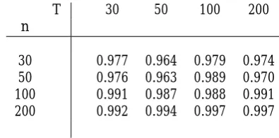
As far asf^tis concerned, we follow the same logic as in Bai (2). We compute the correlation coe¢ cient betweenff^tgTt=1andfftgTt=1, for each Monte Carlo iterationj- say

f

coe¢ cients, i.e. J 1PJ

j=1

f

j, in Table 1 (recall thatJ = 5000).

Table 1 illustrates that the estimated common factorf^tis highly correlated with the unobserved common factorft. This reinforces the results in Bai (2), albeit obtained in a di¤erent context, that the estimated factors are quite good at tracking the true ones; indeed, numerical values are very similar to those in Table 1 in Bai (2003, p.151). WhennandT are 100, the estimated factors can be treated as the true ones.

T 30 50 100 200

n

30 0.977 0.964 0.979 0.974 50 0.976 0.963 0.989 0.970 100 0.991 0.987 0.988 0.991 200 0.992 0.994 0.997 0.997

Table 1: Average correlation coe¢ cients betweenff^tgTt=1 andfftgTt=1.

As far as^_i is concerned, we report con…dence intervals for _i. In order to illustrate how con…dence intervals shrink asT expands, we setn= 50andT = 20;50;100;1000.

According to equation (6) in Theorem 1, as(n; T)! 1 with p

T

n !0, the95% con…dence interval forH 1 _i is given by^_i 1p:96

T

^1=2

i . Further, let^be the least square estimate of in = ^ +error, where = ( 1; : : : n)0 and ^ = (^1; :::;^n)0. The95% con…dence interval for i is therefore obtained as^ ^i 1p:96_T ^

1=2

i . By rotating^i towards i, we consider the con…dence interval for i directly, reported in Figure 1.

Figure 1: Con…dence intervals for _i. For each value of i = 1; :::;50 (on the horizontal axis), the solid line represents the true loading _i. The dashed lines are the con…dence intervals at95%con…dence level for each i.

Figure 1 shows that, in most cases and for all combinations of n and T, the con…dence intervals contain the true value of _i. This also holds true for the case(n; T) = (50;1000), where the ratio

p T n

is not negligible, as the theory would require. As predicted by the theory, as T grows, the con…dence intervals collapse to the true value of i.

4.2

Small sample properties -

S

and

S

Size Power

T T

n 30 50 100 200 30 50 100 200

2_{= 1=3} 2_{= 1=3}

30 0.077 0.066 0.060 0.056 0.950 0.996 1.000 1.000 50 0.073 0.063 0.050 0.056 0.986 0.999 1.000 1.000 100 0.073 0.063 0.052 0.045 0.997 1.000 1.000 1.000 200 0.072 0.062 0.053 0.042 0.998 1.000 1.000 1.000

2_{= 1=2} 2_{= 1=2}

30 0.086 0.074 0.064 0.059 0.867 0.968 0.999 1.000 50 0.078 0.067 0.053 0.058 0.926 0.993 1.000 1.000 100 0.074 0.063 0.053 0.046 0.972 1.000 1.000 1.000 200 0.073 0.064 0.054 0.042 0.992 1.000 1.000 1.000

2_{= 1} 2_{= 1}

30 0.109 0.094 0.081 0.076 0.612 0.800 0.976 0.999 50 0.090 0.079 0.065 0.068 0.667 0.883 0.993 1.000 100 0.085 0.070 0.058 0.051 0.764 0.952 1.000 1.000 200 0.076 0.067 0.057 0.044 0.863 0.983 1.000 1.000

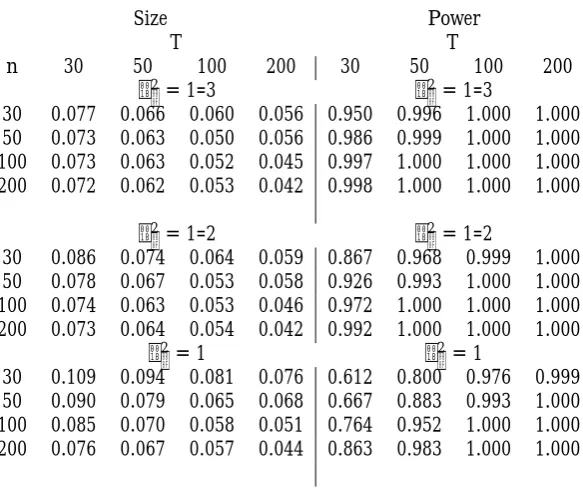
Table 2: Empirical rejection frequencies (for a nominal size of 5%) and power for tests forH₀a: i = , based on S ;nT. The DGP used in the simulations is (27)- (28).

As far as the design of the Monte Carlo is concerned, recall that the variance of the common compo-nentscit= iftis set equal to 1across all experiments. We conduct our simulations for di¤erent values of the signal-to-noise ratio V ar(cit)

2 , where

2 _{is the variance of it, equal to} 1 3;

1 2;1 .

Critical values have been computed by approximating Bn and BT as discussed in Section 3. Unre-ported simulations show that results worsen only slightly when using the asymptotic critical values.1

Testing for Ha

0 : i=

When evaluating the empirical rejection frequencies for tests based onS ;nT, we run the Monte Carlo simulations under the null _i= 1for alli. When evaluating power, we generate the loadings _i asi.i.d.

N 1; 2 , reporting results for the case of = 0:2. Given that itis cross sectionally uncorrelated and homoskedastic by design, iis estimated as ^ i= ^2 T F^0MxiF^

1

, where ^2= _nT1 Pn

i=1

PT

t=1^ 2

it. Results for size and power when using the main DGP (27)-(28) are in Table 2.

We …rstly consider the empirical rejection frequencies (left panel in the table). The test has a tendency to be oversized in small samples; as a general rule, the correct size is attained whenT 100andn 50; even when 2 _{= 1(low signal-to-noise ratio), the test has satisfactory size properties for T = 50. The}

Table also shows that, as the signal-to-noise ratio decreases (i.e., as 2 _{increases), the tendency towards}

Size Power

T T

n 30 50 100 200 30 50 100 200

2_{= 1=3} 2_{= 1=3}

30 0.044 0.037 0.037 0.030 0.915 0.959 0.988 0.996 50 0.038 0.034 0.036 0.033 0.993 0.999 1.000 1.000 100 0.042 0.041 0.036 0.032 1.000 1.000 1.000 1.000 200 0.046 0.043 0.038 0.036 1.000 1.000 1.000 1.000

2_{= 1=2} 2_{= 1=2}

30 0.047 0.036 0.037 0.030 0.773 0.860 0.935 0.970 50 0.040 0.035 0.036 0.033 0.957 0.987 0.998 1.000 100 0.042 0.042 0.037 0.033 0.999 1.000 1.000 1.000 200 0.047 0.044 0.038 0.037 1.000 1.000 1.000 1.000

2_{= 1} 2_{= 1}

30 0.054 0.042 0.038 0.032 0.467 0.525 0.635 0.733 50 0.047 0.038 0.039 0.035 0.703 0.822 0.912 0.962 100 0.049 0.047 0.038 0.035 0.967 0.994 0.999 1.000 200 0.055 0.050 0.041 0.040 1.000 1.000 1.000 1.000

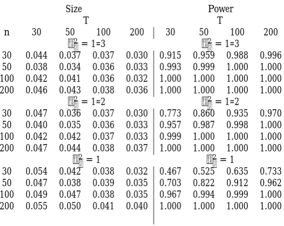
Table 3: Empirical rejection frequencies (for a nominal size of 5%) and power for tests forHb

0 :ft=f, based on Sf;nT. The DGP used in the simulations is (27)-(28).

small sample oversizement worsens. This is not so whenT 100andn 50: the test attains the correct size even for large values of 2_.

As far as the power is concerned (right panel in the Table), the test has good power properties in all cases: the power is above 50% for almost all cases. We note that, similarly to the size, the power deteriorates as the signal-to-noise ratio decreases; whennandT are su¢ ciently large, this disappears.

Testing for Hb

0 :ft=f

We run the Monte Carlo simulations under the nullft= 1for alltwhen evaluating the size of tests based on Sf;nT. When evaluating the power, we generate the common factors ft as i.i.d. N 1; 2f , reporting results for the case of f = 0:2. Finally, we estimate f t as f t = VnT1^

2 1

n

Pn

i=1^i^ 0 iV

1

nT

where ^2= 1

nT

Pn

i=1

PT

t=1^ 2

it.

Results when using (27)-(28) are shown in Table 3.

It can be noted that the test is slightly undersized for largeT, e.g. T 100. However, bothnandT

have a quite limited impact on the results. The test has very good power properties, especially when the signal-to-noise ratio is high. We note that the power increases with bothnandT, in a more pronounced way with n.

Size Power

T T

n 30 50 100 200 30 50 100 200

2_{= 1=3} 2_{= 1=3}

30 0.070 0.058 0.059 0.054 0.975 0.998 1.000 1.000 50 0.072 0.068 0.053 0.049 0.991 0.999 1.000 1.000 100 0.080 0.064 0.054 0.050 0.998 1.000 1.000 1.000 200 0.079 0.064 0.054 0.046 1.000 1.000 1.000 1.000

2_{= 1=2} 2_{= 1=2}

30 0.075 0.060 0.058 0.051 0.901 0.983 0.999 1.000 50 0.073 0.069 0.054 0.049 0.952 0.997 1.000 1.000 100 0.077 0.064 0.053 0.048 0.983 1.000 1.000 1.000 200 0.077 0.063 0.054 0.044 0.996 1.000 1.000 1.000

2_{= 1} 2_{= 1}

30 0.088 0.073 0.069 0.062 0.646 0.846 0.986 1.000 50 0.079 0.074 0.060 0.055 0.723 0.917 0.997 1.000 100 0.080 0.066 0.055 0.052 0.820 0.972 1.000 1.000 200 0.079 0.063 0.055 0.049 0.902 0.993 1.000 1.000

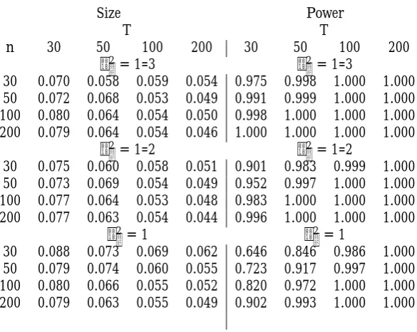
Table 4: Empirical rejection frequencies (for a nominal size of 5%) and power for tests forH₀a: _i = , based on S ;nT. The DGP used in the simulations is (27)- (28). The …rst-step estimator is the one proposed Song (33).

(27)-(28), show that the test procedure is una¤ected by the choice of the …rst step estimator when this is a consistent one. Finally, we point out that in Castagnetti, Rossi and Trapani (2014), we provide further Monte Carlo evidence based on alternative DGPs. The Monte Carlo results con…rm for both tests good properties in terms of size and power.

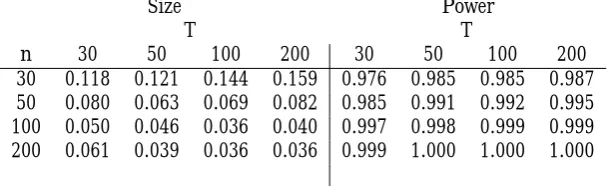
Autocorrelated and heteroskedastic idiosyncratic errors

In order to assess the …nite sample properties of the two test procedures when the errors are autocor-related and heteroskedastic, we consider the following DGP:

it= 0:5 it 1+uit

uit IIDN(0; 2ui)

2

ui U(0:1;0:5)

and we make use of the HAC estimators for and f given by equations (7) and (10). Apart from these features, the experiments have the same speci…cations as above, with V ar( it)2(0:13;0:67).

undistinguishable from the ones computed with i.i.d. errors. As far as, the power is concerned, both tests have good properties and are very close to thei.i.d. case.

Size Power

T T

n 30 50 100 200 30 50 100 200

30 0.103 0.087 0.088 0.100 0.838 0.905 0.966 0.994 50 0.090 0.083 0.078 0.074 0.956 0.988 0.999 1.000 100 0.081 0.071 0.063 0.065 0.999 1.000 1.000 1.000 200 0.072 0.061 0.063 0.054 1.000 1.000 1.000 1.000

Table 5: Empirical rejection frequencies (for a nominal size of5%) and power for tests for Hb

0 : i= . The test is computed using the estimator of i in (7).

Size Power

T T

n 30 50 100 200 30 50 100 200

30 0.118 0.121 0.144 0.159 0.976 0.985 0.985 0.987 50 0.080 0.063 0.069 0.082 0.985 0.991 0.992 0.995 100 0.050 0.046 0.036 0.040 0.997 0.998 0.999 0.999 200 0.061 0.039 0.036 0.036 0.999 1.000 1.000 1.000

Table 6: Empirical rejection frequencies (for a nominal size of 5%) and power for tests forHb

0 :ft=f. The test is computed using the estimator of f tin (10).

5

Conclusions

In this contribution, we develop an inferential theory for the unobservable common factors and their loadings in a large, stationary panel model with observable regressors. Our framework allows for slope heterogeneity; we also allow for correlation between common factors and observable regressors, by mod-elling the DGP of the observable regressors as containing the common factors, in a similar spirit as in Pesaran (30).

or unit speci…c) common e¤ects, so that common features in the panel can be captured by inserting time dummies or unit speci…c dummies. The proposed test procedures simplify the speci…cation analysis of heterogeneous panel data models with unobserved factors. From a methodological perspective, this entails that the tests can be implemented without prior knowledge of the number of factors. The only thing which is needed is a consistent preliminary estimation of the slope parameters. Building on this, we propose statistics based on extrema of the estimated loadings and common factors. Under the null, the test statistics converge to an Extreme Value distribution. As far as power is concerned, from a theoretical point of view our tests are consistent even under alternatives where only one loading or common factor di¤ers from the average. Monte Carlo evidence shows that both tests have the correct size and good power properties.

Building on the theory developed in this paper, there are several interesting avenues for further developments. An important case is the estimator of the _is used in Step 1. In our paper, we focus on the CCE estimator proposed by Pesaran (30); this estimator is easy to treat analytically, but it is only a possible choice. In particular, our setup requires strict exogeneity, thereby ruling out e.g. the possibility of having lagged values of theyits among the regressors. This requirement is due to the estimation method employed in Step 1, rather than to the inference on factors and loadings per se. Indeed, the CCE is known not to work in presence of weakly exogenous regressors (see 20; and 12). However, the assumption of strict exogeneity can be readily relaxed (accommodating e.g. for dynamic models), upon employing, in Step 1, an estimator of the _is that is consistent at a rateOp min T 1=2; n 1 . A possible choice for this case is the IE estimator studied in Song (33), which has the desired convergence rate, even in presence of dynamic models. Alternatively, a di¤erent approach, based on unit speci…c estimators can be used, by instrumenting the unobservable common factors ft using the regressors xjt for each uniti, with i6=j - indeed, both the CCE and the IE have a natural Instrumental Variable interpretation (see also 4). Such extensions are currently under investigation of the authors.

Acknowledgement

Appendix: technical results and proofs

In this section we set the rotation matrixH =Ir whenever possible in order to simplify the notation. The proofs of the Lemmas, and the proof of Theorem 4, are given in Castagnetti, Rossi and Trapani (10).

Lemma A.1Under Assumptions 1-4, it holds that, for every i, E ~_{i i}

r

= O _nTr , for any

r 3.

Lemma A.2Under Assumptions 1-4, it holds that, for every i

A.2(i) T 1 0

i F^ F =Op nT2 ;

A.2(ii) n 1=2T 1Pn

i=1 0i F^ F =Op n 1=2 +Op T 1 .

Lemma A.3. It holds that, for every i

A.3(i) T 1_X0

i F^ F H =Op nT2 ;

A.3(ii) T 1F0 F^ F H =Op nT2 ;

A.3(iii) T 1 _F^ _{F H} 0 _F^ _{F H =O}

p nT2 .

Lemma A.4 Let Assumptions 1-4 hold. Under H0a that i = , it holds that b =Op nT2 as (n; T)! 1.

Lemma A.5 Let Assumptions 1-4 hold. Under H₀b that ft =f, it holds that bf f =O_{p nT}2 as

(n; T)! 1.

Lemma A.6Let Assumptions 1-4 hold, and let kdenote the largest …nite moment of it,ftand xit.

It holds that

A.6(i) max1 i n ~i i

2

=op n2=k nT2 ;

A.6(ii) max1 t T f^t H0ft

2

=op T2=k nT2 ;

A.6(iii) max1 i n ^i H 1 i

2

=op n2=kT 1 +op n2=k 2T ;

A.6(iv) max1 t T^2it=op T2=k +op T2=k nT2 ;

A.6(vi) max1 i n^2it=op n2=k +op n4=k nT2 +op n2=k 2T ;

A.6(vii) max1 i n ^2it 2it =op n4=k nT2 +op n2=k 2T .

Lemma A.7Let Assumptions 1-4 hold, and let kdenote the largest …nite moment of it,ftand xit:

A.7(i) if, in addition, Assumption 6 holds, then T 1_F^0_{F^ H}

fH0 =Op T 1=2 +Op n 1 ;

A.7(ii) if, in addition, Assumption 6 holds, then max1 i n T 1F^0MXiF^ f M;i = Op T 1=2 +

Op n 1 ;

A.7(iii) if, in addition, Assumption 8 holds, thenmax1 t T ^ ;t H 1 ;t H 1

0

=op T2=k nT1 ;

A.7(iv) if, in addition, Assumption 8 holds, then max1 i n ^ ;i ;i =op

p

T n2=k 2

nT ;

A.7(v) if, in addition, Assumption 6 holds, then max1 i n T 1=2F0MXi i Ni =op n1=kT1=k 1=2 ,

where fNig n

i=1 is a sequence of i.i.d. Gaussian random variables, with variances f M e;i;

A.7(vi) if, in addition, Assumption 8 holds, thenmax1 t T n 1=2P n

i=1^i it Nt =op T1=kn1=k 1=2 +op T1=k nT1 +op T1=k

p

n _nT2 , where fNtg T

t=1 is a sequence of i.i.d. Gaussian random vari-ables, with variances ;t.

Proof of Theorem 1. By de…nition, we have

p

T(^_{i i}) = ^

F0MXiF^

T

! 12 4

^

F0MXi i

p T

^

F0_M

Xi F^ F i

p T

3

5: (29)

We start by considering the denominator of (29):

^

F0_M XiF^

T

F0_M XiF

T

=

F0MXi F^ F

T +

^

F F

0

MXiF

T

^

F F

0

MXi F^ F

T =I+I

0 _II:

Repeated application of Lemma A.3 yields I = Op nT2 and II = Op nT4 . Thus, as (n; T) ! 1,

T 1_F^0_M

XiF^ =T 1F0MXiF+op(1).

We turn to the numerator of (29). It holds that

^

F0MXi i

p

T =

F0MXi i

p

T +

^

F F

0

MXi i

p

By applying a similar logic as in the proof of Lemma A.4, it can be shown that I=Op(1). As far asII is concerned, note

II = p T ^ F F 0 i T + ^ F F 0 Xi T X0 iXi

T 1 X0 i i p T ;

applying Lemma A.2(i) (to the …rst term), and Lemma A.3(i) and Assumptions 2(i) and 1(i) (to the second term), it follows thatII =Op

p

T _nT2 . Thus, the numerator of (29) is of orderOp(1)+Op p

T n . Finally, as(n; T)! 1under the restriction

p T

n !0, (29) becomes

p

T(^_{i i}) = F 0_M

XiF

T

1

F0MXi i

p

T +op(1) ;

equation (6) follows from Assumption 5(i). QED

Proof of Theorem 2. Using (1) in Castagnetti, Rossi and Trapani (2014), we can write

^

ft ft = 1 n n X j=1 ^

F0Xj

T

!

~

j j ~j j 0

xjt (30)

1

n

^

F0F T

! n

X

j=1

j ~j j 0 xjt 1 nT n X j=1 ^

F0 j ~j j 0 xjt 1 n n X j=1 ^

F0Xj

T

!

~ j j

0 jft

1 n n X j=1 ^

F0Xj

T

!

~

j j jt

+ 1 nT n X j=1 ^

F0 j 0jft+ 1

n

^

F0F T

! _n X

j=1

j jt+ 1 nT n X j=1 ^

F0 j jt

= I II III IV V +V I+V II+V III:

The order of magnitude ofIfollows exactly from the same passages as in the proof of Lemma A.5, with

I=Op nT2 . ConsiderII; omitting j in view of Assumption 3(iii), we have

II= 1

n

^

F0_F

T

! n

X

j=1

0 jxjt+

1

n

^

F0_F

T

! n

X

j=1

0

jxjt=IIa+IIb;

we have shown that IIa = Op n 1=2T 1=2 and IIb = Op n 1=2T 1=2 + Op n 1 in the proof of Lemma A.3, so that II = Op n 1=2T 1=2 +Op n 1 . Using Lemma A.3(i), it can be shown that

III =Op nT2 . As far asIV is concerned, note that

IV = ^ F0 p T 1

npT

n

X

j=1

Xj j 0jft+ 1 n n X j=1 ^

F0Xj

T

!

Similar passages as in the proof of the order of magnitude of IIa, and the fact that Ekftk M entail

IVa = Op n 1=2T 1=2 . Similarly, IVb is bounded by kftk E

^

F0Xj

T

2 1=2 h

E j

2i1=2

, which is

Op n 1=2 nT1 using Lemma A.1. Thus,IV =Op n 1=2 nT1 . Turning toV, we have

V = 1

n

n

X

j=1

^

F0Xj

T

!

~

j j jt

= 1 n n X j=1 ^

F0Xj

T

!

X_j0MwXj

T

! 1

X_j0Mw j

T ! jt +1 n n X j=1 ^

F0Xj

T

!

X_j0MwXj

T

! 1

X_j0MwF

T j

!

jt=Va+Vb:

We start from Vb n 1 P n j=1

^

F0_X

j

T

X0_jMwXj

T

1 _X0

jMwF

T j j jtj. Using Assumptions 3(iii) and 4(i), Vb is bounded by E

h _F^0_X

j

T

X_j0MwF

T j jtj

i

E F^

0_X

j

T

6 1=6

E X

0

jMwF

T

3=2 2=3

Ej jtj

6 1=6

= O n 1 + O n 1=2T 1=2 , where the passage in the middle follows from Holder’s in-equality. Consider nowVa:

Va = 1

n

n

X

j=1

F0Xj

T

X_j0MwXj

T

! 1

X_j0Mw j

T ! jt +1 n n X j=1 ^

F F 0Xj

T

X_j0MwXj

T

! 1

X_j0Mw j

T

!

jt=Va;1+Va;2:

Consider Va;2:

Va;2

1 n n X j=1 ^ F F 0 Xj T

X_j0MwXj

T

! 1

X_j0Mw j

T j jtj

M1 n n X j=1 ^ F F 0 Xj T

X_j0Mw j

T j jtj;

using Assumption 4(i). Further,E (F^ F)

0 Xj

T

X_j0Mw j

T j jtj E

(F^ F)0 Xj

T

3=2!2=3

E X

0

jMw j

T

6 1=6

Ej jtj

6 1=6

Va;2=Op T 1=2 nT2 . Turning toVa;1

Va;1 =

1

n

n

X

j=1

F0Xj

T

X0 jMwXj

T

! 1

X0

jMwE(j jt)

T +1 n n X j=1

F0_X j

T

X_j0MwXj

T

! 1

X_j0Mw[ j jt E( j jt)]

T =Va;1;1+Va;1;2:

By virtue of Assumption 4(i),Va;1;1 M n 1T 2P

n

j=1kF0Xjk Xj0MwE( j jt) . We haveE

h _F0_X

j

T

X_j0MwE(j jt)

T

i

E F0Xj

T

2 1=2

E X

0

jMwE(j jt)

T

2 1=2

, withE F0Xj

T

2

M by Assumption 2(i). Further,

E X

0

jMwE( j jt)

T 2 1 T2 T X s=1 T X u=1

E[kxjsk kxjuk]E( js jt)E( ju jt)

M 1 T2

" T

X

s=1

E(js jt)

#2

=O 1 T2 ;

where we have used Assumptions 4(i), 2(i) and 1(ii)(a). Consider now Va;1;2; this is bounded by the

square root of

E 8 < : 1 n2 n X j=1 n X k=1

F0Xj

T

F0Xk

T

X_j0MwXj

T

! 1

X_k0MwXk

T

1

X_j0Mw[ j jt E(j jt)]

T

X_k0Mw[ k kt E( k kt)]

T

)

;

after some algebra, this is bounded by

E

8 <

:

1

n2_T2

n X j=1 n X k=1

F0Xj

T

F0Xk

T T X s=1 T X u=1

xjsxku[ js jt E( js jt)] [ju jt E( ju jt)]

9 =

;

= 1

n2_T2

n X j=1 n X k=1 T X s=1 T X u=1 E F 0_X j T

F0Xk

T xjsxku Ef[ js jt E( js jt)] [ ju jt E( ju jt)]g

1

n2_T2

n X j=1 n X k=1 T X s=1 T X u=1

Ef[ js jt E( js jt)] [ ju jt E( ju jt)]g

1 nTE 1 p nT n X j=1 T X s=1

[ js jt E( js jt)]

2

;

+Op n 1=2T 1=2 . The proofs ofV I=Op n 1=2T 1=2 ,V II =Op n 1=2 andV III =Op nT2 are based on the same arguments as in Bai (2), since the estimation error ~_{j j} does not appear in their expression. Putting everything together, as(n; T)! 1with

p n

T !0, the term that dominates in the

expansion of f^t ft is V II, whose asymptotics is exactly the same as studied in Bai (2, Theorem 1). QED

Proof of Theorem 3. Prior to proving the Theorem, we lay out some preliminary results and notation. We write

^i b= ( i ) + (^i i) b =ai+bi ci:

Under Ha

0, ai = 0; also,bican be rewritten asbi = ^i . Using (29), we have

bi = F^0MXiF^

1

F0MXi i+ F^0MXiF^

1

^

F F

0

MXi i (31)

^

F0MXiF^

1

^

F0MXi F^ F i

= b1i+b2i;

where we de…neb1i= F^0MXiF^

1

F0MXi iandb2iis the remainder. Further, we can write ^ i1=

1

i

1

i ^ i i i1 +op ^ i i for each i. Neglecting higher order terms that depend on

op ^ i i , we have

T ^_i b

0_{^ 1}

i ^i b (32)

= T b0_{1i i}1b1i +T b01i

1

i ^ i i i1b1i+T b02i^

1

ib2i +2T b01i^

1

ib2i+T b

0 _^ 1

i b 2T b

0_^ 1

i (^i )

= T b0_{1i i}1b1i +Ii+IIi+IIIi+IVi Vi:

After this preliminary calculations, we turn to proving (20). In order to do this, we …rstly show that max1 i nT b01i

1

ib1i can be approximated by the maximum of a sequence of independent random variables with a 2r distribution, up to a negligible error. Given that the maximum of a sequence of chi-squares is of orderOp(lnn), the approximation error should beop(lnn)at most. Secondly, we show that Ii Vi in (32) are also allop(lnn)uniformly ini.

Considermax1 i nT b01i

1

ib1i , and consider in particular the sequence

np

T b1i

on

i=1

. It holds that

p T b1i=

h

T 1F^0MXiF^

i 1

T 1=2F0MXi i . As far as the numerator of this expression is concerned, by Lemma A.7(v) we writeT 1=2_F0_M

Gaussian with covariance matrix f M e;i, andRN i =op n1=k1T1=k1 1=2 . As far as the denominator of

p

T b1iis concerned, based on Lemma A.7(ii)we write

h

T 1_F^0_M XiF^

i 1

= _{f M;i}1 +R f M;iwithR f M;i =Op T 1=2 +Op n 1 . Hence we write

p T b1i=

h

1

f M;i+R f M;i

i

[Ni+RN i]: (33)

Based on (33), and on the de…nitions of f M e;i and of f M;i, it holds that

T b01i

1

ib1i = Ni0

1

f M e;iNi+ 2Ni0

1

f M;i

1

i RN i+ 2R0N i

1

f M e;iNi (34) +2N_i0 _{f M;i}1 _i1R f M;iNi+ 2Ni0

1

f M;i

1

iR f M;iRN i

+R0_{N i f M e;i}1 RN i+ 2R0N i

1

f M;i

1

iR f M;iRN i

+N_i0R f M;i i1R f M;iNi+ 2Ni0R f M;i i1R f M;iRN i +R0_{N i}R f M;i i1R f M;iRN i

= N_i0 _{f M e;i}1 Ni+Iib1+II b1

i +III b1

i +IV b1

i +V b1

i +V I b1

i

+V II_ib1+V III_ib1+IX_ib1:

We note that the distribution ofN_i0 _{f M e;i}1 Niis 2r. We now show that, in (34),max1 i nIib1; :::;max1 i nIXib1 are allop(1). Considermax1 i nIib1; this is bounded bymax1 i nkNikmax1 i nkRN ik=op n1=k1T1=k1 1=2

p

lnn , in view of Lemma A.7(v)and the fact thatmax1 i nkNik=Op

p

lnn . The same holds formax1 i nIIib1. Turning to max1 i nIIIib1, it is bounded by max1 i nkNik

2

max1 i nkR f M;ik = Op T 1=2lnn + Op n 1lnn by virtue of Lemma A.7(ii). As far as max1 i nIVib1 is concerned, it is bounded by max1 i nkNik max1 i nkR f M;ik max1 i nkRN ik, and therefore it is dominated by the previ-ously analyzed terms. Also, max1 i nVib1 has the same order of magnitude as max1 i nkRN ik2, thereby being dominated by the other terms. Similarly,max1 i nV Iib1is bounded bymax1 i nkRN ik2 max1 i nkR f M;ik, and therefore it is also dominated. Turning to max1 i nV IIib1, it is bounded by max1 i nkNik

2

max1 i nkR f M;ik

2

, so that it is smaller thanmax1 i nIIIib1, and therefore negligi-ble. Similarly, max1 i nV IIIib1 is bounded bymax1 i nkNik max1 i nkR f M;ik

2

max1 i nkRN ik, which is dominated by max1 i nIVib1, and thus negligible. Finally, max1 i nIXib1 is bounded by max1 i nkR f M;ik

2

max1 i nkRN ik

2

, and it is dominated. Therefore

max

1 i nT b 0

1i

1

ib1i = max

1 i nN 0 i

1

f M e;iNi+op

"

(nT)1=k1

r

lnn T

#

+Op lnn p

T +Op

lnn

After proving thatmax1 i nT b01i

1

i b1i can be approximated bymax1 i nNi0

1

f M e;iNi, we turn again to equation (32). We now show thatmax1 i nIi,:::,max1 i nVi are allop(lnn). ConsiderIi; it holds that

max

1 i nIi 1maxi nT b 0

1i

1

ib1i max

1 i n

1

i ^ i i i1 : Equation (35) implies thatmax1 i nT b01i

1

ib1i =Op(lnn); thus, applying Lemma A.7(iv),max1 i nIi =op

p

T n2=k1 2

nTlnn . Turning tomax1 i nIIi, note that, in equation (31),b2i is de…ned as

b2i= F^0MXiF^

1

^

F F

0

MXi i F^0MXiF^

1

^

F0MXi F^ F i;

further, by the invertibility of _i1 and Lemma A.7(iv), max1 i nT b02i^

1

ib2i has the same or-der of magnitude as max1 i n

p T b2i

2

max1 i n i1 ^ i i i1 . Considering max1 i n

p T b2i

2

, it can be evaluated by considering the orders of magnitude ofmax1 i n

p

T F^0MXiF^

1

^

F F

0

MXi i

2

and of max1 i n

p

T F^0MXiF^

1

^

F0MXi F^ F i

2

. The former can be shown to be op n2=k1T nT4 , based on the proof of Lemma A.6(iii). The latter has the same order of magnitude as T 1=2_F^0 _F^ _F 2_{, which is Op T} 4

nT by Lemma A.3(iii). Putting all together, max1 i nIIi = op T3=2n4=k1 nT6 - so, max1 i nIIi is dominated by max1 i nIi. Similar passages yield that max1 i nIIIi is dominated bymax1 i nIIi. Turning to IVi, it holds that max1 i nIVi

p T b

2

max1 i n i1 ^ i i i1 , which isop T n2=k1 nT6 by Lemmas A.4 and A.7(iv). Finally,max1 i nViis bounded by

p

T b max1 i n

p

T b1i max1 i n i1 ^ i i i1 =op T n2=k1 nT4lnn . Putting all together, and using (35), it holds that

max

1 i nT ^i b 0 _^ 1

i ^i b = max

1 i nN 0 i

1

f M e;iNi+op

"

(nT)1=k1

r

lnn T

#

(36)

+op

n2=k1

p

T lnn +op p

T n2=k1

n lnn

!

+op(1);

where the remainders are negligible as(n; T)! 1with (nTp)1=k1 T +

p T n2=k1

n !0 and n4=k1

T !0, which

hold in light of (19). Finally, consider the sequencefNig n

i=1: the covariance between

p

T b1i and

p T b1j is given by

E F

0_M

Xi i 0jMXjF

T E

F0 i 0jF

T = 1 T T X t=1 T X s=1

E(ftfs it js0 )

1 T T X t=1 T X s=1

kE(ftfs0)k jE(it js)j M 1 T T X t=1 T X s=1

which tends to zero as (n; T) ! 1 by Assumption 7. By virtue of the asymptotic independence be-tween Ni and Nj for all i =6 j, the asymptotics ofmax1 i nNi0

1

f M e;iNi is studied e.g. in Embrechts, Klüppelberg and Mikosch (1997, Table 3.4.4, p.156). Thus, equation (20) follows from (36).

We now …nish the proof of the Theorem, analysing the power properties of the test. In order to evaluate the presence of power when _i6= for some (at least one)i, after some algebra it can be shown that, under the alternative,S ;nT has non-centrality parameter given by

SN C;nT =T max

1 i nc 0 i^

1

ici+ 2T max

1 i nc 0 i^

1

i (^i i) 2T max

1 i nc 0 i^

1

i b =I+II III;

withI=Op Tkcik

2

by construction. Also,II is bounded by

p

T(max1 i nkcik) max1 i n

p

Tk^_{i i}k =Op T nT2n1=k1kcik in view of Lemma A.6(iii); simi-larly, III=Op

p

T _nT2kcik by Lemma A.4. LetS_nT;0denote the null distribution of S_nT; underH1a it

holds that

P[S ;nT > c ;n] =P

h

S_nT;0> c ;n SnT;N C

i

;

which tends to 1 if c ;n SN C;nT ! 1 as (n; T) ! 1. In view of equation (22), we know that

References

[1]

[2] Bai, J., 2003, Inferential theory for structural models of large dimensions. Econometrica, vol. 71, 135-171.

[3] Bai, J., 2009a, Panel data models with interactive …xed e¤ects. Econometrica, vol. 77, 1229-1279.

[4] Bai, J., 2009b, Supplement to Panel data models with in-teractive …xed e¤ects : technical details and proofs. Econo-metrica, vol. 77, 1-30.

[5] Baltagi, B., Kao, C., Na, S., 2012, Testing cross-sectional dependence in panel factor model using the wild bootstrap F-test, manuscript.

[6] Bai, J., Ng, S., 2002, Determining the number of factors in approximate factor models. Econometrica, vol. 70, 191-221.

[7] Berman, S.M., 1964, Limit theorems for the maximum term in stationary sequences. The Annals of Mathemat-ical Statistics , vol. 35, 502-516.

[8] Canto e Castro L., 1987, Uniform rate of convergence in extreme-value theory: normal and gamma models. An-nales Scienti…ques de l’Université de Clerment-Ferrand, 2, tome 90, Série Probabilités et Applications, vol. 6, 25-41.

[9] Castagnetti, C., Rossi, E., Trapani L., 2014a, Supple-ment to ”Inference on Factor Structures in Heterogeneous Panels”. Technical details, proofs and further simulations. Mimeo, June 2014.

[11] Castagnetti, C., Rossi, E., 2013, Euro corporate bond risk factors. Journal of Applied Econometrics, vol. 28, 372-391.

[12] Chudik, A., Pesaran, H., 2013, Common Correlated E¤ects Estimation of Heterogenous Dynamic Panel Data Models with Weakly Exogenous Regressors. CESifo Working Pa-per Series 4232.

[13] Chudik, A., Pesaran, H., Tosetti, E., 2011, Weak and strong cross-section dependence and estimation of large panels. Econometrics Journal, vol. 14, 45-90.

[14] Corradi, V., 1999, Deciding between I(0) and I(1) via ‡il-based bounds. Econometric Theory, vol. 15, 643-63.

[15] Csörgö, M., Hórvath, L., 1997, Limit theorems in change-point analysis. Wiley, Chichester.

[16] Eberhardt, M., Helmers, C., Strauss, H., 2013, Do spillovers matter when estimating private returns to R&D?. The Review of Economics and Statistics, vol. 95, 436-448.

[17] Eberhardt, M., Teal, F., 2012, No mangos in the tundra: spatial heterogeneity in agricultural productivity analysis. Oxford Bulletin of Economics and Statistics (forthcoming).

[18] Eberlein, E., 1986, On strong invariance principles under dependence assumptions. Annals of Probability, vol. 14, 260-270.

[19] Embrechts, P., Klüppelberg, C., Mikosch, T., 1997, Mod-elling extremal events for insurance and …nance. New York: Springer.

[21] French, D., O’Hare, C., 2013, A dynamic factor approach to mortality modeling. Journal of Forecasting (forthcom-ing).

[22] Hall, P., Miller, H., 2010, Bootstrap con…dence inter-vals and hypothesis tests for extrema of parameters. Bio-metrika, vol. 97, 881-892.

[23] Hannan, E.T., Kavalieris, L., 1986. Regression; autoregres-sion models. Journal of Time Series Analysis, vol. 7, 27-49.

[24] Jenish, N., Prucha, I.R., 2012. On spatial processes and as-ymptotic inference under Near-Epoch Dependence. Jour-nal of Econometrics, vol. 170, 178-190.

[25] Kapetanios, G., 2003, Determining the poolability of indi-vidual series in panel datasets. University of London Queen Mary Economics Working Paper No. 499.

[26] Kapetanios, G., Pesaran, M.H., 2007, Alternative ap-proaches to estimation and inference in large multifactor panels: small sample results with an application to mod-elling of asset returns. In Garry Phillips and Elias Tzavalis, (Eds.), The Re…nenement of Econometric Estimation and Test Procedures: Finite Sample and Asymptotic Analysis. Cambridge University Press, Cambridge.

[27] Leadbetter, M.R., Rootzen, H., 1988, Extremal theory for stochastic processes. Annals of Probability, vol. 16, 431-478.

[28] Lee, R. D., Carter, L. R., 1992, Modeling and forecasting the time series of U.S. mortality. Journal of the American Statistical Association, vol. 87, 659-671.

[30] Pesaran, M. H., 2006, Estimation and inference in large heterogeneous panels with a multifactor error structure. Econometrica, vol. 74, 967-1012.

[31] Pesaran, M. H., Tosetti, E., 2011, Large panels with com-mon factors and spatial correlation. Journal of Economet-rics, vol. 161, 182-202.

[32] Sara…dis, V., Yamagata, T., Robertson, D., 2009, A test of cross section dependence for a linear dynamic panel model with regressors. Journal of Econometrics, vol. 148, 149-461.

[33] Song, M., 2013. Asymptotic theory for dynamic heteroge-neous panels with cross-sectional dependence and its ap-plications. Mimeo, January 2013.