Nonlinear Aircraft Engine Model for Future Integrated Power Center Development
Hossein Balaghi Enalou, Mohamed Rashed, Ponggorn Kulsangcharoen, Christopher Ian Hill, Serhiy Bozhko
Department of Electrical and Electronic Engineering, Faculty of Engineering,University of Nottingham, University Park, Nottingham, UK, NG7 2RD. Email: [email protected]
Abstract—Aircraft engines, the prime source of on-board
power, play a vital role within the electrical power generation system. In literature these are considerably simplified to rudimentary engine speed. In this paper, a nonlinear zero-dimension (0-D) order turbofan engine model has been developed for use with an integrated power center. By analyzing the compressor maps in detail, the results reveal a limit on the amount power off-take from each engine shaft at different altitudes.
Keywords—Turbofan, Modeling, power off-take
I. INTRODUCTION
A lot of research has been done on modelling of aircraft electrical generation systems for which the only input is the mechanical speed of the aircraft engine. Within these systems the AC power frequency is variable and depends of the engine speed. The interface between the engine and aircraft is therefore considerably simplified, having been reduced to electric power, fuel and control signals only. This inflexibility prevents further analysis of the integrated power center as detailed consideration of the prime source of on-board power is not included.
For this purpose, the first step is to develop an accurate model of the aircraft engine with an adequate degree of accuracy and complexity. Almost all modern aircraft engines are designed as multiple spool turbofans with high-bypass ratios to minimize fuel consumption and reduce generated noise. Single shaft engines can be modelled as a linear system [2], however, nonlinear modelling is required for multiple spool gas turbines due to the thermodynamic coupling between compressor-turbine sets.
Depending on the application of model, it can be 0-order, 1st order, 2ndorder or 3rdorder. It is generally accepted that a 0-D simulation is sufficient for accurate dynamic performance modeling and therefore controller design [3]. For this purpose, there are two main approaches; the iterative approach and the inter component volume method.
In the iterative approach [4]-[6], mainly used by the Controls and Dynamics Branch of NASA, the number of state variables is equal to the number of shaft inertias. Using this approach, all other performance data are calculated through thermodynamic laws as well as an iterative solver to reduce the flow continuity errors between components.
The Inter Component Volume method (ICV) on the other hand is quite simple and faster for transient simulation. In reality, components have their own physical gas storage volumes that cause a lag in flow transfer within them [4]-[8].
[image:1.596.339.532.233.390.2]In the developed model, power can be generated from both the High Pressure (HP) and Low Pressure (LP) engine shafts. Moreover, the model provides the capability of exchanging power between the HP and LP shafts through starter-generator electrical machines as shown in Fig. 1. In this way, the engine interactions and control of Electric Power System (EPS) energy storage integration and optimized operation depending on Engine Operating Mode (EOM) can be studied.
Fig. 1. Off-take power from the jet-engine
II. ENGINE MODELING
The ICV method was implemented in the
MATLAB/SIMULINK [9] environment. Using this approach, the major engine components included in the model (see Fig. 2) are: inlet duct, fan (modelled as separate duct and core sections), bypass duct, booster (Low Pressure Compressor (LPC)), inter-compressor bleeds, High Pressure Compressor (HPC) and cooling bleeds, fuel metering valve and fuel manifold, combustion chamber, High Pressure Turbine (HPT) with cooling, Low Pressure Turbine (LPT) and discharge nozzles.
[image:1.596.336.539.549.682.2]Fig. 3 and Fig. 4 illustrate the arrangement of the engine component where ?̇, T, Pand ωare mass flow, temperature, pressure and rotor speed respectively.
Fig. 3. Illustration of Jet-engine component models integration
Fig. 4. Equivalent electrical circuit analogy of the Jet-engine component modelling
It should be noted that all variants of this model are in the International Systems of Units (SI). Within each component, the inputs are inlet and outlet pressure, temperature and shaft speed. This data is then used to find the performance point of each respective component. Components are represented by maps in which corrected mass flow and adiabatic efficiency are indexed by corrected shaft speed and pressure ratio (see Fig. 5). More information about corrected speed, mass flow and how to use maps is well documented in [11]. It is important to maintain mass/momentum/energy balance through each component. Having inlet mass flow and efficiency, and by implementing thermodynamic laws for open systems, outlet temperature and power can be obtained. Once mass flow and efficiency of every component has been interpolated using component maps, outlet temperature is calculated using (1) and (2):
for compressors:
????? ????? ???
??? ?
??
?
−
???(1)
for turbines:
????? ????? ? ????
? ??
?
−
???(2)
where ?? and ??are compressor and turbine efficiencies and
?is pressure ratio of the component ?????? ??
? ?. ?and ??are
from thermodynamic tables for the mean temperature of inlet and outlet flow [12]. The required power to drive the compressor, PShaft, or the generated power produced by turbine
can also be calculated as:
??????? ?̇??????
−
?????(3)
In the Control Volume (CV) subsystem shown in Fig. 5, a volume is assumed to be an open thermodynamic system in which thermodynamic laws are applied to calculate state variables. Within the CV subsystem considered here, the state variables are pressure and temperature as shown in Fig. 5. No work is done on fluid in CV analysis and heat transfer is assumed to be zero in this model. ????and ????are assumed
to be equal to Tand pwhen applying CV analysis. The change in mass inside the CV is calculated using:
????
?? ? ?̇??
−
?̇???(4)
where ??? is the current mass of the CV. Pressure,
Temperature and volume of the mass inside the CV are related by using the ideal gas law as below:
?? ? ?????
(5)
where V is volume of the CV and R is the specific gas constant. Pressures and temperatures are total amounts including the effect of the gas speed impact. By using (4) and (5), the outlet pressure can be determined as shown in Fig. 6.
Control Volume Component Control Volume
From next component Power
To shaft inertia module
in
T Tin
in P
in T
out P
From shaft inertia module
[image:2.596.44.282.94.285.2]w
Fig. 5. Structure of gas turbine model
LP
C HPC Combustor HPT LPT
Pi,T
i
PLPC ,TLP
C
PHPC ,THPC
PCB ,TCB
PHPT ,THPT
PHPT ,THPT
Fuel Metering unit
m
f
mHPC
mLPC mHPT mLPT
FA
N P
FA
N
,TFA
N
mFAN bym
pa
ss
Ti, Pi mLPC PLPC mHPC PHPC PCB mHPT
m
f
PHPT
∑use PR and N to determine m and h.
from the maps.
∑use gas properties to calculate: T and h.
∑use h and h. to calculate torque.
V/(RTLPC) V/(RTHPC) V/(RTHPT)
PFAN
mFAN
V/(RTFAN)
m
by
pa
[image:2.596.133.467.519.637.2]1 s
V R
-+
in
m&
out
m&
out
P
¥
in
T
P C
¥
P C
f
m& LHV
+
+- s1
¥
∏
∏
v C
out
T
[image:3.596.51.272.51.231.2]¥
Fig. 6. Control volume module
The change in internal energy of control volume?̇ can also be calculated as:
?̇ ? ???
−
????(6)
where ? and ? are internal energy of the control volume and flow enthalpy respectively. ?and ?are calculated as follows:
? ? ??????
(7)
? ? ?̇???
(8)
where ?? and ?? are specific heat at constant volume and pressure respectively. The energy released by fuel burning is obtained by the equation below:
??? ?̇????
(9)
where ?̇? is fuel mass flow and ??? is the Lower Heating
Value of fuel. Using equations (6)-(9) the block for outlet temperature is shown in Fig. 6. ?̇? is zero for all control
volumes except for the control volume within combustion chamber.
The engine model presented in this paper is based on physical rules, however during the modelling process assumptions and simplifications have to be made, thus deviations from reality are expected. For this reason, the main parameters of the model are calibrated at the design condition of the engine. As the model is modular it can be easily modified for other multiple spool turbines by simply swapping component maps, shaft inertias and LHVfor fuel.
The torque generated by the HPT and LPT are required to drive HPC and LPC+FAN through the HP and LP shafts respectively. Both shafts also drive independent starter-generator machines when in starter-generator mode. Fig. 7 shows the torques which are imposed on the rotor by the turbine (TGT)
and the compressor or generator (TLoad).
Fig. 7. Solid rotor
If the turbine rotor is assumed to be solid, Newton’s second law gives:
???
−
? ? ??̇(10)
where Jis the rotor moment of inertia and ωis the shaft speed. The relation between power and torque is as below:
? ? ??
(11)
Rearranging (11) for τ and substitute in (10), ω can be determined as shown in Fig. 8.
-+
¥
∏
Js
1
w
P
Load [image:3.596.338.523.174.243.2]P
GTFig. 8. inertia module
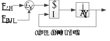
III. CONTROL SYSTEM
A bump-less override control system has been designed for the engine which is compatible with the typical engine control logics as shown in Fig. 9. Since thrust cannot be measured, the main control variable is fan speed which correlates with thrust. Operating the engine at its highest efficiency requires that all components operate at mechanical or thermal limits for at least one of the engine's critical operating conditions[11]-[12]. Limit controllers have been implemented to limit fuel flow to protect the engine against surge/stall, temperature, over-speed and over-pressure. In addition, setting a minimum fuel flow prevents blowout of the combustor.
Fig. 9. Engine Control architecture
The various control gains are determined by using linear engine models and linear control theory and are adjusted to provide the desired performance based on engine ground and altitude tests. Proportional and integral control (PI) is sufficient for providing good fan speed tracking.
The fuel system has been modelled as a lag time constant which represents the delay due to fuel transfer in the pipe from the valve to the combustion chamber in addition to that of the valve and actuator.
IV. RESULTS
This section presents the performance plots of key dynamic and steady-state tests. Maps from TMATS [13] of Pratt & Whitney JT9D engine have been implemented for simulation purposes. Two sets of results are presented at two altitude levels and different Mach numbers. Time responses of relative
+- FAN Speed controller 1s
Limit controllers
HPC shaft speed
M
in Max
Blowout controller HPC discharge pressure
Engine HPT outlet temperature
HPC discharge pressure
FAN Speed Demand
Hf
H
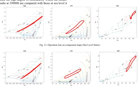
[image:3.596.319.541.399.491.2] [image:3.596.77.275.644.688.2]thrust are shown in Fig. 10 and Fig. 11. The results depicted in Fig. 12 and Fig. 13 are the dynamic performance of the engine under rapid acceleration and deceleration.
[image:4.596.81.239.95.310.2]Fig. 10. Relative thrust time response (Sea Level Static)
Fig. 11. Relative thrust time response (35000 ft, Mach Number 0.8)
The operation lines shown in in Fig. 12 and Fig. 13 demonstrate the high degree of nonlinearity within the model. If the results at 35000ft are compared with those at sea level it
can clearly be seen that the operation of the engine depends on altitude level.
Surge in LPCs at high altitudes during deceleration is highly probable. For this reason a surge limit controller saturates the fuel command derivative before the free integrator within the control system. This can be seen in Fig. 11 which shows the thrust time response is nonlinear while in Fig. 10 it can be approximated as a first order system for engine operation at sea level.
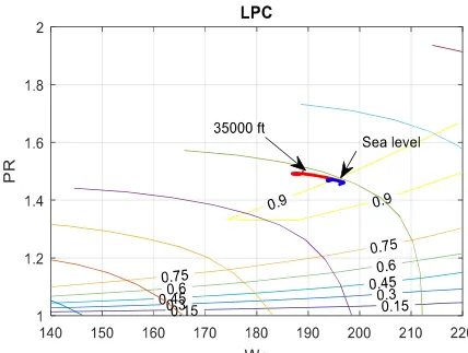
Fig. 14, Fig. 15 and Fig. 16 illustrate the impact of 1 MW power off-take from the LP and HP shafts on the HPC and LPC performance at sea-level and at 35000ft. Fig. 14 shows that at higher altitudes power off-take from LP-shaft increases HPC speed, which means there is a limit on power off-take at higher altitudes. If the speed exceeds the maximum permissible speed stresses and vibrations in the compressor will cross the prescribed limit, and this can damage the compressor.
[image:4.596.83.238.221.324.2]Power off-take from HP shaft solves this problem by decreasing the HPC speed and mass flow (Fig. 15). However, this could indirectly cause surge since the LPC performance point naturally moves closer to surge line (Fig. 16). Overall, the analyses performed show that for future studies on more electric aircraft there is a limit on power off-take for each shaft at different altitudes.
Fig. 12. Operation line on component maps (Sea Level Static)
[image:4.596.69.526.368.651.2]Fig. 14. Effect of 1 MW power off-take from LP shaft on HPC map
Fig. 15. Effect of 1 MW power off-take from HP shaft on HPC map
Fig. 16. Effect of 1 MW power off-take from HP shaft on LPC map
V. CONCLUSION
This paper has presented a nonlinear model a turbofan engine which has been developed for use with a future Integrated Power Center. The model allows power exchange between the engine shafts via starter-generator electrical
machines. The model has been evaluated at sea-level and 35000ft with two aircraft speeds. The results show that the engine response to acceleration and deceleration highly depends on the altitude. Analysis of compressor maps has shown that for future studies on more electric aircraft, there is a limit on the power off-take for different shafts at different altitudes and at different shaft speeds.
For future work, this model will be used in conjunction with an Integrated Power Centre to investigate optimized operation depending on Engine Operating Mode and control of the Electric Power System.
VI. REFERENCES
[1] M. J. Provost, “The More Electric Aero-engine: a general overview from an engine manufacturer,” in Power Electronics, Machines and Drives (PEMD2002),International Conference on(Conf. Publ. No. 487), 2002, pp. 246-251.
[2] H. Balaghi Enalou and E. Abbasi Soreshjani, “A Detailed Governor-Turbine Model for Heavy-Duty Gas Governor-Turbines With a Careful Scrutiny of Governor Features, ” in IEEE Transactions on Power Systems, vol. 30, no. 3, pp. 1435-1441, May 2015.
[3] Martin, S. (2009), “Development and Validation of a Civil Aircraft Engine Simulation Model for Advanced Controller Design” , PhD thesis, University of Leicester.
[4] J. F. Sellers and C. J Daniele, “DYNGEN-A program for calculating steady state and transient performance of turbojet and turbofan engines,” NASA Technical Report, no. NASA TN D-7901, 1975. [5] K. Parker and T. H. Guo, “Developement of turbofan engine
simulation in a graphical simulation environment,”NASA Technical Report, no. NASA TM 2003-212543, 2003.
[6] Jonathan A. DeCastro, Jonathan S. Litt, and Dean K. Frederick, “A modular aero-propulsion system simulation of a large commercial aircraft engine,” NASA Technical Report, no NASA TM 2008-215303, 2008.
[7] W. X. Zhou, J. Q. Huang and J. P. Duo, “Development of component level model for a turbofan engine,” in Journal of Aerospace Power, 21 (2), pp. 248–253, 2006.
[8] N. U. Rahman and J. F. Whidborne, “A numerical investigation into the effect of engine bleed on performance of a single-spool turbojet engine,” in Journal of Aerospace engineering, part G, 222 , pp. 939– 949, 2008.
[9] MATLAB, The Language of Technical Computing, Version R2015b, SIMULINK, Dynamic system Simulation for MATLAB, Version R2015b.
[10] https://en.wikipedia.org/wiki/Turbofan
[11] P.P Walsh and P. Fletcher. Gas Turbine Performance. Blackwell Science, 1sted, 1998.
[12] H Austin Spang III, Harold Brown, Control of jet engines, Control Engineering Practice, Volume 7, Issue 9, September 1999, pp. 1043-1059
[image:5.596.60.274.456.618.2]![Fig. 2. Schematic diagram of a two-spool high-bypass turbofan [10]](https://thumb-us.123doks.com/thumbv2/123dok_us/8600288.372431/1.596.339.532.233.390/fig-schematic-diagram-spool-high-bypass-turbofan.webp)