Step Free Energy The equilibrium shape of a hexagonal lattice

(1)

Bachelor Thesis

Step Free Energy

The equilibrium shape of a hexagonal lattice

Author:

Jasper Jonker

March 28, 2017

Physics of Interfaces and Nanomaterials

(2)

Chairperson: Prof. dr. ir. H.J.W. Zandvliet Daily supervisor: Prof. dr. ir. H.J.W. Zandvliet External member: Prof. dr. ir. J.E. ten Elshof

Jonker, Jasper: Step Free Energy

(3)

Abstract

This thesis derives an expression of the step free energy for the hexagonal lattice in the armchair and zigzag direction. This solid-on-solid model with nearest neighbor interaction recaptures the exact result of Wannier in case the armchair edge is consid-ered. The derivation of an exact expression for the edge free energy in the zigzag edge was attempted, but we did not manage to find it. The angular dependence of the step free energy is derived and with the use of the Wulff construction the equilibrium shape at different temperatures is determined.

Acknowledgements

(4)

List of Figures

1 Step energy in the [10] and [11] direction. For a graphical representation how the partition function is formed, see appendix D.1 . . . 3 2 F(T, φ) between φ= 0◦,5◦,10◦,15◦,20◦,25◦,30◦,35◦,40◦ and 45◦. Tc is the

order - disorder phase transition temperature (thermal roughening tempera-ture). . . 5 3 Step edge energy of the armchair and zigzag direction. It is seen that there

are many routes possible to form an armchair step edge, but only two routes are possible to form a zigzag step edge. For a graphical representation how the partition function is formed, see appendix D.2 . . . 7 4 The free energy of the armchair and the zigzag direction over temperature.

The armchair is anexact solution, however the zigzag is not since it does not end at Tc. . . 8 5 nis defined for the armchair and zigzag direction to be left. This is used to

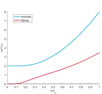
calculatehn2i. . . 10 6 Mean square kink length of a hexagonal lattice versus temperature for the

armchair and zigzag direction pera2. . . 11 7 The free energy is divided into two different directions,√3(n−m) segments

in the zigzag direction and 2m segments in the armchair direction. . . 12 8 F(T, φ) for a hexagonal lattice whereφranges from 0◦ to 30◦. Tcis the

ther-mal roughening temperature. F(T,0◦) is the zigzag direction and F(T,30◦) is the exact armchair direction as seen in fig. 4b. . . 13 9 Step edge boundary at 0◦, 30◦ and 60◦. This pattern keeps repeating itself. 14 10 Wulff plot at T = 0.01 Tc, T = 0.1 Tc and T = 0.4 Tc. The shape of the

crystal is represented by the interior and has transformed from a hexagon into a circle. The free energyF(T, φ) is on the radial axes and is represented by the dark blue line. . . 16 11 The routes represented by a black bar are counted twice in a√3/2 unit cell. 18 12 All different kink configurations in the [10] direction of the square lattice. . 24 13 All different kink configurations in the [11] direction of the square lattice. . 25 14 All different kink configurations in the armchair direction of the hexagonal

(6)

List of Symbols

Symbol Description Unit

F Helmholtz free energy J

G Gibbs free energy J

H Enthalpy J

P Pressure N·m−2

S Entropy J·K−1

Tc Thermal roughening temperature K

T Temperature K

U Internal energy J

V Volume m3

Z Partition function

β∗ Step edge stiffness

β 1/kbT J−1

Interaction energy J

γ Free energy J

hn2i Mean square kink length m2

a Lattice constant m

(7)

1 Introduction

Statistical mechanics is often used to describe the state of a system by the use of probability theory. One statistical model invented by Lenz [1] was a theoretical description of ferromag-netism. Ising, a student of Lenz, was able to solve the one dimensional Ising model in his thesis in 1924 [2]. He showed that in the one dimensional model no phase transitions occur. Because of this, he asserted that there are no phase transitions in two and three dimensions.

This discouraged Ising from pursuing to higher dimensions. However, Onsager solved the two dimensional Ising model much later using the transfer-matrix method in 1944 [3]. On-sager showed that Ising’s assertion was wrong for all higher dimensions. A two dimensional lattice already identifies a phase transition at a certain temperature.

This was a very important discovery which completely changed the developments of sta-tistical mechanics. Before Onsager’s result, it was not clear if the models in stasta-tistical mechanics were able to handle phase transitions.

In this treatise on the step free energy, a different approach is used than Onsager to find the same exact answer. The partition function is used to take into account all possible kinks in the lattice. The partition function gives the free energy versus temperature.

The state of a surface at or near (local) equilibrium is quite different than a non-equilibrium surface. This thesis is only on equilibrium surfaces.

This thesis is structured as follows: chapter two introduces edge free energies. A square lattice is used to review the model and an equation of the free energy versus temperature is presented. The square lattice is solved exactly and is used as an introduction to the hexagonal lattice.

(8)

2 Anisotropic Square Lattice

The equilibrium shape of a two dimensional island is directly related to the magnitude of the step free energy [4]. The step free energy is used as a fundamental quantity that describes the thermal fluctuations of the steps and how they are arranged on the surface. The step free energy is defined as the free energy to create a crystal step edge [5]. As it will be shown, the step free energy will decrease with increasing temperature due to the meandering entropy. The free energy is related by

F =U −T S, (1)

withF the free energy in joules,U the internal energy in joules,T the temperature in kelvin and S the entropy in joules per kelvin. At a certain temperature Tc, F = 0, where steps will be generated spontaneously1. IfTc is below the melting temperature, the formation of domain boundary can be observed experimentally [6].

The kink creation energy is /2 or half the nearest-neigbor interaction energy. In the anisotropic square lattice the interaction energy is different in thex and y direction. For the isotropic lattice, x =y. In the square lattice, two different phase boundaries can be formed, the [10] and the [11] direction (fig. 1). The goal is to find the phase boundary at any angle.

2.1 [10] direction

To find the energy to form a phase boundary spontaneously, the partition function2 of the system has to be found. In the partition function all the possible kink formations are included. When looking at figure 1a, the boundary formation energy of one elementary unit ain the [10] direction isx/2 and in the [01] direction y/2. The path with the lowest energy is x/2, however there are many more higher energy paths. These paths are called kinks. The first kink has an energy of x/2 +y/2 and the second kink has an energy of

x/2 + 2y/2 and so on. Using Boltzmann statistics, the partition function becomes

Z[10]= exp

₋

x 2kbT

(

1 + 2 ∞ X n=1 exp ₋ ny 2kbT

)

= exp

₋

x 2kbT





1 + exp−y

2kbT

1−exp−y

2kbT



. (2)

Since kinks can be formed in the +y direction and the−y direction a factor 2 is included in eq. (2). One elementary unit of ais considered.

1_{For more information, see appendix A} 2

(9)

[image:9.595.96.502.98.317.2]

(a) Step energy in the [10] direction. (b) Step energy in the [11] direction.

Figure 1: Step energy in the [10] and [11] direction. For a graphical representation how the partition function is formed, see appendix D.1

2.2 [11] direction

A step in the [11] direction costs x/2 or y/2 as seen in figure 1b. The energy for the first kink is x/2 +y/2 plus x/2 ory/2. The second kink has a total energy of 2 (x/2 +y/2) plus x/2 ory/2. The total partitions sum can be written as

Z_[11]= ∞

X

n=0 exp

₋

n(x+y) 2kbT

exp

₋

x 2kbT

+ exp

₋

y 2kbT

=

exp−x

2kbT

+ exp−y

2kbT

1−exp−(x+y)

2kbT

.

(3)

(10)

2.3 Critical temperature

The critical temperature, also called thermal roughening temperature, Tcis found when the free energy is zero. The relation between the partition sum and the free energy is

F =−kb T ln(Z). (4)

When the partition function Z equals one, the free energy F is zero. In both directions (eqs. (2) and (3)) Onsager’s [3] order-disorder phase transition temperature of the 2D square Ising model is recaptured.

sinh

x 2kbTc

sinh

y 2kbTc

= 1 (5)

2.4 Free energy for an arbitrary angle

To find the free energy at any angle, the boundary is divided into N-M [10] elements and M [11] elements. This means there are N total steps of which N-M in the [10] direction since the angle between the [10] and the [11] direction is 45◦. The total partition function is then given by Ztot = (Z[10])N−M(Z[11])M and the angle by tanφ= (M/N).

F(T, φ) then becomes [7]

F(T, φ) =−1

LkbT

n

ln Z[10]

N−M

+ ln Z[11]

Mo

(6)

WhereN−M =N(1−tanφ) andM =Ntanφ. The partition functionZ_[11]is taken over two elementary units of 1₂√2a. The energy at T = 0K in theZ[11] direction is /

√

2 per a

and the energy in the Z_[10] direction is /2 pera. The total step edge lengthL is

L= (N −M)a+M√2a=N an(1−tanφ) +√2 tanφo (7)

Combining eqs. (2), (3), (6) and (7) gives

(8)

F(T, φ) =−kbT

 



(1−tanφ) (1−tanφ+√2)ln





exp

−x

2kbT

n

1 + exp

₋

y

2kbT

o

1−exp

₋

y

2kbT





+ 2 tanφ

(1−tanφ+√2)ln





exp

−x

2kbT

+ exp

₋

y

2kbT

1−exp

₋₍

x+y)

2kbT

    

As can be seen in fig. 2, the energy at T = 0K corresponds with /√2 ≈0.71 at 45◦ and

(11)

[image:11.595.160.423.274.490.2]

(12)

3 Hexagonal Lattice

In the previous chapter, the square lattice was discussed as an introduction to the hexagonal lattice. There are two directions in the hexagonal lattice one can specify, the armchair (fig. 3a) and the zigzag (fig. 3b). For both directions a partition function is found that is used to determine the step free energy. The mean square length is determined to find the average squared distance of a kinked boundary. Finally, the free energy at an arbitrary angle is used to form the Wulff plot and determine the equilibrium shape of the crystal.

3.1 Isotropic armchair

The partition function in the [10] direction is (see fig. 3a) [8]

Zarm= 2 ∞ X n=1 exp − n

kbT

=

2 exp_k−

bT

1−exp_k−

bT

(9)

The step edge free energy can be written as

Farm=−kbTln





2 exp_k−

bT

1−exp_k−

bT



 (10)

This result is plotted in figs. 4a and 4b.

3.2 Anisotropic armchair

The partition function in the armchair direction for a anisotropic hexagonal lattice is given by

Zanarm = exp

₋

1 2kbT

exp

₋

2 2kbT

+ exp

₋

3 2kbT

∞ X

n=0 exp

₋

n(2+3) 2kbT

=

exp−(₂_k1+2)

bT

+ exp−(1+3) 2kbT

1−exp−(₂_k2+3)

bT

(11)

The routes to include are the same as for the isotropic case, but the interaction energy is different for all three directions. WhenZanarm= 1, the result is

exp

−(1+2) 2kbTc

+ exp

−(1+3) 2kbTc

+ exp

−(2+3) 2kbTc

= 1 (12)

When 1=2 =3 =the result of Wannier [9] in 1945 is obtained

kbTc

(13)

3 Hexagonal Lattice

(a) The armchair direction in a hexagonal lat-tice. The two shortest routes possible have energy1/2 +2/2 and1/2 +3/2. However,

there is an infinite amount of routes.

[image:13.595.98.497.103.300.2]

(b) The zigzag direction in a hexagonal lat-tice. Within the two lines, there are two routes possible with energy/2 and the other route costs.

Figure 3: Step edge energy of the armchair and zigzag direction. It is seen that there are many routes possible to form an armchair step edge, but only two routes are possible to form a zigzag step edge. For a graphical representation how the partition function is formed, see appendix D.2

3.3 Isotropic zigzag

Until now, I have not found an exact solution for the zigzag direction in a hexagonal lattice. The problem that arises in a √3a/2 unit is that there are only two different directions possible (fig. 3b). More routes can be included, but parts of those routes are counted more than once.

In one elementary unit of √3a/2, shown in fig. 3b, the partition function from A to the next line gives

Zz = exp

₋

2kbT

+ exp

₋

kbT

. (14)

No routes are counted more than once in this partition function. The free energy of Zz is plotted in fig. 4a. It can be seen that not all routes are included since it overshoots Tc at

(14)

3 Hexagonal Lattice

Zzig=

exp

₋

2kbT

+ exp

₋

kbT

∞ X n=0 exp ₋ 4n

2kbT

=

exp₂−_k

bT

+ exp_k−

bT

1−exp−2_k

bT

. (15)

(a) The free energy for only 2 paths, given in fig. 3b. As seen the zigzag direction is far of from pointTc.

[image:14.595.86.513.128.355.2]

(b) More routes (eq. (15)) are included which results in a graph of the zigzag direction that is slightly beforeTc.

Figure 4: The free energy of the armchair and the zigzag direction over temperature. The armchair is an exact solution, however the zigzag is not since it does not end atTc. The values at T = 0 K can be found for the armchair and the zigzag direction. For the armchair direction, two bonds are broken every 3a. Therefore at T = 0 K the armchair direction should start at /3. For the zigzag direction there is one bond broken every√3a. Therefore the graph in fig. 4a should start at

2√3 ≈0.288.

3.4 Mean square kink length armchair

The meandering of a step can be represented by the mean square length. hn2i is sometimes referred as the diffusivity of the domain wall. The mean square kink length is the expec-tation value of the square kink length. hni can be calculated as well, but this will average out to zero since positive and negative kinks are substracted from each other.

(15)

3 Hexagonal Lattice

P0= exp

₋

kbT

P1 = exp

− kbT

P−1= exp

−2 kbT

P2 = exp

−2 kbT

P−2= exp

−3 kbT

.

(16)

The mean square kink length can therefore be expressed as

hn2i= 1

Zarm ∞

X

n=−∞

n2Pn= 1

Zarm

( _∞ X

n=1

n2exp

−(n+ 1)

kbT

) + 1 Zarm ( _∞ X n=1

n2exp

− n

kbT

)

,

(17)

where Zarm is defined in eq. (9). The distance between every step n is

√

3a, thus 3a2 for

n2. This is per 3/2a, therefore hn2i is per 1/2a . This results in

hn2i_arm= 2





1 + exp_k−

bT

1−exp_k−

bT   2 (18)

This result of hn2i in the armchair direction is shown in fig. 6.

3.5 Mean square kink length zigzag

The same procedure is applied for the zigzag direction. The routes to include are (see fig. 5b)

P0 = exp

−

2kbT

P2 = exp

−2

2kbT

P−3 = exp

−5

2kbT

P5 = exp

₋

6

2kbT

P−6 = exp

₋

9

2kbT

P8 = exp

₋

10

2kbT

P−9 = exp

₋

13

2kbT

(16)

3 Hexagonal Lattice

(a) The armchair direction where n goes from−∞to +∞.

[image:16.595.100.498.103.298.2]

(b) The zigzag direction in a hexagonal lattice where n goes from−∞to +∞.

Figure 5: n is defined for the armchair and zigzag direction to be left. This is used to calculate hn2i.

This can be expressed as

hn2i= 1

Zzig

( _∞ X

n=0

(2 + 3n)2exp

₋

(4n+ 2)

2kbT

) + 1 Zzig ( _∞ X n=0

(3n)2exp

₋

(4n+ 1)

2kbT

)

=

exp_k−

bT

h

4 + 5 exp−2_k

bT

+ exp−4_k

bT

+ 9 exp₂−3_k

bT

+ 9 exp₂−7_k

bT

i

h

exp₂−_k

bT

+ exp_k−

bT

i h

1−exp−2_k

bT

i2

(20)

Where Zzig is defined in eq. (15). The distance between each nis exactly a. The distance between each half unit cell is √3/2. The mean square length is therefore multiplied by 2/√3, giving hn2_i_per _a2

hn2izig=

2 exp_k−

bT

h

4 + 5 exp−2_k

bT

+ exp−4_k

bT

+ 9 exp₂−3_k

bT

+ 9 exp₂−7_k

bT i √ 3 h exp − 2kbT

+ exp

− kbT

i h

1−exp

−2 kbT

i2 (21)

(17)

[image:17.595.130.464.213.520.2]

3 Hexagonal Lattice

(18)

3 Hexagonal Lattice

3.6 Free energy for an arbitrary angle

[image:18.595.104.494.190.344.2]

The free energy at any angle in a hexagonal lattice can be expressed using the two solutions of the armchair and zigzag direction found in sections 3.1 and 3.3. The armchair direction makes an angle of 30◦ with the zigzag direction, see fig. 7.

Figure 7: The free energy is divided into two different directions, √3(n−m) segments in the zigzag direction and 2m segments in the armchair direction.

The partition function is written as a product of two different orientations. There are

√

3(n−m) segments in the zigzag direction and 2m segments in the armchair direction.

Ztot= (Zzig) √

3(n−m)

(Zarm)2m=

n

(Zzig) √

3−3 tanφ

(Zarm)2 √

3 tanφon

(22)

Where Ztot is the total partition function, tanφ= _nm√₃ (φ∈[0◦,30◦]). The total step edge length is

L=

√

3 (n−m)1 2

√

3a+ 6m a=n a

3 2

1−√3 tanφ

+ 6

√

3 tanφ

(23)

The total step edge energy is

Ftot=−kbTln (Ztot) =−

√

3(n−m)kbTln (Zzig)−2mkbTln (Zarm) (24) The step edge energy per unit length ais given by

F = −kbT

√

3−3 tanφ

ln (Zzig) + 2

√

3 tanφ ln (Zarm)

3 2 1−

√

3 tanφ+ 6√3 tanφ (25)

(19)

3 Hexagonal Lattice

F(T, φ) =−kbT

√

3−3 tanφ

/2

₃

2 1−

√

3 tanφ

+ 6√3 tanφln 



exp₂−_k

bT

+ exp_k−

bT

1−exp−2_k

bT





−kbT

2√3 tanφ

₃

2 1−

√

3 tanφ+ 6√3 tanφln





2 exp

− kbT

1−exp

− kbT





(26)

[image:19.595.132.496.266.469.2]

Figure 8 is a plot of F(T, φ) versus temperature for different angles.

(20)

3 Hexagonal Lattice

3.7 Wulff plot

The Wulff construction [10] is used to determine the equilibrium shape of the crystal. The equilibrium shape must minimize the excess surface free energy3.

The Wulff construction is performed as follows: for each orientation φ, draw a line ˆnfrom the origin to the surface ofF(φ, T). When the radial line intersectsF(φ, T), a perpendicular line to ˆn is drawn. The interior of the envelope that results from all those perpendicular lines is the minimizing shape for an isolated volume.

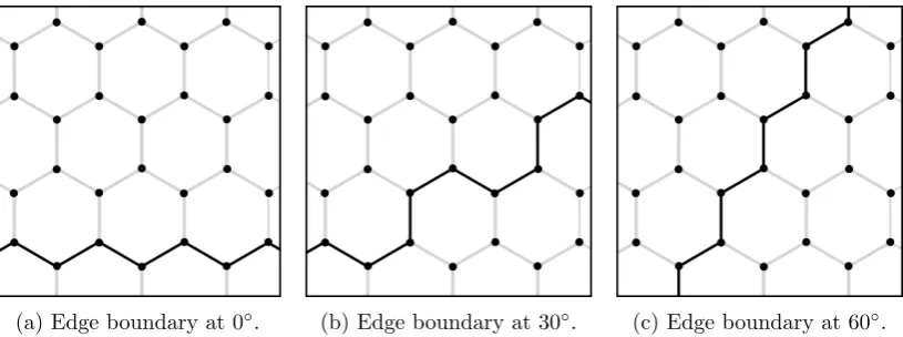
The free energy in section 3.6 is determined for φ∈[0◦,30◦]. The free energy, F(T, φ) from 0◦ to 360◦ can be found by using fig. 9. F(T, φ) is fully governed by the zigzag direction at 0◦ and transforms into the armchair direction at 30◦. At 60◦ the free energy is fully governed by the zigzag direction again. This repeats itself 5 more times. The free energy is therefore

F(T, φ) φ∈[0◦,30◦]

F(T,30◦−φ) φ∈[30◦,60◦]

and continues in this manner till 360◦.

[image:20.595.95.503.419.571.2]

(a) Edge boundary at 0◦. (b) Edge boundary at 30◦. (c) Edge boundary at 60◦.

Figure 9: Step edge boundary at 0◦, 30◦ and 60◦. This pattern keeps repeating itself.

(21)

3 Hexagonal Lattice

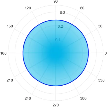
The Wulff plot is shown in fig. 10. AtT = 0.01Tcthe equilibrium shape is a hexagon, while it transforms into a circle around T = 0.4Tc. From fig. 8 it can be seen thatF(T,0◦) and

F(T,30◦) are coming together at T = 0.4 Tc. When the free energy in both directions is the same at a certain temperature, the equilibrium shape is a circle. Since the free energy should be zero at the same time for both directions (at Tc), the equilibrium shape of a crystal will always become a circle at Tc.

However, the free energy of the step edge in zigzag direction is an approximation and therefore will not end up exactly in Tc. The shape of the crystal at Tc, according to this approximation, will not be a perfect circle.

(a) The Wulff plot at T = 0.01 Tc. The equilibrium shape of the crystal is a

(22)

3 Hexagonal Lattice

(b) The Wulff plot at T = 0.1Tc. The edges of the equilibrium shape

of the crystal are becoming rounder.

(c) The Wulff plot at T = 0.4Tc. The equilibrium shape of the crystal

[image:22.595.195.403.381.588.2]

is an almost perfect circle.

(23)

3 Hexagonal Lattice

3.8 Step edge stiffness

The relation between the mean square length and the stiffness β∗(T) is given by

β∗(T) = a 2

hn2_i (27)

The step edge stiffness is determined for low temperatures (T ≈0). Each direction has its own stiffness. The mean square length pera2 of the armchair direction is given in eq. (18). At low temperatures this reduces to

β∗(T)arm= 1

2. (28)

For the zigzag direction the mean square length was calculated in eq. (21). In the limit of

T = 0 the mean square length becomes zero. Therefore the stiffness is

(24)

4 Discussion and Recommendations

Many attempts were taken to find the exact solution in the zigzag direction. The first attempt was to include only the two most self-evident routes. This was a very low approx-imation. It was only valid at very low temperatures. Therefore, a better route had to be found. However, the first problem that arises is the determination of what route can be included. In a √3/2 cell, as in fig. 3b, coming back to the starting point will increase the chance of double counting. In the partition function that is used for the zigzag direction some routes are counted twice. Figure 11 shows the double counting boundary edges in the

√

[image:24.595.124.473.252.321.2]

3/2 unit cell with the zigzag partition function found in eq. (15).

Figure 11: The routes represented by a black bar are counted twice in a √3/2 unit cell.

In the history of the partition function, i.e. the previous √3/2 unit cell, some boundary lines are included which are counted in the next partition function as well. The partition function includes more energy than required to form these boundaries.

However, the free energy is less than 2.5% off from the exact value ofTcin the armchair di-rection. Figure 4b shows that the zigzag direction is very close toTc. Since both directions should end in Tc whenF = 0, the approximation is very accurate.

The mean square kink length was found for the armchair and zigzag kink direction. The armchair has two routes of the same energy from the starting point. The kink length is therefore larger than 0 at T = 0. However, the zigzag direction will not form any kink boundary at T = 0, since all other paths than the 0 path have higher energies.

(25)

4 Discussion and Recommendations

4.1 Recommendations for further research

Future research in step edge energies should search for an exact solution in the hexagonal lattice. However, using the method described in this thesis might not give the exact answer in the zigzag direction. Other methods have to be incorporated as well.

The Ising model is solved for one and two dimensions, but not for three dimensions yet. However, three dimensions brings many more challenges. For a one dimensional line, there are 2 nearest neighbors, for a square lattice there are 4 nearest neighbors and in a cube lattice there are 6 nearest neighbors. It becomes very hard to locate all directions of the meandering entropy in three dimensions.

(26)

5 Conclusion

This thesis started with an introduction to the Ising model using only nearest neighbor interaction in a square lattice. The free energy is derived with full angular dependence. The method used is different than Onsager did in his article [3], however it does show the same exact result.

In chapter three the hexagonal lattice in analyzed. The partition function for both directions was found. The armchair edge is an exact solution and the zigzag edge is an approximation. The approximation is less than 2.5% off from Tc. The mean square length or diffusivity of the domain wall is calculated. As temperature increases, the mean square length increases and has a finite value at Tc.

The free energy is derived for any angle in the hexagonal lattice. This was done to find the shape of the crystal in equilibrium using the Wulff construction. Around T ≈ 0 K

the shape of the material will form a hexagon in equilibrium. When the temperature is increased towards T ≈0.4 Tc the crystal is almost a perfect circle. The free energy of the zigzag and armchair edge do not reach the same temperature at F = 0. This is due to the approximation used for the zigzag edge. However, the crystal should be a perfect circle at

(27)

A Phase transitions

A

Phase transitions

When changing any of the macroscopic variables of a system, sometimes its properties abruptly change. This might be a change from solid to liquid, but also solid to solid phase transitions occur. When do these phase transitions occur?

Looking closely to water, many would say it has only three phases: solid, liquid and gas. However, water has at least 15 experimentally confirmed solid phases [13]. Each of them have different arrangements of the atoms in the crystal.

To determine the phase with the largest probability, one can look at the phase diagram of the material. However, F = U −T S where at low temperatures the free energy is de-termined by the internal energy. The solid phase will be most stable since each molecule is hold tightly in its place. It is a very low entropy state because the molecule is at fixed positions.

In the liquid phase, a water molecule is more freely and they are constantly forming and breaking bonds and moving around. The molecules are not at fixed positions. Therefore, the liquid phase has a higher energy state and a higher entropy state compared to the solid phase.

The molecules in the gas phase are much more mobile than in the liquid phase. There are almost no bonds between the molecules. Therefore, the energy and the entropy are much higher in the gas phase.

At higher temperatures, the entropy term starts to increase. The entropy term becomes much more important. Before a phase transitions occurs, the free energy between the two phases becomes smaller. When those energies are exactly equal, the phases have equal probabilities. However, latent heat must be put in the system before it is transformed into that phase.

When a system has the system variables P and V, one can use the Gibbs free energy to calculate a phase transition.

U1+P V1−T S1 =U2+P V2−T S2 (30)

(28)

B Partition function

B

Partition function

The partition function is the most important tool in statistical mechanics. It provides information about the state variables entropy, temperature, free energy and total energy and more. The partition function in a discrete canonical ensemble is described as

Z =X

i exp

− Ei

kbT

. (31)

It is a sum over all exponential microstate energies. But what statistical meaning does the partition sum has? The probability that the system is in a certain microstate iis given by

Pi = 1

Z exp

− Ei

kbT

. (32)

The negative sign in the exponential shows that a state with a lower energy has a higher probability. There is a link from the microscopic system to the macroscopic system. This is given by

U =hEi=X i

EiPi = 1

Z

X

i

Eie−βEi =− 1

Z ∂ ∂β

X

i

e−βEi ₌₋∂lnZ

∂β (33)

With β = 1/(kbT). U is the internal energy of the system. The free energy can be found from the partition function using F =−kbTln(Z). Now it is fairly easy to show what the entropy of the system is. The Helmholtz free energy is equal to

F =U−T S (34)

(29)

C Equilibrium crystal shape

C

Equilibrium crystal shape

The thermodynamic free energy is the energy in a system that can be converted to do work. The Helmholtz free energy F = U −T S is the energy that can be converted into work at a constant temperature and volume (isothermal and isochoric). The Gibbs free energy

G =H −T S is the energy that can be converted into work at constant temperature and pressure (isothermal and isobaric). H is the enthalpy, given by H =U +P V, with P the pressure andV the volume [14]. Whether to use Helmholtz free energy or Gibbs free energy depends on the system. In this thesis, constant temperature and volume criteria of the system and therefore the Helmholtz free energy is used. Besides, the Helmholtz free energy is directly related to the partition function and is therefore easier to work with.

The shape of a crystal in a well defined equilibrium requires it to avoid any contact with the wall, surface or atmosphere [15]. Gibbs is generally credited for being the first to show that a crystal will rearrange itself to the minimum integrand of the surface free energy over the whole surface [16].

Z

γ dA is minimum. (35)

With γ the free energy. Wulff [10] was the first who showed how the shape can be calcu-lated from the surface free energy, nowadays known by the Wulff construction. However, his proof was incorrect. Dinghas [17] gave a proof which was extended to any arbitrary shape by Herring [18, 19].

The equilibrium used in this context is for a constant volume and temperature, and there-fore the goal is to minimize the Helmholtz free energy. As presented in section 3.7, the shape is the inner envelope of the surface of the planes perpendicular to the radii of the surface free energy polar plot.

(30)

D Graphical representation of the partition function

D

Graphical representation of the partition function

D.1 Square lattice

The partition function found in the square lattice is represented graphically in fig. 12. By showing all possible kink configurations the partition function can be found by including all of those energies. Since each term with higher energy is less probable according to the Boltzman distribution, the sum converges.

(a) First boundary with en-ergyx/2.

(b) First kink with energy x/2 +y/2.

(c) Second kink with energy x/2 +y.

(d) Third kink with energy x/2 + 3y/2

[image:30.595.92.503.212.555.2]

(e) All kink configurations de-scribed in the partition function.

(31)

The same can be done in the [11] direction.

(a) First boundary with energy (x/2 or

y/2).

(b) First kink with energy (x/2 +y/2)

+ (x/2 ory/2).

(c) Second kink with energy 2 (x/2 +

y/2) + (x/2 ory/2).

[image:31.595.119.478.129.528.2]

(d) All different kink configuration de-scribed in the partition funcion.

(32)

D.2 Hexagonal lattice

(a) First kink with energy E1=.

(b) Second kink with energy E2=.

(c) Third kink with energy E3= 2.

(d) Fourth kink with energy E4= 2.

[image:32.595.94.504.132.470.2]

(33)

(a) First kink with energy E1=/2.

(b) Second kink with energy E2= 2/2.

(c) Third kink with energy E3= 5/2.

(d) Fourth kink with energy E4= 6/2.

[image:33.595.92.502.102.654.2]

(34)

References

[1] W. Lenz. Z. Phys., 21:613, 1920.

[2] Ernst Ising. Contribution to the Theory of Ferromagnetism. Z. Phys., 31:253–258, 1925.

[3] Lars Onsager. Crystal statistics. i. a two-dimensional model with an order-disorder transition. Phys. Rev., 65:117–149, Feb 1944.

[4] N. C. Bartelt, R. M. Tromp, and Ellen D. Williams. Step capillary waves and equilib-rium island shapes on si(001). Phys. Rev. Lett., 73:1656–1659, Sep 1994.

[5] H. J. W. Zandvliet. Determination of ge(001) step free energies.Phys. Rev. B, 61:9972– 9974, Apr 2000.

[6] Kai Sotthewes and Harold J W Zandvliet. Universal behaviour of domain wall mean-dering. Journal of Physics: Condensed Matter, 25(20):205301, 2013.

[7] H.J.W. Zandvliet. Step free energy of an arbitrarily oriented step on a rectangular lattice with nearest-neighbor interactions. Surface Science, 639:L1–L4, 2015.

[8] H.J.W. Zandvliet. The 2d ising square lattice with nearest- and next-nearest-neighbor interactions. Europhysics Letters, 73(5):747–751, 2006.

[9] G. H. Wannier. The statistical problem in cooperative phenomena. Rev. Mod. Phys., 17:50–60, Jan 1945.

[10] G. Wulff. Zur Frage der Geschwindigkeit des Wachsthums und der Aufl¨osung der Krystallfl¨achen, volume 34. 1901.

[11] R. L. Dobrushin, R. Koteck´y, and S. B. Shlosman. Wulff Construction:A Global Shape From Local Interaction.

[12] Ronny Van Moere, Harold J. W. Zandvliet, and Bene Poelsema. Two-dimensional equilibrium island shape and step free energies of cu(001). Phys. Rev. B, 67:193407, May 2003.

[13] Burkhard Militzer and Hugh F. Wilson. New phases of water ice predicted at megabar pressures. Phys. Rev. Lett., 105:195701, Nov 2010.

[14] Daniel V. Schroeder. Introduction to Thermal Physics. TBS, 1999.

[15] T. L. Einstein. Equilibrium Shape of Crystals. ArXiv e-prints, January 2015.

(35)

References

[17] Alexander Dinghas. Über einen geometrischen satz von wulff für die gleichgewichtsform von kristallen. Zeitschrift für Kristallographie - Crystalline Materials, 105:304–314, 1943.

[18] Conyers Herring. Some theorems on the free energies of crystal surfaces. Phys. Rev., 82:87–93, Apr 1951.

[19] C. Herring. The Use of Classical Macroscopic Concepts in Surface Energy Problems. In R. Gomer and C. S. Smith, editors,Structure and Properties of Solid Surfaces, page 5, 1953.