Joint reconstruction and motion estimation via nonconvex optimization for dynamic MRI

(1)

Joint reconstruction and

motion estimation

via nonconvex optimization

for dynamic MRI

MASTER THESIS W.A.P. BASTIAANSEN

Faculty of Electrical Engineering, Mathematics and Computer Science (EEMCS) Master program Applied Mathematics

Specialization: Systems Theory, Applied Analysis and Computational Science (SACS) Chair: Applied Analysis

Graduation committee: Prof. dr. S.A. van Gils (UT) Dr. C. Brune (UT)

Dr. ir. C.A.T. van den Berg (UMC Utrecht) Prof dr. ir. B.J. Geurts (UT)

Daily supervisor Dr. C. Brune

(2)

(3)

Abstract

Dynamic magnetic resonance imaging (MRI) is a medical imaging technique. MRI reconstruction methods build upon inverse problems, variational methods and optimization in applied mathematcis. To reduce scan-ning time in dynamic MRI, subsampling of the measurements is needed in practice. This typically leads to arte-facts due to missing information. To tackle those artearte-facts, time-dependent reconstruction methods, which employ not only the spatial properties of the image sequence, but also the dynamical information, are very promising.

In this thesis a joint reconstruction and motion estimation framework is developed and applied to dynamic MRI reconstruction. The optimization of this joint variational model is challenging since it is nonconvex. Cur-rent approaches alternate between the convex subproblems for reconstruction and motion estimation. This approach seems to be working but there is no knowledge about the convergence. To address this problem the full nonconvex model is optimized via an alternating forward-backward splitting algorithm which is related to the PALM algorithm for nonconvex optimization.

(4)

Acknowledgments

With this master thesis I conclude my time as a student applied mathematics. Six and a half years ago I exchanged the sunny south of the Netherlands (Brabant!) for the far east. I look back at my time as a student with a big smile on my face. I gained a lot of experiences I never thought I would. Running the final stage of the Batavierenrace, being a board member, being part of a ’dispuut’ and so on. For every EC I had to work hard, sometimes because the course was difficult and sometimes because I was giving myself a hard time. I am proud of what I achieved over the last years and this thesis feels like the cherry on the pie. I would not have achieved this without the help of many people.

First of all I would like to thank my supervisor, Christoph Brune, who introduced me to the field of imaging and encouraged me to work on this project. While I was working on my thesis, we had a lot of very good, sometimes really long, discussions. Afterwards I always was full of new ideas and inspiration (and to be honest a bit exhausted as well). Without Christophs enormous knowledge and enthusiasm this thesis would not have been what it is. I asked for a challenge, and that is what I got, but it is save to say he helped me to get the most out of it.

I also want to thank Stephan van Gils for welcoming me into the Applied Analysis group and always supporting my changing plans regarding my master program. Furthermore, I want to thank Yoeri for proofreading my thesis and giving very valuable feedback. I also want to thank Sophie, for being my study-buddy during our master courses, where we became, while discussing mathematics, really good friends.

In this acknowledgements I also want to mention my study advisor Lilian Spijker and (former) bachelor coordinator Brigit Geveling, I struggled a lot in the beginning of my study and without their guidance and support I probably would not have made it past my first year.

(5)

Chapter 1 Introduction

Since the discovery of Magnetic Resonance Imaging (MRI) in 1971 it is a well known form of medical imaging. MRI is based on the phenomenon called Nuclear Magnetic Resonance (NMR). In the presence of a strong mag-netic field protons will align with this field. When this magmag-netic field is turned off, the protons start spinning back to their original position and while spinning they send out a signal. An MR image reflects the intensity of this signal. As the proton density varies for different substances, we can see the structure of the body and abnormalities in an MR image. However this spinning will only happen at a specific strength of the magnetic field, so by creating gradients in the magnetic field we can measure specific positions. The advantage of MR imaging is that no radiation is involved so it will not harm the human body.

The signal received during data acquisition is the Fourier transform of the image, thus the signal has the fol-lowing form:

F(γGxt,γGyt)=

Z _∞

−∞

Z _∞

−∞

f(x,y)e−i2π[x(γGxt)+y(γGyT)]_d_x_d_y_,

wereF(_γGxt,γGyt) is the electromagnetic signal,f(x,y) the desired image andGxandGyare the gradients of the magnetic field. A clear derivation and more details can be found at [55]. Callkx=γGxtandky=γGy, data acquisition in MRI is often called sampling ink-space. If the number of measurements ink-space equals the resolution of the desired image, the inverse Fourier transform of the measurement will give the image. The limitation of MRI is that the measurement time is directly proportional to the number of measurements ink-space. Thus, to shorten the measurement time, subsampling is needed. However, subsampling leads to artefacts due to missing information, see Figure 1.1. As the measurement time for each point ink-space is limited by physical properties of the MRI scanner, research is mainly focused on reconstruction methods to overcome artefacts due to subsampling. Famous are parallel imaging and compressed sensing for static MRI reconstruction. Reconstruction techniques based on parallel imaging are SENSE [45] and GRAPPA [27], which make use of the fact that the spatial sensitivity for receiver coils varies for different positions of the coils in the MRI scanner. Compressed sensing [36] is based on the compressibility of images, by enforcing sparseness in an appropriate transform of the image.

(a) Ground truth image (b) Fully sampledk-space (c) Subsampledk-space (d) Direct inversion of

sub-sampled image

(7)

Dynamic MRI is used to capture objects in motion and offers a lot of opportunities. If we would be able to reconstruct fast enough, dynamic MRI could become real time. However dynamic MRI is even more time consuming than static MRI. A limitation in dynamic frame-by-frame reconstruction is the missing temporal information in the modeling. Examples where temporal information is modeled are the low-Rank plus sparse decomposition of [40], were the low-rank matrix captures the static background and the sparse matrix cap-tures the dynamic foreground. Another example is the ICTGV method of [48], which uses stronger temporal regularization for the background and stronger spatial regularization for the dynamic foreground.

Motion estimation is one of the most studied tasks in both imaging and computer vision. In this thesis the motion is modeled via optical flow. Optical flow is defined as apparent motion between two consecutive frames, see Figure 1.2. Note that the optical flow, although closely connected, does not in general coincide with the actual physical motion in a sequence. Since it is a two-dimensional respresentation of the actual three-dimensional movement. Widely used and classical are the works of Lucas and Kanade [34] and Horn and Schunck [28]. Both employ the brightness constancy assumption which assumes that over time the brightness in an image remains constant when following the motion. Their work was fundamental for many other models and is also the basis for the motion estimation model in this thesis.

Prior to motion estimation, the image sequence is often preprocessed: naturally, the higher the quality of the image sequence, the higher the quality of the motion estimation. However, the reconstruction can also benefit from the inclusion of motion information. This is the motivation for developing joint reconstruction and motion estimation models. Dirks [18] developed a general joint reconstruction and motion estimation model, were one of the main contributions is the proof of existence of a minimizer. Frerking [25] extended the model of [18] with a non-linear term for motion estimation. Closely related is the work of Brune [11] where the motion estimation is based on optimal transport. Optical flow estimates the motion between two consequtive timesteps, optimal transport explains how the objects were transported in that timestep. The work of Luckaet al.[35] also employs the work of [18] and is applied to photoacoustic tomography.

Unfortunately the joint model by [18] is not convex and therefore the optimization is challenging. In the works of [18], [25] and [35] an alternating approach is proposed, which alternates between the two convex subprob-lems for reconstruction and motion estimation. However there is no guarantee that this alternating approach will converge: as shown by [44] there is a risk of circling infinitely without converging. To overcome this, var-ious algorithms are developed for the minimization of nonconvex models. Their convergence result relies on the Kurdyka-Lojasowicz property and this result was for instance introduced by by Attouchet al.[2].

Another challenge is the evaluation of joint reconstruction and motion estimation models, since in general there is no ground truth available for the flow fields. This makes it hard to judge the quality of the outcome. In computer vision, various artificial datasets are developed with a ground truth for the flow fields. Well known datasets are: Middlebury [4], KITTI [38] and MPI Sintel [37].

(a) Image att (b) Image att+δt (c) Flow field

(8)

Contributions

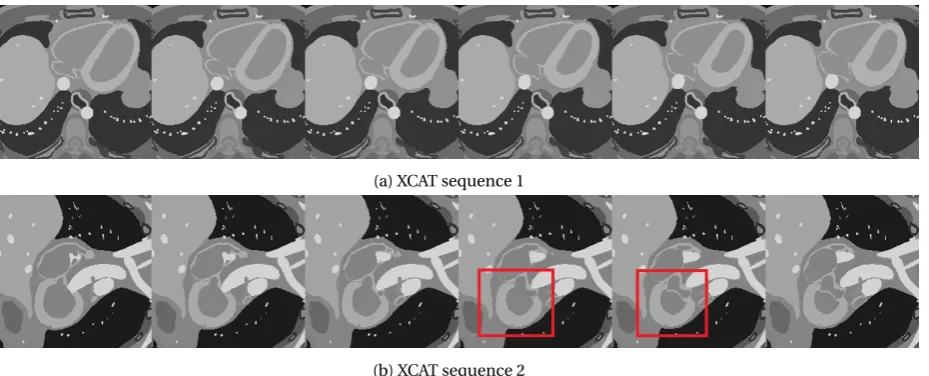
In this thesis a joint reconstruction and motion estimation framework is developed for dynamic MRI to explic-itly model the temporal coherence in a sequence. To address the challenging optimization of such a model, we will develop an algorithm related to recently developed nonconvex optimization algorithms. To evaluate the performance of the joint model for different optimization methods we develop synthetic datasets. These datasets are based on the MPI dataset [37] from computer vision, which has a ground truth for the flow field and the XCAT phantom [49], which is used for medical image reconstruction evaluation and made available by the radiotherapy group of the UMC Utrecht. Finally the model is applied to experimental medical data, also made available by the radiotherapy group of the UMC Utrecht, to show its potential for real word scenarios.

Structure

(9)

Chapter 2 Model for joint reconstruction and motion

estimation

In this thesis we consider the following general variational model for joint reconstruction and motion estima-tion:

min u,v

ZT

0

G(u)+J(Au)+F(Bv)+M(u,v)dt, (2.1) wereG(u) represents the data-fidelity for the image sequenceu, which penalizes differences between the im-age sequence and the observed data. Since the problem of MRI reconstruction is ill-posed due to noise and subsampling we need to use regularization. J(Au) represents the regularization term for theuand is used to incorporate a priori knowledge we have about the image. The problem of motion estimation is also ill-posed and hence we incorporate also a regularizer for the flow fieldv, namelyF(B v). The motion model is here rep-resented byM(u,v) which couples the image sequence and the flow field.

In this chapter we will define specific choices forG(u), J(Au),F(Bv) andM(u,v) and discuss related previ-ous work.

2.1 Data fidelity for MRI Reconstruction

Define the measurements from the MRI scanner as: f :Σ→C, withΣthek-space. As explained in the intro-duction, the signalf received during data acquistion is the Fourier transform of the image. Following [23] we assume that the phase of the received signal by the MRI scanner is negligibly small and henceu_∈_R2_{. Define:} u:Ω→R, whereΩ⊂R2.

Since the Fourier transform acts on complex valued images,u:Ω_→C, we define the operator Re(_·) as fol-lows:

Re :C_→R, Re(x₊i y)₌x, Re∗:R→C, Re∗(x)=x+i0.

Since we will use subsampling to reduce measurement time, we defineP(·) as the subsampling operator:

P(x) :=

(

1 ifx_∈π(Σ)

0 else ,

(10)

Definition 1: Forward operator static MRI reconstruction

Define the operator F:X(Ω)→Y(Σ), withΣthe k-space as F(u)₌P(F(Re∗(u))),

with Re∗the adjoint of the operator Re,F(·)the Fourier Transform, P(·)the subsampling operator and X and Y the appropriate function spaces. Then the adjoint operator is:

F∗=Re(F−1(P(f))),

with f _∈_Σ.

Since we want to reconstruct dynamic sequences we have to define the forward operator for dynamic MRI. The image sequenceu(·,t) is a function of the space-time domainΩ×[0,T] toR×[0,T]. Now we can define:

Definition 2: Forward operator dynamic MRI reconstruction

Define the operator F:X(Ω×[0,T])→Y(Σ×[0,T]), withΣ×[0,T]the k-t -space as F(u(_·,t))₌P(F(Re∗(u(_·,t)))),

with P(·,t)subsampling operator extended to:

P(x,t) :=

(

1 if x_∈π(Σ,t)

0 else ,

withπ(Σ,t)the set of coordinates in k-t space that are sampled.F(·,t)the Fourier Transform and Re∗(·,t)

as defined before, for each t . X and Y are the appropriate function spaces.

So for eacht∈[0,T], the forward operator for dynamic MRI reconstruction is the forward operator for static MRI reconstruction. Hence frame-by-frame reconstruction is possible. Note that time is defined equally in both the image and measurement domain, so at each point in time we have a set of measurements.

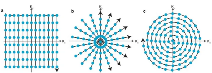
In practice,π(Σ,t) at timet will follow a pattern. Widely used are Cartesian, radial and spiral patterns: see Figure 2.1 for an example. Most simple is Cartesian sampling, where there is only subsampling in the phase-encoding direction. The classical Fourier transform can be used to model Cartesian subsampling. For radial and spiral subsampling the non-uniform Fourier transform must be applied or first a regridding procedure must be applied. As the optimal subsampling pattern is out of the scope of this thesis, only Cartesian subsam-pling is considered for simplicity.

As mentioned by [48], the noise present in MRI measurements is Gaussian, so we use theL2(Ω) norm for the data-fidelity. The data-fidelity for MRI reconstruction becomes:

[image:10.595.119.484.592.719.2]

G(u(·,t))= kF(u(·,t)−f(·,t)k22.

(11)

2.2 Regularizer for MRI reconstruction

Due to the presence of noise and subsampling, reconstructing an MR image is ill-posed and hence we have to add regularization for the image sequenceu(·,t). In this section different regularizers will be discussed and we will define the regularizerJ(Au) in (2.1).

2.2.1 Compressed sensing

In image processing it is well known that images are sparse in some transforms. So if we transform an image with an appropriate transform we only need a small part of that data to reconstruct the full image. This is the idea behind compressed sensing, which was applied to MRI by Lustiget al.in [36]. To apply compressed sensing there are three requirements:

1. The image is sparse in some transformation.

In [36] the finite difference, wavelet en discrete cosine transform are used. 2. The artefacts due to subsampling are incoherent (noise-like) in this transform.

To fulfill this requirement random subsampling in the phase encoding direction (y) is used in [36]. 3. We can reconstruct by enforcing both the sparsity and data consistency with the acquired data.

So the problem that is solved in compressed sensing for MRI can be written as: min

u kΦ(u)k1, s.t. _kF(u)₋f_k2₂_<ε,

(2.2)

wereΦis the sparsifying transform.Here we will use the Daubechies wavelet as the sparsifying transform. We can rewrite problem 2.2 to an unconstrained optimization problem by introducing the constantαand moving the constraint to the objective:

min u

λ

2kF(u(·,t))−f(·,t)k 2

2+αkΦ(u(·,t))k1, where enforcing sparsity in theΦ(u) transform is used as a regularizer.

2.2.2 TV and TGV regularization for MRI

A famous variational model is the ROF-model [47], were anL2data-fidelity is combined with total variation (TV) regularization. Total variation of a function is defined as:

T V(u) :₌ sup g∈C∞

0 (Ω;Rd),kgk∞≤1 Z

Ωu∇ ·gdx.

Depending on the inner norm chosen forkgk∞we get either isotropic total variation, which favours rounded

(12)

To overcome this, Knollet al.[29] propose total generalized variation (TGV) for MRI reconstruction. In their work they show that using the second order total generalized variation as regularizer gives better reconstruc-tions for static MRI, compared to using TV-regularization. Second order TGV prefers constant and piecewise linear images. As the TGV is also a semi-norm of a Banach space, the analysis and optimization is comparable to the using total variation. The second order total generalized variation is defined as:

TGV2_α(u) :₌min u1 α1

Z

Ω|∇u−u1|dx+α0 Z

Ω|E(u1)|dx, withE(u1)=1₂(∇u1+ ∇uT₁).

According to [29], usingα0=2α1offers in practice good results, so using TGV-regularization instead of TV-regularization does for this parameter choice not result in more parameters to be tuned.

2.2.3 Low-rank plus sparse decomposition

In [40], Otazoet al.propose a low-rank plus sparse matrix decomposition as regularization for dynamic MRI reconstruction. The decomposition is performed on the space-time matrixUwhose columns contain the im-age at each time step.

If we can decompose this space-time matrix in a part that represents the static background and a part that represents the dynamic foreground, then the static background will be a matrix of low column rank as each column is nearly the same. The matrix containing the dynamic information will now be defined as the sparse representation of this matrix using a temporal transform. The minimization problem for low-rank plus sparse decomposition is:

min

L,S λLkLk∗+λSkT Sk1+ 1

2kF(L+S)−fk 2 2.

withFthe forward operator for MRI reconstruction,f the measurements andLthe low-rank space-time ma-trix modeling the static background.k · k∗is the nuclear norm, defined as:

kA_k_∗₌trace³pA∗_A´_.

Sis the space-time matrix modeling the dynamic foreground which is sparse in the transformT(_·).

2.2.4 Infimal convolution of total generalized variation functionals for dynamic MRI

(ICTGV)

Another possible regularizer is given by Schloeglet al.[48]. They argue that in practise it is not always feasible to decompose the image sequence in a static background and dynamic foreground as proposed by [40]. To generalize this idea they propose a model that optimally balances between strong spatial or strong temporal regularization of the sequence. This is done via infimal convolution of total generalized variation functionals (ICTGV).

The ICTGV is defined as:

ICTGV2_β_,_γ=min

v βTGV 2

β1(u−v)+γTGV 2 β2(v),

(13)

2.2.5 Overview of regularizers for MRI reconstruction

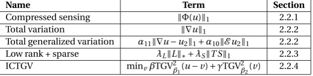
The options treated in this section are summarized in table 2.1. Since we want to incorporate the temporal coherence via joint reconstruction and motion estimation we will not use the low-rank plus sparse and ICTGV regularization since they also model temporal coherence.

In [18] TV-regularization was used as regularizer for the image sequence. We extend the regularization by adding the compressed sensing regularization term to obtain a suitable model for MRI reconstruction. So we defineJ(Au) as:

J(Au) :₌α1k∇u(·,t)k1+α2kΦ(u(·,t)k1.

Name Term Section

Compressed sensing kΦ(u)k1 2.2.1

Total variation _k∇u_k1 2.2.2

Total generalized variation α11k∇u−u2k1+α10kEu2k1 2.2.2 Low rank + sparse λLkL_k_∗₊_λ_SkT S_k1 2.2.3 ICTGV minvβTGV2_β₁(u−v)+γTGV2_β₂(v) 2.2.4 Table 2.1: Different choices for regularizationJ(Au) of MRI reconstruction

2.3 Model for motion estimation

In this section the goal is to define the motion modelM(u,v). As mentioned in the introduction we will use optical flow to model the motion. Optical flow is defined as the apparant motion between two consecutive frames, see Figure 2.2.

A common assumption is that the intensity of the image stays constant over time, which means that after

δtthe following equation must be satisfied:

u(x,t)=u(x+v(x,t),t+δt), (2.3) withv(x,t) :Ω_×[0,T]_→R2_×[0,T] the flow field which represents the displacement. If the movement is small, the linearization of 2.3 will lead to the well-known optical flow constraint (OFC):

∂tu(x,t)+ ∇u(x,t)·v(x,t)=0, which holds pointwise for each (x,t).

Now we define:

M(u,v) :=γ

pk∂tu(·,t)+ ∇u(·,t)·v(·,t)k

p

p, (2.4)

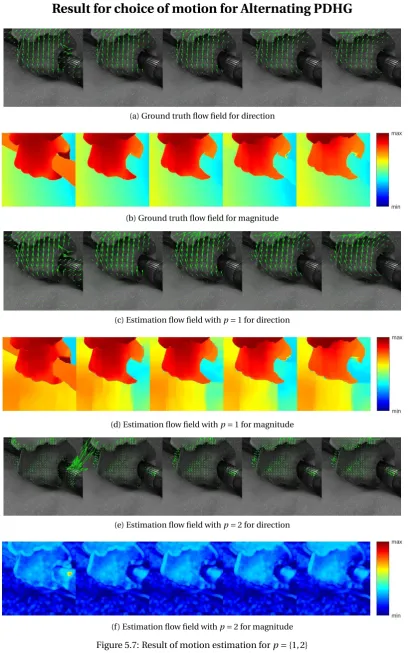
withp∈{1, 2}. Choosingp=1 will result in a motion model that is more robust to noise as presented by [3]. Choosingp=2 result in a smooth functionalM(u,v) which is favorable from an optimization point of view. Therefore both choices are considered.

[image:13.595.141.457.203.280.2]

(a) Image att (b) Image att+δt (c) Flow field

(14)

The optical flow constraint assumes that over time the intensity in an image remains constant when following the motion, however in changing illumination conditions this condition is violated. Another assumption is that the movement between two frames is small compared to the pixel size, this assumption is in practice also easily violated. In this thesis we will use the model for motion estimation as presented above. In the remainder of this section we will give a summary of related motion estimation models.

Mass preservation

A more general approach is to assume that the total brightness in the image is constant over time. This will lead to the mass preservation constraint.

∂tu+ ∇(uv)=0.

This constraint is known in literature as the continuity equation. A derivation can be found in [18]. Note that these two constraints intersect when∇ ·v=0. So for divergence-free flow fields both the optical flow and the mass preservation constraints are satisfied at the same time. A divergence-free flow fields corresponds to an incompressible flow, so there are no sources or sinks.

Preservation of intensity derivatives

Even more general is the assumption of preservation of the derivatives of intensity, as presented in [11]. Due to illumination changes the optical flow constraint will not hold, however the gradient of the image will remain constant in the case of constant illumination changes.

Non-linear motion model

Recall that the linearization of (2.3) holds if the movement is relatively small. However in many real life ap-plications this is not the case and hence the obtained model for the motion is not valid. To deal with this in [25], [42] and [50] variational models with non-linear models for motion estimation via optical flow are pre-sented. However these models are more difficult from a computational point of view.

In [42] the motion is estimated with a course-to-fine scheme. The main idea behind such a scheme is to create a series of down-sampled images. We start by estimating the motion on the most coarse scale, where the motion is now relatively small. Then we go step-by-step to a more fine scale, using the flow field estimated in the previous scale to get the flow field on the current scale.

In [50] an alternative to a coarse-to-fine scheme is given. They introduce an auxiliary flow fieldwto decouple the data-fidelity and regularization, which simplifies the optimization.

Image registration

A different way of modelling motion estimation is image registration. Here the goal is to find a deformation

y:Ω_→Rdsuch that for two given imagesI1andI2,I2(y) approximatesI1as good as possible. So instead of a flow field we are looking for a deformation to explain the movement between two images.

Time-dependent motion model

A possible extension to the motion model presented here is to make the motion estimation time dependent. Optical flow describes how to go from one to the next consecutive frame in time. However over time the flow field should also satisfy some regularity constraints. For example one could assume that the flow field should change smoothly over time. Incorporating temporal coherence of the flow fields can be modelled via optimal transport as presented in [11] or via optimal control optical flow [9], [16].

2.4 Regularizer for motion estimation

(15)

[image:15.595.139.455.71.192.2]

Figure 2.3: Illustration of the aperture problem from [25]. The different type of motions in the aperture are not distinguishable.

The variational model of Horn and Schunck for determining optical flow has the following form:

min

v

ZT

0 1

2k∂tu(·,t)+ ∇u(·,t)·v(·,t)k 2 2+

β

2k∇v(·,t)k 2 2dt.

Using_k∇v(_·,t)_k2₂as a regularizer will result in smooth flow fields. This is a reasonable assumption since an object in a sequence stays connected over time and therefore will have a smooth flow field.

However in the case of multiple moving objects the assumption of a smooth velocity field is not realistic. It would be desirable to allow discontinuites in the flow field on the edges of the objects. Papenberg, Weickertet al.[42] proposed TV-regularization to overcome this problem. TV-regularization results in constant areas and discontinuities along edges of objects in the flow field.

In the data considered here there is often a static background and a moving foreground, therefore smooth flow fields are not realistic and we define the following regularization for the flow fieldv:

F(Bv) := k∇v(·,t)k1. (2.5) There are many more possible regularizers, e.g. in [52] PDE-based regularizers are discussed. There regulariz-ers fall into two categories, namely image- or flow-driven.

Image-driven regularizers use the idea that motion boundaries are a subset of the image boundaries. So one way to combine smooth flow fields within an object and sharp edges on the motion boundaries, is to add a function to the regularizer that is small at the image boundaries. A risk of this approach is to get an overseg-mented flow field for textured objects.

Another type of regularizers are flow-driven. They also make us of a function that is small at the edges, but now at the edges of the flow field instead of the edges of the image. This will prevent oversegmentation but will have less sharp edges. So the choice depends strongly on the type of problem at hand.

(16)

Chapter 3 Analysis of joint MRI reconstruction and

motion estimation model

In the previous chapter we defined all the main ingredients of our joint model. In the chapter this model will be analyzed. First the model will be transferred to a more general function spaces setting, in which existence of a global minimizer is proved. We will also show that the joint model is not convex in both variablesuandv.. Finally the Kurdyka-Lojasiewicz property is treated and we prove that our model satisfies this property, which is a key element for convergence analysis in nonconvex optimization.

3.1 Variational model

Our aim is to minimize the following variational model for joint MRI reconstruction and motion estimation.

Joint reconstruction and motion estimation model

min u,v

ZT

0

G(u)₊J(Au)₊F(Bv)₊M(u,v)dt. (3.1)

with:

G(u)₌λ

2kF(u(·,t))−f(·,t)k 2 2, J(Au)=α1k∇u(·,t)k1+α2kΦ(u(·,t))k1, F(Bv)₌β_k∇v(_·,t)_k1,

M(u,v)=γ

pk∂tu(·,t)+ ∇u(·,t)·v(·,t)k

p

p p∈{1, 2}.

with image sequenceu(x,t) :Ω_×[0,T]_→Rand velocity fieldv(x,t)₌(v1,v2) :Ω×[0,T]→R2forΩ∈Rd. Recall that F(·,t) is the forward operator for dynamic MRI, f(·,t)∈Σ×[0,T] are the (subsampled) measurements ink-tspace andΦ(·,t) is the wavelet transform.

Remark:F(_·,t)₌P(F(Re∗₍_u₍_·_,_t_{)))) is time-dependent, as}_P₍_·_{) is dependent on time, but the operator works}

(17)

3.2 Existence of minimizer

In this section we will prove the existence of a global minimizer. This proof is an extension of the proof given in [12]. First we will state the important definitions and theorems needed for the proof. Then we will give an outline of the proof given in [12] and state what is left to prove for the model presented here. We conclude this section by proving this.

3.2.1 Definitions and theorems

To prove the existence of a minimizer we will use the fundamental theorem of optimization:

Theorem 1: Fundamental theorem of optimization

Let(U,τ)be a metric space and J:U_→R_{∪ ∞}a functional on U . Moreover let J be lower semi-continuous and coercive. Then there exists a minimizeru¯_∈U such that:

J( ¯u)₌inf u∈UJ(u).

To use this theorem we need lower semicontinuity and coercivity, which is defined as follows.

Definition 4: lower semicontinuity

In U a Banach space with topologyτ, functional J(U,τ)_→R¯ is called lower semicontinuous at u if: J(u)≤lim inf_kJ(uk) as k_{→ ∞},∀uk→u in topologyτ.

Definition 5: coercivity

Let(U,τ)we a topological space and J:U→R∪ ∞a functional on U . We call J coercive if it has compact sub-level sets. This means there exists anα∈Rsuch that the set:

S(α) :₌{u_∈U_|J(u)_≤α}

is not empty and compact in_τ.

To prove coercivity often the theorem of Banach-Alaoglu is employed.

Theorem 2: Banach-Alaoglu

Let U be the dual of a Banach space and C>0. Then the set:

{u_∈U:_ku_kU_≤C}

is compact in the weak-∗topology.

3.2.2 Outline of the proof

In [12] the existence of a minimizer is proved for the following joint model:

ZT 0

1

2kK u(·,t)−f(·,t)k 2

2+αk∇u(·,t)k1+βkv(·,t)k1dt s.t._∂tu(·,t)+ ∇u(·,t)·v=0 inD0(Ω×[0,T]),

(3.2)

There are two differences between this joint model and our joint model (3.1):

• In (3.2) the motion model appears as a constraint which must be satisfied in the distributional sense. This is equivalent to making (3.2) an unconstraint minimization problem using aLppenalty term, with

p∈{1, 2}, so this is equivalent to our motion model in (3.1).

• In (3.1) we have an additional regularization term foru. We will call this term:

JC S:=

ZT

(18)

To prove existence of a minimizer for (3.2) the following steps must be followed: 1. Transferring (3.2) to the right function space setting,

2. Checking all assumptions made by [12] for (3.2), 3. Proving lower semicontinuitiy for (3.2),

4. Proving the coercivity of (3.2) using the theorem of Banach-Alaoglu, 5. Proving convergence of the constraint in (3.2),

then from the fundamental theorem of optimization the existence of a minimizer will follow. In the following section we will take these steps to prove existence of a minimizer.

3.2.3 Proof of existence of a minimizer

1. Transferring(3.1)to the right function space setting

Following [12] we can write:

J(u,v)₌min u,v

Z T

0

λ

2kF(·,t)u(·,t)−f(·,t)k 2 2dt+α1

Z T

0 |∇

u(_·,t)_|p_BVdt₊α2

ZT

0 kΦ

(u(_·,t))_k1dt

+β

ZT

0 |∇x

v(_·,t)_|_BVq dt,

s.t.∂tu(·,t)+ ∇u(·,t)·v(·,t)=0 inD0(Ω×[0,T]). with (u,v) in the set:

n

(u,v) :u_∈Lpˆ(0,T:BV(Ω)),v_∈Lq(0,T;BV(Ω)),_{∇ ·}v_∈Lp∗s(0,T:L2k(Ω)),∂tu+ ∇u·v=0

o

, fors_>1,k_>2 andp∗_{such that}1

p+ 1

p∗=1 and ˆp=min{p, 2}.

2. Checking assumptions

In the proof of [12] four assumptions are made: 1. The dataf is affected by additive Gaussian noise. 2. Finite speed of the velocity field, i.e.:

kv_k_∞_≤cv< ∞ a.e.Ω×[0,T]. 3. Bound on the compressibility ofv, which means bounding∇ ·v. 4. ForF(1t)6=0,∀t∈[0,T], with1tthe indicator function.

All four assumptions follow naturally for the model presented here. As mentioned in chapter 2, noise that affect MRI data is indeed Gaussian noise, hence the choice for anL2data-fidelity term. We assume that the object that is scanned will remain visible during data acquisition, thus the velocity field is bounded by the res-olution of the resulting image. The image is defined on a bounded subsetΩ∈Rd. Hence we have indeed finite speed.

Bounding compressiblity relates to bounding the sources and sinks in the flow field, which is reasonable. Fi-nally for the forward operator it must hold thatF(1t)6=0,∀t_∈[0,T]. So for1t, with arbitraryt_∈[0,T] we get:

Re∗(1t)=1t+0i, since the indicator function is a real function,

(19)

withδ(Σ) the Dirac delta function on thek-spaceΣ. The Dirac delta function is defined as:

δ(x)=

(

∞ ifx₌0 0 else

Now forP(δ(Ω)) att∈[0,T] to be nonzero, 0∈π(Σ) at timet. We will see later this will always be the case for the subsampling pattern considered in this thesis, as most of the energy of the image in the Fourier domain is in the center.

3. Lower semicontinuity

In [12] the lower semicontinuity of (3.2) is proved. The term JC Sis an affine norm of the formkΦ(u)k1and hence lower semicontinuous. Since the sum of lower semicontinuous functionals is also lower semicontinu-ous, we proved lower semicontinuity for (3.1).

4. Coercivity

In [12] coercivity is proved for (3.2) with the additional remark that the functional (3.2) is coercive for any regularizerJ(u(·,t)) for which holds:

R(u(·,t))≥ |u(·,t)|pBV, so if we can prove this inequality, coercivity will follow.

We have that:

R(u_·,t) := |u(·,t)|pBV+ kΦ(u(·,t))k1, so we must prove

kΦ(u(·,t))k1=

Z T

0 |Φ

(u(·,t))|dt≥0,

which holds by the definition of a norm, which concludes the prove for coercivity.

5. Convergence of the constraint

This is proved in [12] and hold also for our model (3.1).

Now the existence of a minimizer follows from the fundamental theorem of optimization. ä As we will see in the next section, the functional (3.1) is nonconvex foruandv, so we are not able to prove uniqueness of the minimizer.

3.3 Convexity

ForJ(u,v) (3.1) to be a convex functional the following definition from [46] must hold:

Definition 6: Convex functional

Let U be a Banach space,Ω_⊂U a convex subset and J:Ω_→R_∪∞a functional. J is convex if the inequality: J(αu1+(1−α)u2)≤αJ(u1)+(1−α)J(u2) (3.3) holds for all u,v_∈Ωandα_∈[0, 1]. J is strictly convex if (3.3)holds with strict inequality andα_∈(0, 1).

Following [46], we know that:

Lemma 1: Convex functionals

The following holds:

(20)

3. For two convex functions u1, u2it holds: u1+u2is convex. 4. The integral of the sum of two functions u1, u2is convex. Proof:The proof of 1.1,1.2 and 1.3 can be found in [46]

For 1.4:

J(αu1+(1−α)u2)=

Z T 0 α

u1+(1−α)u2dt

=

Z T 0 α

u1dt+

Z T 0

(1−α)u2dt

=α

Z T 0

u1dt+(1−α)

Z T 0

u2dt =αJ(u1)+(1−α)J(u2).

ä

Using lemma 1.3 and 1.4 we can analyze the convexity of (3.1) term by term. The data-fidelity term foru, the regularization term foruand the regularization term forvare all norms or affine norms. However:

JOF C=∂tu(·,t)+ ∇u(·,t)·v(x,t) (3.4) this is the only term in (3.1) wereuandvare coupled. As it turns out this term is not jointly convex foruandv.

Theorem 4: Nonconvexity joint model

The term(3.4)is not jointly convex for u andv. As a consequence the model(3.1)is not jointly convex. Proof:

ForJOF C to be jointly convex foruandvthe following must hold:

JOF C(αu+(1−α)u,αv+(1−α)v)≤αJOF C(u,v)+(1−α)JOF C(u,v), for allu_∈Lp(0,T;BV(Ω)),v_∈Lq(0,T;BV(Ω)) andα_∈[0, 1].

Now:

JOF C(αu1+(1−α)u2,αv1+(1−αv2))=α∂tu1+(1−α)∂tu2+α2∇xu1·v1+(1−α)2v2 +α(1−α)(∇xu1·v2+ ∇xu2·v1),

(3.5)

αJOF C(u1,v1)+(1−α)JOF C(u2,v2)=α∂tu1+(1−α)∂tu2+α∇xu1·v1+(1−α)v2. (3.6) ForJOF C to be convex, (3.5)≤(3.6) must hold. Forα∈[0, 1] the following holds:

α2 ≤α, (1−α)2≤(1−α). Hence we must prove:

α(1−α)(∇xu1·v2+ ∇xu2·v1)≤0,

for allα_∈[0, 1] andu_∈Lp(0,T;BV(Ω)) andv_∈Lq(0,T;BV(Ω)). Forα₌0 orα₌1 this inequality is satisfied, however forα_∈(0, 1), this is not the case. Take for examplev1=[1, 0] andv2=[0, 1] for allx∈Ωand allt∈[0, 1] andu1:=xandu2:=y, wereΩ∈R2+. Then we get for everyx,y,t∈Q:

α(1₋α)

µ £

1 0¤

·

1 0

¸

+£0 1¤

·

0 1

¸¶

=2α(1₋α),

(21)

3.3.1 Biconvexity

Although (3.1) is not jointly convex, the energy is biconvex. Biconvexity is defined as follows.

Definition 7: Biconvex sets and functionals

Let U,V be a Banach space,_Ω_⊆U_×V a biconvex subset and J:_Ω_→_R_{∪ ∞}a functional. A set B_⊂U_×V is a biconvex subset on U_×V if:

1. for every u∈U and fixedvˆ∈V , Bvˆis a convex set. 2. for every v_∈V and fixeduˆ_∈U , Buˆis a convex set. A functional J is biconvex if:

1. ∀u∈U and fixedvˆ∈V , J(u, ˆv)is a convex functional. 2. _∀v_∈V and fixeduˆ_∈U , J( ˆu,v)is a convex functional.

Now we can prove the biconvexity of the joint model.

Theorem 5: Biconvexity of joint model

The model (3.1) is biconvex.

Proof:For

JOF C=∂tu(·,t)+ ∇u(·,t)·v(x,t) with fixed ˆuand respectively ˆv, we can write:

JOF C( ˆu,v)=Auv−fu

JOF C(u, ˆv)=Avu

withAu= ∇u,fu=∂tuandAv=[∂t+vx∂x+vy∂y]. Using Lemma 1.1 and 1.2,JOF Cis biconvex. ä

3.4 The Kurdyka-Lojasiewicz property

Since our model for joint reconstruction and motion estimation is not jointly convex for both variablesuand

vthe optimization is challenging. The key property to prove convergence in nonconvex optimization is the Kurdyka-Lojasiewicz property. In this section this property is stated and proved for the discretization of the functional (3.1).

The Kurdyka-Lojasiewicz (KL) property was first introduced by Lojasiewicz [32] for real analytic functions. Kurdyka [30] extended the property to functions definable on the minimalo-structure. Finally Bolteet al.[7] extended the KL property for nonsmooth subanalytic functions.

For real analytic functions we can define the KL-property as follows.

Definition 8: KL-property for real anaytic functions [32]

A functionψ(x)satisfies the KL property at pointx¯_∈Dom(∂ψ)if in a neighborhood U ofx, there exists a¯

functionφ(s)₌c s1−θfor some c_>0andθ_∈[0, 1)such that the KL inequality holds:

φ0₍_|_ψ₍_x₎₋_ψ_{( ¯}_x₎_|_)dist(0,_∂ψ₍_x₎₎_≥_{1 for any}_x_∈_U_∩_dom(_∂ψ_{) and}_ψ₍_x₎₆₌_ψ_{( ¯}_x_). _(3.7)

wheredist(x,S) :₌infy{ky−xk|y∈S}.

This definition can be extended for general proper lower semicontinuous functions. Takeη_∈(0,_+∞]. Take

φ: [0,η)_→R+_{a concave continuous function such that:}

1. φ(0)₌0,

(22)

Now we can state:

Definition 9: KL-property for proper lower semicontinuous functions [7]

Letψ(x) :Rd →(−∞,+∞]be proper and lower semicontinuous. The functionψhas the KL property at

¯

x∈dom(∂ψ)if there exist aηas defined before and a neighborhood U ofx and a function¯ φas defined before, such that for all:

x∈U∩[ψ( ¯x)<ψ(x)<ψ(x)+η]

the following inequality holds:

φ0₍_ψ₍_x₎₋_ψ_{( ¯}_x₎₎_dist_(0,_∂ψ₍_x₎₎_≥₁ _(3.8)

We say that a functionψhas the KL-property or is a KL-function if it satisfies definition 6 or 7 at each point of dom(_∂ψ).

3.4.1 KL-property for a two-dimensional problem

To get a better intuition for the KL-property we will consider the following two-dimensional problem: min

(x,y)∈R2ψ(x,y)=(x y−1)

2_. _(3.9)

This function is nonconvex in both (x,y), but convex for fixedxory, hence it is biconvex. We will analyze the KL-property for this function. Note that this is a polynomial function and hence real analytic, so we can use definition 8. The critical points of (3.9) are given by:

∇ψ=£

2y(x y₋1) 2x(x y₋1)¤

, soψ(x,y) is minimal fory₌1_x.

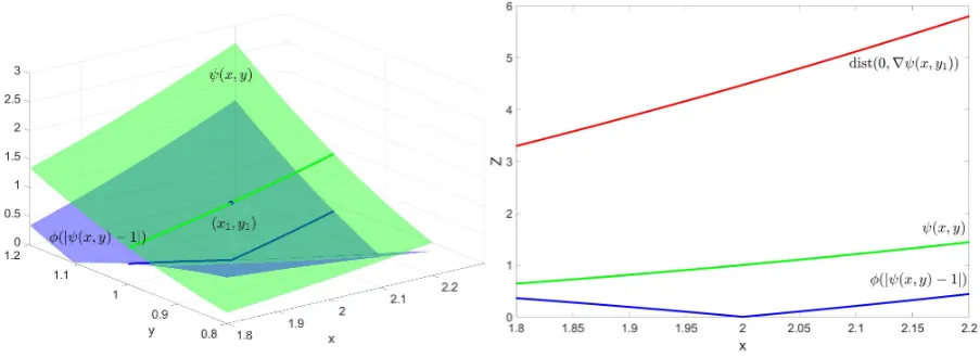
First consider (x1,y1) for which holdsy16=_x1₁. This is a noncritical point, which makes it easy to find a neigh-borhoodU1were dist(0,∇ψ(x) is not close to zero. Take for example (x1,y1)=(2, 1), withψ(2, 1)=1. Then we can takec₌1 andθ₌0, which givesφ₌s, soφ0₌_{1. In figure 3.1a we see in green}_ψ₍_x_,_y_{) in the neighborhood}

U1and in blueφ(|ψ(x,y)−1|). In figure 3.1b we see in red dist(0,∇ψ(x,y1), for the cross-section (x,y1) which is clearly greater than one and hence we fulfill the KL-inequality (3.7).

Near a critical point (x0,y0) for which holds y0= _x1₀. dist(0,∇ψ(x,y) will become close to zero in a neigh-borhoodU0. To fulfill the KL-property we must chooseφsuch that the reparametrizationφ(|ψ(x)|) issharp enough. Sharpness is important since the derivative ofφtimes the small distance between zero and the gra-dients ofψmust be greater or equal to one. Take for example (1, 1), wereψ(1, 1)=0 and chooseφ=2s0.5. In figure 3.2a we see in greenψ(x,y) near (1, 1) and in blueφ(|ψ(x,y)|), which is indeed sharper. In figure 3.2b, we see again in red dist(0,∇ψ(x,y) aty=1 nearx=1 and we see that this distance is smaller than one. In yellow we see the KL-inequality, which is fory=1 nearx=1, greater than one.

[image:22.595.77.529.538.703.2]

(a) Plot ofφ(|ψ(x,y)|) near (2, 1), withφ=s (b) cross-section aty=1 aroundx=2

(23)

[image:23.595.80.537.70.257.2]

(a) Plot ofφ(|ψ(x,y)|) andψ(x,y) near (1, 1) (b) cross-section aty=1 aroundx=1

Figure 3.2

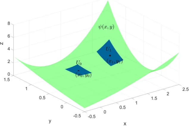
From this example we see that it is easy to establish the KL-property near non-critical points. Near critical points we must chooseφsuch that the reparametrization is sharp enough to compensate for the small gradi-ents such that the KL-property is satisfied. In figure 3.3 a plot ofψ(x,y) is shown with both neighborhoodsU1 andU0. Here we clearly see that near the non-critical point, the function is quite steep and near the critical point it is not. To prove convergence to a minimum for a nonconvex problem, the KL-inequality ((3.7),(3.8)) will be used to obtain a bound for the sequence generated by the algorithm.

Figure 3.3: Plot ofψ(x,y) with points (x1,y1) and (x0,y0) and their neighborhoodsU1andU0.

3.4.2 KL-property for joint model

To make use of algorithms for optimization of nonconvex functions, we need to prove that the discretization of the model for joint reconstruction and motion estimation is a KL-function.

[image:23.595.142.460.402.613.2]

(24)

so here we only state the resulting function:

min

u∈RN×t_,_v_∈_RM×tJ(u,v)=

T

X

t=0

λ

2kF ut−ftk 2

2+α1k∇utk +α2kΦutk1+ T−1

X

t=0

βk∇vtk1+γ

2k∂tut+ ∇ut·vtk 2

2. (3.10) To prove that this is a KL-function we will use the following lemma.

Lemma 2: KL functions

The following functions satisfy the KL-property:

1. Real analytic functions

2. Semialgebraic functions

3. Sum of real analytic and semialgebraic functions

Proof:For the proof of 1 see the work of Lojasiewicz [32], the proof of 2 follows from the work of Bolteet al.[7] since semialgebraic functions are subanalytic. For 3 we refer to [6] were they prove that the sum of two suban-alytic functions is subansuban-alytic. Note that both real ansuban-alytic and semialgebraic functions are subansuban-alytic [6]. ä First we will define what real analytic and semialgebraic functions are. The defintion can be found in [6].

Definition 10: real analytic and semialgebraic functions

A smooth functionφ(t)onRis analytic if:

Ã φk₍_t₎

k!

!1_k

is bounded for all k on any compact set D_⊂R. Forφ(x)onRncheck the analyticity ofφ(x₊t y)for any x,y_∈Rn.

A functionφis called semialgebraic if its graph:

{(x,φ(x)) :x_∈dom(φ)}

is a semialgebraic set. A set D_∈Rnis called semialgebraic if it can be represented as:

D= s

[

i=1 t

\

j=1

{x∈Rn:pi j(x)=0,qi j>0},

with pi j, qi jreal polynomial functions for i≤i≤s,1≤j≤t . Now we are ready to prove that (3.10) is a KL-function.

Theorem 6: Joint model is a KL-function

The function(3.10)is a KL-function. Proof:The proof consist of two parts:

1. Prove thatλ₂_kF ut−ftk2₂andγ₂k∂tut+ ∇ut·vtk2₂are real analytic functions for eacht∈[0,T]. 2. Prove thatα1k∇utk1,α2kΦutk1andβk∇vk1are semialgebraic functions for eacht∈[0,T]. If 1 and 2 hold then lemma 2.3 gives that (3.10) is a KL-function.

1. Note that both:

λ

2kF ut−ftk 2 2

γ

(25)

2. In [53] the authors show that thel1-norm is semialgebraic and conclude that any function of the form kAxk1is semialgebraic. So we find that:

k∇utk1 kΦutk1 k∇vtk1 are semialgebraic.

(26)

Chapter 4 Optimization

In this chapter the optimization of the joint model is explained. This is challenging since we established in the previous chapter that the functional is nonconvex. However the functional (3.1) is biconvex, so the first approach to optimize the functional is to alternate between the convex subproblems. This approach was used before in this context by [18]. In this chapter we will first treat splitting methods for convex optimization to solve the two convex subproblems. Subsequently we treat optimization methods for nonconvex functionals. Here the KL-property discussed in the previous chapter becomes really important. In the last section of the chapter we will compare both methods for a two-dimensional example. We start this chapter with by stating the discretization of the model.

4.1 Discretization

For the implementation of both algorithms the same discretization will be used. In this section the discretiza-tion is treated. We start by the discretizadiscretiza-tion of the image sequenceu(x,t), the measurements f(x,t) and the flow fieldv(x,t).

Discretization variables

The discrete version ofu(x,t)_∈_Ω_×[0,T] is defined as:

ui j t∈Rnx×ny×nt, withi∈{0 . . . ,nx},

j∈{0, ...,ny},

t_∈{0, . . . ,nt}.

If we refer touat timetfor alli,j, we will writeut. Forf ∈Σ×[0,T] the discretization is:

fi j t∈Cnx×ny×nt, withi∈

½

−1 2nx, . . . ,

1 2nx

¾

,

j∈

½

−1 2ny, . . . ,

1 2ny

¾

,

t∈{0, . . . ,nt}. Forv(x,t)∈Ω×[0,T] the discretization is:

vi j t∈Rnx×ny×nt−1×2, withi∈{0, . . . ,nx},

j_∈{0, . . . ,ny},

t∈{0, . . . ,nt−1}. additionally we will use the notationvi,j,t=

£

vxi,j,t vyi,j,t ¤

(27)

Remark:We used the same discretization of time for all three variables. This means thatvtat timetdescribes the deformation fromuttout+1. This means also thatftcontains all the measurements corresponding to the imageut. So we assumed that the time needed for each measurement is negligible small compared to the time between frames in the sequence.

Remark:We can reformulateu_∈_Rnx×ny×nt _to_u_∈RN_{, with}_N ₌_n

xnyntby vectorization, both notations will be used. The same holds forv_∈RMwithM₌nxny(nt−1)×2.

Discretization of operators

Next we have to discretize the operatorsF,_∇,Φand∂t and their adjoints. For the partial derivates, gradient and divergence we follow [18], and use forward differences for the spatial and temporal derivatives. However, for∂tu+ ∇u·v, for the discretization of∇central differences are used. This will result in a stable discretization in both variablesuandv. The definition of the forward, central and backward differences used can be found in appendix B.

For the operatorF=P(F(Re∗(·))), we discretize each component as follows. For the operator Re we can write now:

Re :CN_→RN, Re(x₊i y)₌x, Re∗:RN_→CN, Re∗(x)₌x₊i0.

For the Fourier transform we use its discrete counterpart applied for eacht∈[0,T]. We use the implementa-tion of the discrete Fourier transform in the AVIONIC toolbox [48]. Finally the subsampling operator can be discretized as follows:

P(x) :₌

(

1 ifx∈π(Σ)

0 else ,

withπ(Σ) the discretized set of spatial coordinates ink-space that are sampled.

For the wavelet transformΦwe use the discrete Daubechies wavelet with a filter of order four and a scal-ingsfactor of four. For the implementation we used Wavelab [19].

Now we can define the discretized version of (3.1):

min

u∈RN_,_v_∈_RMJ(u,v)=

T

X

t=0

λ

2kF ut−ftk 2

2+α1k∇utk +α2kΦutk1+ T−1

X

t=0

βk∇v_tk1+γ

2k∂tut+ ∇ut·vtk 2

2+χ+(ut). (4.1) wereχ₊(ut) is defined as:

χ+(ui,j,t) :=

(

0 ifui,j,t≥0 ∀i,j,t ∞ else,

to ensure thatumaps to positive values.

4.2 Splitting methods for convex optimization

Consider the following general convex minimization problem: min

x∈XT(x),

whereT(x) is a proper convex functional. The classical way to solve this problem is via the proximal point algorithm:

(28)

defined as follows:

x=(I+τ∂T)−1(y), =proxT_τ(y), =argmin

x

½

kx−yk2

2 +τT(x)

¾

.

(4.3)

Which could be interpreted as an approximation of a gradient descent step, where we seek a pointxin the domain of the functionalT(x) which is close to the previous pointywith step-sizeτ.

For some functionals the proximal map is easy and quick to determine. The key idea is to split the problem into functionals with easy to determine proximal maps and then apply those proximal maps subsequently to perform a full proximal step as defined in (4.2). One of the most well-known splitting methods is the Douglas-Rachford splitting [21], defined as:

xk+1₌(I₊τB)−1((I₊τA)−1(I₋τB)₊τB)(xk),

forT =A+B. Originally this method was defined for linear operators. However [31] extended the splitting method for general operators and as it turns out Douglas-Rachford splitting is a special case of the proximal point algorithm [22]. So iterating via Douglas-Rachford splitting will give the same solution as iterating 4.2. Now consider the following general convex minimization problem which can be written as:

min

x∈X F(K x)+G(x) (4.4)

whereKis a general bounded linear operator. This problem is called the primal problem. Using the definition of the convex conjugate of proper functionalJ:X_→R:

J∗(p) :=sup x∈X

©

〈p,x_〉X₋J(x)ª

forp_∈X∗

andJ∗∗₌_J_{, we can write:}

min

x∈XF(K x)+G(x)=minx∈X_psup_∈_X∗〈

p,K x〉X∗−F∗(p)+G(x)

=min x∈X _psup_∈_X∗〈

p,K x〉X∗−F∗(x)+G(x)

(4.5)

which is the saddle-point formulation for primal problem (4.4), withX∗_{the dual space of the Banach space}_X_.

Using the definition of the Gâteaux derivative, we can write down the optimality conditions: −KTp∈∂G(x)

K x_∈∂J∗(p). (4.6)

Another way of splitting the problem (4.4) is to decouple the problem using the substitutionK x=w: min

x,w F(w)+G(x) s.t. K x=w,

(4.7)

then we have the following Lagrangian:

L(x,w,p)=F(w)+G(x)+

p,K x−w®

with corresponding optimality conditions:

−K∗p∈∂G(x)

p_∈∂J(w)

(29)

which is clearly equivalent to (4.6). So the optimal solution to (4.4) is the same as for the decoupled problem (4.7). Solving (4.7) can be done by the Alternating Direction Method of Multipliers (ADMM) [10] , which turns out to be equivalent to applying the Douglas-Rachford splitting on the dual problem.

If we now apply an appropriate preconditioner using ADMM we arrive at the Primal-Dual Hybrid Gradient method of [15]. This algorithm is widely used and easy to implement. We will use this algorithm to solve the convex subproblems for the minimization the biconvex functional (3.1).

So if we can write the general convex minimization problem (4.4) as a saddle-point problem (4.5), then we can solve this via the following algorithm developed by Chambolle and Pock [15].

Algorithm 1: Primal-Dual Hybrid Gradient (PDHG)

• Initialize: Chooseτ,σ>0,θ∈[0, 1]. Set (x0_,_p0₎_∈_X_×_X∗_{and ¯}_x₌_x0_. • iterate fork_≥0xk,pkand ¯xkas follows:

    

pk+1

=(I₊σ∂F∗₎−1¡

pk₊σKx¯k¢

uk+1=(I+τ∂G)−1¡

xk−τK∗pk+1¢

¯

xk+1 =xk+1

+θ¡xk+1 −xk¢

.

(4.8)

Following [15], we will useθ₌1 in the remainder.

To conclude this section on splitting methods for convex optimization we want to point out another line of splitting methods. Namely the Proximal Forward-Backward(PFB) splitting, also known as Proximal Gradient Descent. This method can be applied to problems consisting of a smooth and non-smooth functional. We take then a forward or explicit step over the smooth part and a proximal or backward step on the non-smooth part. Hence we can write the update as follows:

(30)

4.3 Optimization method 1: Alternating PDHG

As established before the functional (3.1) is biconvex. So the first optimization approach as given in [18], is to alternate between the two convex subproblems. So the algorithm will consist of one outer loop, where we alternate between two inner loops. In the inner loops the subproblems are solved.

This gives optimization method 1 below. In the following sections we will derive the algorithms for the two inner loops based on PDHG, see algorithm 1.

Optimization method 1: Alternating PDHG

While error(un,vn)>tol, iterate forn≥0:

• Findun+1by solving thesubproblem for reconstruction:

un+1₌argmin u

J(u,vn),

=argmin u

Z T

0

λ

2kF(·,t)u(·,t)−f(·,t)k 2

2+α1k∇xu(·,t)k1+α2kΦ(u(·,t))k1 +γ

pk∂tu(·,t)+ ∇u(·,t)·v

n₍

·,t)kpp+χ+(u(·,t))dt.

(4.10)

• Findvn+1_{by solving the}_{subproblem for motion estimation}_:

vn+1=argmin

v

J(un+1,v), =argmin

v

ZT

0 βk∇

v(·,t)k1+γ pk∂tu

n+1₍

·,t)+ ∇un+1(·,t)·v(·,t)kppdt.

(4.11)

• error(u,v)₌|un+1−u₂_|n_Ω|+|_×_Tvn_|+1−vn|.

withp_∈{1, 2}. Next we will describe how to solve each subproblem.

Remark:Here we first optimize and then discretize.

4.3.1 Optimization of subproblem for reconstruction

We can rewrite the problem inu(4.10) as a saddle-point problem:

min

u p=[p1max,p2,p3,p4]

ZT

0 χ+

(u)+ 〈K u,p〉 − 1 2λkp1k

2

2− 〈p1,f〉 −α1δB(L∞)

µ_p

2

α1

¶

−α2δB(L∞)

µ_p

3

α2

¶

−F∗(p4)dt, were we defineF∗₍_p

4) as follows:

F∗(p4)=

( γδB(L∞)

³_p

4 γ

´

ifp₌1, 1

Joint reconstruction and motion estimation via nonconvex optimization for dynamic MRI