warwick.ac.uk/lib-publications
A Thesis Submitted for the Degree of PhD at the University of Warwick
Permanent WRAP URL:
http://wrap.warwick.ac.uk/88817
Copyright and reuse:
This thesis is made available online and is protected by original copyright. Please scroll down to view the document itself.
Please refer to the repository record for this item for information to help you to cite it. Our policy information is available from the repository home page.
Analysis, Improvements and
Applications
By
Jian Zhu
A thesis submitted for the Degree of
Doctor of Philosophy
Department of Engineering
University of Warwick
Contents
List of Figures ... VI
List of Tables ... XI
Acknowledgements ... XIV
Declarations ... XV
Summary ... XVI
Abbreviations ... XVII
Chapter 1 Introduction ... 1
1.1 Requirements of image coding ... 1
1.1. 1 Image and video compression ... 1
1.1.2 Lossless image coding ... 2
1.1.3 Lossy image coding ... 2
1.1.4 New features of image coding ... .3
1.2 Image coding methods ... 5
1.2.1 Statistical models ... 5
1.2.2 Physical models ... 8
1.3 Research objectives ... 8
Reference ... 10
Chapter 2 The Wavelet Transform ... 11
2.1 Two-channel filter banks ... 11
2.2 Biorthogonal filter banks ... 13
2.3 Perfect reconstruction FIR filter banks ... 15
2.4 Wavelet transform ... 17
2.4.2 Wavelet. ... 18
2.4.3 Wavelets from filter banks ... 18
2.4.4 Filter banks from wavelets ... 22
2.4.5 Summary and example ... 23
2.5 Multi-resolution decomposition ... 23
2.6 Two-dimensional wavelet transform ... 25
2.7 Edge extension ... 27
2.8 Arrangements of wavelet coefficients ... 30
2.9 Summary ... 34
Reference ... 36
Chapter 3 Statistical Properties of Wavelet Coefficients ... 37
3.1 Distribution of all wavelet coefficients ... .40
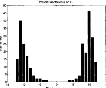
3.2 Distribution of wavelet coefficients on LL ... .43
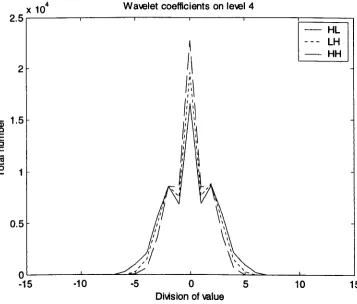
3.3 Distribution of wavelet coefficients on HL, LH and HH ... .46
3.4 Intra-subband correlation ... 54
3.5 Inter-subband correlation at same level ... 58
3.6 Inter-level correlation on HL, LH and HH ... 58
3.7 Summary ... 59
Reference ... 70
Chapter 4 SPIHT Image Coding ... 71
4.1 Organisation of wavelet coefficients ... 72
4.2 Successive approximation quantisation ... 75
4.3 Ordered bit-plane coding ... 76
4.4 Procedure of SPIHT coding ... 77
CONTENTS IV
4.6 Arithmetic coding ... 91
4.6.1 Arithmetic coding models ... 94
4.7 Summary ... 96
Reference ... 96
Chapter 5 Improvements to the SPIHT Algorithm ... 97
5.1 DC-level shifting ... 97
5.2 Introduce the virtual trees ... 98
5.3 Omit the predictable symbols ... 107
5.4 Offset the quantisation ... 109
5.5 Optimise the arithmetic coding ... 115
5.6 A simple example ... 117
5.7 Summary ... 126
Reference ... 127
Chapter 6 Pre-processing for SPIHT Coding ... 128
6.1 Speed up the judgement of significance of trees ... 128
6.2 Pre-processing for SPIHT ... 132
6.3 Summary ... 136
Chapter 7 Performance of SPIHT Image Coding ... 137
7.1 Implementation of the SPIHT algorithm ... 137
7.2 Performance of the SPIHT algorithm ... 141
7.3 Performance gain of the improvements to the SPIHT algorithm ... 146
7.3.1 DC-level shifting ... 146
7.3.2 Virtual trees ... 150
7.3.3 Omit predictable coding symbols ... 155
7.3.5 Pre-processing for lossy image coding ... 161
7.3.6 Arithmetic coding ... 164
7.3.7 Judgement of the significance oftrees ... 167
7.3.8 Overall rate-distortion performance gain ... 171
7.4 Speed ofthe SPIHT algorithm ... 181
7.5 Summary ... 184
Reference ... 185
Chapter 8 Lossless image coding using the SPIHT algorithm ... 186
8.1 Reversible integer-to-integer wavelet transforms ... 186
8.2 Performance evaluation of the integer wavelet transforms for the SPIHT algorithm ... 189
8.3 Content-based lossless image coding using the SPIHT algorithm ... 193
8.4 Summary ... 202
Reference ... 203
Chapter 9 Discussion and Conclusions ... 204
9.1 Summary and conclusions ... 204
9.2 Future work ... 209
Reference ... 211
List of Figures
Figure 1.1 Neighbours used for prediction in CALIC. ... 6
Figure 1.2 Transform coding system ... 6
Figure 2.1 Two-channel filter banks ... 11
Figure 2.2 Three-level octave decomposition ... 24
Figure 2.3 Three-level octave reconstruction ... 24
Figure 2.4 2D separable wavelet analysis ... 26
Figure 2.5 2D separable wavelet synthesis ... 26
Figure 2.6 Subbands of 3-scale wavelet transform ... 27
Figure 2.7 Periodic extension ... 28
Figure 2.8 Symmetric extension ... 29
Figure 2.9 Symmetric extension without overlapping ... 30
Figure 2.10 Down/up-sampling and edge extension in case of odd length input ... 31
Figure 2.11 Down/up-sampling and edge extension in case of even length input.. ... 32
Figure 2.12 Results of 3-scale wavelet transform, 50 x 37 image ... 33
Figure 2.13 Edge extension without overlapping in case of odd length input ... 34
Figure 3.1 Lena (512x512, 8bpp) ... 38
Figure 3.2 Subbands of 5-scale wavelet transform ... 39
Figure 3.3 Distribution of all wavelet coefficients of Lena (linear axis) ... .40
Figure 3.4 Distribution of all wavelet coefficients of Lena (log y-axis) ... .41
Figure 3.5 Distribution of all wavelet coefficients of Lena (non-linear x-axis) ... .42
Figure 3.6 Distribution of wavelet coefficients on LL of Lena ... 44
Figure 3.8 Distribution of wavelet coefficients on LL of Lena after DC-level shifting
... 45
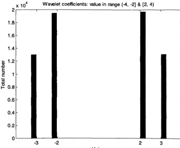
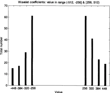
Figure 3.9 Distribution of wavelet coefficients on level 4 of Lena ... .47
Figure 3.10 Distribution of wavelet coefficients of Lena in division ±2 ... .48
Figure 3.11 Distribution of wavelet coefficients of Lena in division ±3 ... .48
Figure 3.12 Distribution of wavelet coefficients of Lena in division ±4 ... .49
Figure 3.13 Distribution of wavelet coefficients of Lena in division ±5 ... .49
Figure 3.14 Distribution of wavelet coefficients of Lena in division ±5 ... 50
Figure 3.15 Distribution of wavelet coefficients of Lena in division ±6 ... 50
Figure 3.16 Distribution of wavelet coefficients of Lena in division ±7 ... 51
Figure 3.17 Distribution of wavelet coefficients of Lena in division ±8 ... 51
Figure 3.18 Distribution of wavelet coefficients of Lena in division ±9 ... 52
Figure 3.19 Distribution of wavelet coefficients of Lena in division ± 10 ... 52
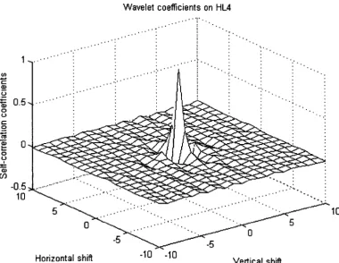
Figure 3.20 Intra-subband correlation of wavelet coefficients of Lena on HL4 ... 55
Figure 3.21 Intra-subband correlation of wavelet coefficients of Lena on LH4 ... 55
Figure 3.22 Intra-subband correlation of wavelet coefficients of Lena on HH4 ... 56
Figure 3.23 Intra-subband correlation of wavelet coefficients of Lena on HHO ... 56
Figure 3.24 Barbara ... ··· .. ··· .. ··· ... ···.··· .... ·· ... 60
Figure 3.25 Boats ... 61
Figure 3.26 Goldhill ... · .. · .... ·· .. ···· .. ·· .. ··· ... ··· ... 62
Figure 3.27 Mandrill ... ··· .. ··· .. ··· .... ··· .. · ... 63
Figure 3.28 Peppers ... ··· .. ··· ... 64
Figure 3.29 Zelda ... ··· .. ··· ... 65
Figure 3.30 Distribution of wavelet coefficients on LL ... 67
LIST OF FIGURES VIII
Figure 4.1 SPIHT image coding system ... 71
Figure 4.2 Correspondence of wavelet coefficients on different levels ... 73
Figure 4.3 Value of wavelet coefficient in binary mode ... 76
Figure 4.4 Bit-planes of wavelet coefficients ... 77
Figure 4.5 Last rows and columns of HLO, LHO and HHO ... 78
Figure 4.6 Example of 2-scale wavelet transform of a 20 x 16 image ... 84
Figure 4.7 Models for the probability of symbols in arithmetic coding ... 92
Figure 4.8 Probability of symbol series in arithmetic coding ... 93
Figure 5.1 Wavelet coefficients of 64x64 image after 4-scale wavelet transform .. 102
Figure 5.2 Merging of Vn to Vn+1 for initial trees ... 105
Figure 5.3 Partitioning of trees (including virtual trees) ... 106
Figure 5.4 Reconstructed Lena at 0.04 bpp ... 113
Figure 5.5 Reconstructed Lena at 0.8 bpp ... 114
Figure 5.6 Example of2-scale wavelet transform of a 20 x 16 image ... 118
Figure 6.1 Example of 2-scale wavelet transform of a 20 x 16 image ... 131
Figure 6.2 Mmax for the 20 x 16 example image ... 132
Figure 6.3 Mmax after pre-processing for the 20 x 16 example image ... 135
Figure 7.1 Performance difference of the SPIHT algorithm between Said&Pearlman's and our implementation for GoldhilI ... 140
Figure 7.2 Performance comparison of SPIHT, JPEG and JPEG2000 image coding for Goldhill ... ··· .... ···· .. ··· .. ·· .. ··· .. ··· ... · ... 142
Figure 7.3 Performance comparison of SPIHT, JPEG and JPEG2000 image coding for Zelda ... ··· .. ··· .. ··· .. ··· .. · .. ··· .. ··· .. ··· ... 142
Figure 7.5 Performance of the SPIHT algorithm under various levels of wavelet
transform for Zelda ... 145
Figure 7.6 Performance gain of various DC-level shifting schemes for Lena ... 148
Figure 7.7 Performance gain of DC-level shifting in the SPIHT algorithm for Lena
... 150
Figure 7.8 Performance gain of using the virtual trees in the SPIHT coding for Boat
... 152
Figure 7.9 Performance gain of using virtual trees in SPIHT coding for Boat ... 153
Figure 7.10 Performance gain of omitting the predictable symbols in SPIHT coding
for Barbara ... 157
Figure 7.11 Performance gain of the quantisation offset in the SPIHT coding for
Mandrill ... 160
Figure 7.12 Performance gain of pre-processing in the SPIHT algorithm for Peppers
... 163
Figure 7.13 Performance gain of the optimisation of the arithmetic coding in the
SPIHT algorithm for Goldhill ... 166
Figure 7.14 Running time of SPIHT encoding for Goldhill.. ... 171
Figure 7.15 Performance of the SPIHT algorithm without arithmetic coding for
Zelda ... 172
Figure 7.16 Performance gain of the improvements to the SPIHT algorithm without
arithmetic coding for Zelda ... 173
Figure 7.17 Reconstructed Zelda, coded by the original SPIHT at 0.1 bpp (PSNR
26.1 dB) ... ··· ... 174
Figure 7.18 Reconstructed Zelda, coded by the improved SPIHT at 0.1 bpp (PSNR
LIST OF FIGURES
x
Figure 7.19 Performance of the SPIRT algorithm for Zelda ... 176
Figure 7.20 Performance gain of arithmetic coding and the improvements to the SPIHT algorithm using the 5-scale wavelet transform for Zelda ... 177
Figure 7.21 Performance gain of the improvements to the SPIHT algorithm without arithmetic coding for various test images ... 179
Figure 7.22 Speed of SPIHT encoding for Zelda ... 182
Figure 7.23 Speed of the SPIRT decoding for Zelda ... 182
Figure 8.1 CT image of head ... 191
Figure 8.2 CT image of liver ... 192
Figure 8.3 Histogram of CT head image ... 194
Figure 8.4 CT image of head: bone ... 195
Figure 8.5 CT image of head excluding bone ... 196
Figure 8.6 Context to model the arithmetic coding of shape ... 197
Figure 8.7 Direct neighbouring pixels ... 197
Figure 8.8 CT image of head: edge of bone ... 198
Figure 8.9 CT image of head: tissues ... 199
Table 2.1 Filter coefficients of biorthogonal 9/7 wavelet transform. ... 23
Table 3.1 Mean value of the wavelet coefficients of Lena in each division ... 53
Table 3.2 Auto-correlation coefficients of maximum magnitude (excluding 1) of wavelet coefficients of Lena on level 1 - 4 ... 57
Table 3.3 Inter-subband correlation of wavelet coefficients of Lena on HL, LH and HH of same level ... 58
Table 3.4 Inter-level correlation coefficients of wavelet coefficients of Lena ... 59
Table 3.5 Mean value of the wavelet coefficients in each division ... 68
Table 3.6 Typical correlation coefficients ... 69
Table 4.1 Initial LIP for the example image ... 85
Table 4.2 Initial LIS for the example image ... 86
Table 4.3 Processing of the LIS in the third round ... 89
Table 4.4 Output bit-stream in the first three rounds of SPIHT encoding ... 91
Table 5.1 Wavelet coefficients on LL in the outermost divisions ... 99
Table 5.2 Number of wavelet coefficients (NWC) on HL, LH and HH in the outermost divisions (OMD) ... 100
Table 5.3 Average mean value of WCs in each division ... 110
Table 5.4 Encoded length of Lena after the scan of a list at each threshold in the original SPIHT ... 112
Table 5.5 Initial LIP for the example image ... 120
Table 5.6 Initial LIS for the example image ... 121
LIST OF TABLES XII
Table 5.8 Output bit-stream in the first three rounds of the improved SPIHT
encoding ... 124
Table 5.9 Length of output bit-stream in the first three round of the original and the improved SPIHT encoding ... 125
Table 6.1 Maximum coding errors of wavelet coefficients during the scan of a list at threshold T ... 133
Table 7.1 Programs for the original SPIHT algorithm available on Internet ... 137
Table 7.2 Programs for the SPIHT coding ... 138
Table 7.3 Performance of the SPIHT algorithm without the arithmetic coding for Goldhill ... 139
Table 7 .4 Average difference of PSNR for various test images ... 141
Table 7.5 Performance of SPIHT and EBCOT for Lena and Barbara ... 143
Table 7.6 Performance comparison for DC-level shifting (Lena) ... 147
Table 7.7 Performance comparison for DC-level shifting (various test images) .... 148
Table 7.8 Performance gain of DC-level shifting ... 149
Table 7.9 Performance ofthe SPIHT algorithm using the virtual trees for Boat .... 151
Table 7.10 Performance gain of using the virtual trees in the SPIHT coding for various test images ... 155
Table 7.11 Performance of the SPIHT algorithm omitting the predictable symbols for Barbara ... 156
Table 7.12 Performance gain of omitting the predictable symbols in the SPIHT coding for various test images ... 158
Table 7.14 Performance gain of the quantisation offset in the SPIHT coding for
various test images ... 161
Table 7.15 Performance of the SPIHT algorithm with pre-processing for Peppers 162
Table 7.16 Performance gain of the pre-processing in the SPIRT algorithm for
various test images ... 164
Table 7.17 Optimisation of arithmetic coding (Goldhill) ... 165
Table 7.18 Performance gain of the optimisation of arithmetic coding in the SPIRT
algorithm for various test images ... 167
Table 7.19 Speed of the original SPIRT algorithm judging the significance of trees
directly (Goldhill @ 1.0 bpp) ... 168 Table 7.20 Running time (seconds) of the original SPIRT encoding judging the
significance of trees directly ... 170
Table 7.21 Running time (seconds) of the SPIRT encoding using the proposed
scheme to judge the significance of trees ... 170
Table 7.22 Performance of the SPIRT algorithm without the arithmetic coding for
Goldhill and Zelda ... ··· ... 180
Table 7.23 Running time of the improved SPIRT encoding ... 181
Table 7.24 Speed of wavelet transform (Zelda) ... 184
Table 8.1 Compression ratio of lossless image coding using the improved SPIRT
algorithm ... ··· ... · ... 190
Table 8.2 Comparison of the original (OSPIRT) and the improved SPIHT algorithm
(ISPIHT) for lossless image coding ... 193
Table 8.3 Lossless coding rate (bpp) of CT head image using the SPIHT algorithm
Acknowledgements
My deepest appreciation and thanks go to my supervisor, Dr. Stuart S. Lawson, for
his guidance, advice, help and patience over the last several years.
Many thanks to Dr. Sarah Wayte, Imaging Physicist in the Department of Clinical
Physics and Bioengineering, University Hospitals Coventry and Warwickshire NHS
Trust, for providing the medical image data which I worked on.
Finally I would like to thank Professor Malcolm McCrae and the Warwick Graduate
The work in this thesis has been discussed in the following papers:
S.S.Lawson and J.Zhu, 'Image compression using wavelets and JPEG-2oo0: A tutorial', lEE Electronics & Communication Engineering Journal, Vo1.l4, No.3, pp.112-121, June 2002.
J.Zhu and S.S.Lawson, 'Improvements to SPIRT for lossy image coding', The 8th IEEE International Conference on Electronics, Circuits and Systems (ICECS2oo1), Vol.3, pp.1363-6, 2-5 September 2001, Malta.
IZhu and S.S.Lawson, 'Pre-processing of SPIRT for lossy image coding', lEE Electronics Letters, Vol.3?, No.11, pp.68?-8, 24 May 2001.
L.Q.Xu, J.Zhu, F.Stentiford, 'Video summarization and semantics editing tools', Photonics West - International Symposia on Electronic Imaging (Electronic Storage and retrieval for media databases), Proceedings of SPIE, Vol.4315, No.25, 24-26 January 2001, San Jose, California.
IZhu and S.S.Lawson, 'The generic stochastic gradient adaptive algorithm', The fifth IMA (the institute of mathematics and its applications) International conference on Mathematics in Signal Processing: 18-20 December 2000, Warwick University.
Summary
Image compression plays an important role in image storage and transmission. In the popular Internet applications and mobile communications, image coding is required to be not only efficient but also scalable. Recent wavelet techniques provide a way for efficient and scalable image coding. SPIHT (set partitioning in hierarchical trees) is such an algorithm based on wavelet transform.
This thesis analyses and improves the SPIHT algorithm. The preliminary part of the thesis investigates two-dimensional multi-resolution decomposition for image coding using the wavelet transform, which is reviewed and analysed systematically. The wavelet transform is implemented using filter banks, and the z-domain proofs are given for the key implementation steps. A scheme of wavelet transform for arbitrarily sized images is proposed.
The statistical properties of the wavelet coefficients (being the output of the wavelet transform) are explored for natural images. The energy in the transform domain is localised and highly concentrated on the low-resolution subband. The wavelet coefficients are DC-biased, and the gravity centre of most octave-segmented value sections (which are relevant to the binary bit-planes) is offset by approximately one eighth of the section range from the geometrical centre. The intra-subband correlation coefficients are the largest, followed by the inter-level correlation coefficients in the middle then the trivial inter-subband correlation coefficients on the same resolution level. The statistical properties reveal the success of the SPIHT algorithm, and lead to further improvements.
The subsequent parts of the thesis examine the SPIHT algorithm. The concepts of successive approximation quantisation and ordered bit-plane coding are highlighted. The procedure of SPIHT image coding is demonstrated with a simple example. A solution for arbitrarily sized images is proposed.
Seven measures are proposed to improve the SPIHT algorithm. Three DC-level shifting schemes are discussed, and the one subtracting the geometrical centre in the image domain is selected in the thesis. The virtual trees are introduced to hold more wavelet coefficients in each of the initial sets. A scheme is proposed to reduce the redundancy in the coding bit-stream by omitting the predictable symbols. The quantisation of wavelet coefficients is offset by one eighth from the geometrical centre. A pre-processing technique is proposed to speed up the judgement of the significance of trees, and a smoothing is imposed on the magnitude of the wavelet coefficients during the pre-processing for lossy image coding. The optimisation of arithmetic coding is also discussed.
Experimental results show that these improvements to SPIHT get a significant performance gain. The running time is reduced by up to a half. The PSNR (peak signal to noise ratio) is improved a lot at very low bit rates, up to 12 dB in the extreme case. Moderate improvements are also made at high bit rates.
The following abbreviations are used within this thesis: ID 2D 3D 3G Bio97 bpp bps Kbps Mbps CALIC CR CT dB DC DCT DVD DWA DWS EBCOT EOB EZW One-Dimensional Two-Dimensional Three-Dimensional Third Generation
Bi-orthogonal transform (9, 7)
Bits Per Pixel
B its Per Second
Kilo B its Per Second
Million Bits Per Second
Context-based Adaptive Lossless Image Coding
Compression Ratio
Computer Tomography
Decibel
Direct Current
Discrete Cosine Transform
Digital V ideoN ersatile Disc
Discrete Wavelet Analysis
Discrete Wavelet Synthesis
Embedded Block Coding with Optimised Truncation
End Of Bit-stream
ABBREVIATIONS FIR HDTV lEE IEEE IPT22 IPT24 IPT42 IPT44 IPT62 JPEG LIP LMS LIS LSB LSP MPEG MSB MSE PR PSNR SP222 SPIE SPIHT UMTS VCD
Finite Impulse Response
High Definition Television
The Institution of Electrical Engineers
The Institute of Electrical and Electronics Engineers
Interpolating Transform (2, 2)
Interpolating Transform (2, 4)
Interpolating Transform (4, 2)
Interpolating Transform (4, 4)
Interpolating Transform (2, 2)
Joint Photography Experts Group
List of Insignificant Pixels (wavelet coefficients)
Least Mean Square
List of Insignificant Sets
Least Significant Bit
List of Significant Pixels (wavelet coefficients)
Moving Picture Experts Group
Most Significant Bit
Mean Square Error
Perfect Reconstruction
Peak Signal to Noise Ratio
S+P transform (2+2,2)
The Society of Photo-Optical Instrumentation Engineers
Set Partitioning In Hierarchical Trees
Universal Mobile Telecommunication System
Video Compact Disc
we
Wavelet coefficientChapter 1
Introduction
1.1 Requirements of image coding
1.1.1
Image and video compression
Image and video coding play an important role in many existing and emerging
applications, such as digital camera, HDTV (high definition television), video
storage (VCD, DVD, etc.), video conference, multimedia (games, etc.), internet
image and video browsing, digital library, and so on.
The size of the digitised image and video are very large. For example, a colour
image of 512x512 pixels with 24 bits per pixel, is about 786 kilobytes in size. A
90-minute film of 25 frames per second, 352x288 pixels per frame, and 24 bits per
pixel for colour, is about 41 gigabytes in size. That does not include the voice. As
can be seen, to store images and videos, huge storage space is needed.
It is often needed to transmit images and videos in applications. To browse the above
image at home, through the Internet, using a modem with the communication speed
of 28 kilo bits per second, one need to wait for more than 4 minutes after the request
is issued. To see the above film on line, the communication bandwidth needs to be
about 60 megabits per second.
In reality, the storage capacity and communication bandwidth of the images and
compression in coding, we do not have to suffer all these. In other words, images and
videos have to be compressed for storage and communication.
The discussion here is on image coding. Image is the basic element of a video.
Although video coding is different from image coding, some image coding
techniques are used in video coding. For example, intra-frame coding for video is
just image coding, and the object-based video-coding standard MPEG-4 adopts
image-coding technique directly for static texture coding [1].
1.1.2 Lossless image coding
An image can be compressed and reconstructed without loss. The reconstructed
image after decoding is exactly the same as the original image before encoding.
High compression ratio (CR) is the main concern of lossless image coding. CR is the
ratio of the coding rate of the original image (in bit/pixel or bpp) over the average
coding rate of the encoded image:
C ompreSSlon aho . R '
=
Coding rate of original image (1.1) A verage coding rate of encoded imageAs can be seen later, compression is very limited in loss less image coding.
Lossless image coding is often used in some special cases, such as medicine and
astronautics. In some countries, the law imposes lossless coding for medical image
compression. In astronautics, the photos from space are rare, so no one would like to
lose any detail.
1.1.3 Lossy image coding
Normally an image is to be viewed by humans, no matter it is for storage or for
communication. The image definition that human eyes can distinguish is limited.
Chapter 1. Introduction 3
In most cases, lossless image coding is not necessary, lossy image coding is
acceptable if enough detail is retained.
For lossy image coding, the reconstructed image quality changes with the coding
rate. The rate-distortion curve is the key to evaluate the performance of lossy image
coding. The distortion is measured by the peak signal to noise ratio (PSNR). For
8-bits grey image, the maximum pixel value is 255, and PSNR is defined as follows:
2552 PSNR = 1010glO(--) dB
MSE (1.2)
Where MSE is the mean square error between the original and the reconstructed
images. For an image whose size is MxN, denoting ai,j the pixels of the original image and bi,j the pixels of the reconstructed image (0 5{ i
<
M and 0<
j<
M), MSE is calculated as follows:M-IN-I
MSE = [~~·'ca .t...J.t...J . . -b .. )2]1(M xN)
I,J I,J (1.3)
;=0 j=O
For both lossless and lossy image coding, easy implementation is very important.
Computation complexity, speed of encoding and decoding, and memory usage are
some of the concerned aspects.
1.1.4 New features of image coding
Internet and mobile phones are becoming more and more popular, and have a
profound impact on our daily life. Recently, with the development and convergence
of mobile communications and Internet, mobile multimedia services have become
feasible and are in demand. Due to the limited available bandwidth and error-borne
property of mobile communication channels, image and video transmission and
delivery for mobile communications (and Internet as well) require efficient, scalable
For example, in the current second-generation mobile communication system GSM (global system for mobile communications) and its evolutions (e.g. GPRS - general packet radio service, and EDGE - enhanced data rates for GSM evolution), the available channel to a single user is 9.6 Kbps (kilo bits/second) in bandwidth, and up to 384 Kbps at most. In the emerging third generation mobile communication systems, such as UMTS (universal mobile telecommunication system), the available single channel will be 384 Kbps initially, and up to 2 Mbps (million bits/second) later. But in practice, the channel may need to be shared by several users for various services. Transmission of an image over such a channel takes time. It is desirable to build up the image progressively while the transmission is being carried on, then the user can terminate the transmission when the received image is clear enough and he/she does not want to wait any longer. On the other hand, the user may be moving. Unlike the wired channels (such as optical fibre or copper cable), the error rate of the mobile channel is relatively high due to the changing mUlti-path fading and other interference. The user may move from the covering region/cell of one base-station to that of another. The connecting channel of the user may need to change during communication (called handover). In case of bad coverage or lack of sufficient channels, the communication may break down. It is desired to build up the image based on the transmitted data. All these cases require a scalable and error resilient image coding. Of course, efficient image coding is the key above all.
Chapter 1. Introduction 5
thus a clearer face gives better subjective feeling on overall image quality. It is
desired to raise the definition for the region of interest in image coding.
1.2 Image coding methods
There are many approaches to image coding. Most of them can be put into two
fundamental categories: image coding based on statistical models and physical
models. They treat image data differently, but they are often combined and
integrated in practical solutions.
1.2.1
Statistical models
Most image coding methods are based on statistical models. An image is taken as a
set of data. Statistical characteristics of the data set are explored and exploited for
compression. Compression can be carried out in image domain or transform domain.
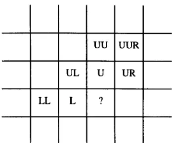
In image domain, prediction is often used. CALIC (Context-based Adaptive Lossless
Image Coding) is one of the successful candidates for predictive coding [2]. The
image pixels are coded in raster scan order (from left to right in a row, then down to
the next row). Current coding pixel is predicted according to a few neighbours, as
indicated in Figure 1.1. The prediction is adjusted according to the gradient in the
neighbourhood, to reflect the classified horizontal or vertical edge type - sharp,
normal, weak, or flat. The prediction error is coded using context -based arithmetic
coding. The context used for arithmetic coding is the texture information of selected
neighbours with respect to the predicted value, plus the quantised energy of previous
prediction error. For each context, the expectation of prediction error is fed back to
UU UUR
UL U UR
LL L ?
Figure 1.1 Neighbours used for prediction in CALIC ?
=
Pixel to be coded, U=
Up, R=
Right, L=
LeftHere we concentrate on transform coding. Figure 1.2 shows the framework of a
transform coding system. Image pixels are transformed to coefficients on subbands,
then the coefficients are quantised and entropy encoded. On the decoding side, the
reverse is done - the encoded bit-stream is entropy decoded and de-quantised
(dequantisation here means mapping of codes to values of coefficients), and the
resulting coefficients are inverse transformed to reconstruct the image.
Image pixels
Image pixels
~
....
..
Forward..
Quantisation
...
transform
...
Inverse ... De- ...
[image:26.480.156.330.49.194.2]transform .... quantisation ....
Figure 1.2 Transform coding system
Entropy
...
encode"
Entropy decode
Two transforms are widely used for transform coding: the discrete cosine transform
(DCT) and the wavelet transform.
The DCT is orthogonal, and is used to de-correlate the image data so as to reduce its
Chapter 1. Introduction 7
In JPEG, an image is divided into blocks of 8x8 pixels. Then two-dimensional (20)
OCT is applied to the image blocks. The coefficients in the transform domain are
quantised and entropy coded.
Recently the wavelet transform has shown its advantages in image coding. The
advantages include not only the high rate-distortion performance, but also the
scalability of coding rate and PSNR. Embedded zerotree wavelet coding (EZW) [4],
set partitioning in hierarchical trees (SPIHT) [5], and embedded block coding with
optimised truncation (EBCOT) [6] are three well-known representatives. They have
two key concepts in common, as described in the following two paragraphs.
The first is successive approximation quantisation of wavelet coefficients. The
wavelet coefficients are quantised using a gradually refined threshold other than a
fixed value. Usually the quantisation threshold is reduced by half in each round of
the coding. The coding is in fact a binary bit-plane coding. The wavelet coefficients
are coded bit-plane by bit-plane, from the most significant bit (MSB) to the least
significant bit (LSB).
Second, the three algorithms exploit in different ways the facts that neighbouring
pixels of an image are often continuous in value and that the edges of objects in an
image tend to cluster together. Neighbouring wavelet coefficients from a squared
region are grouped together in a set for coding in the EZW and SPIHT algorithms.
EBCOT uses context based models for arithmetic coding, where a wavelet
coefficient is entropy coded according to the conditional probability under the
condition of the latest known status of neighbouring wavelet coefficients.
EZW set up the foundations of the successful novel embedded wavelet image
coding - this is exclusive to SPIHT. EBCOT, the most recent one, is adopted as the
basic encoding engine in the new international standard JPEG 2000 [7].
1.2.2
Physical models
Video coding based on physical models has been successful, for example,
motion-compensated video coding in MPEG-l and MPEG-2 [8], and object-based video
coding in MPEG-4 [1]. They are based on the natural characteristics of the objects in
the video, and the physical formation of the video signal (e.g. the projection of
three-dimensional objects on a two-three-dimensional plane, and the effect of camera movement
such as pan, zoom in/out, rotation, tilt, etc.).
The similar concept can be used in image coding. The objects can be separated from
the background in the image. If the shape of the object is regular, and the colour of
the object is consistent, the object can be encoded separately, to get the most
compression.
Due to its complexity, image coding based on physical models has not been studied
very much.
1.3 Research objectives
This research is on the SPIHT algorithm. The objective was to investigate various
aspects of SPIHT image coding, such as the wavelet transform, organisation of
wavelet coefficients, quantisation, and entropy coding. This included exploring
statistical properties of wavelet coefficients of natural images, developing novel
algorithms for image compression, and applying them in image coding applications.
In chapter 2, the wavelet transform for image coding is discussed. Chapter 3 explores
the statistical properties of wavelet coefficients of natural images. Chapter 4
Chapter 1. Introduction 9
improve SPIHT, and chapter 7 is the numerical results of the improvements for lossy
image coding. In Chapter 8, the SPIHT algorithm and the new improvements are
applied to lossless image coding. Performance evaluation is done for various
reversible integer-to-integer wavelet transforms. Chapter 8 also gives some of the
attempts on image coding based on physical models - content-based SPIHT coding
for CT head image. Chapter 9 concludes the thesis.
This research started before EBCOT was published and JPEG 2000 was established.
Although EBCOT outperforms SPIHT in some aspects, SPIHT still has its exclusive
advantage. Besides, as shall be seen, some of the research results for SPIHT are
References
[1] T.Ebrahimi and C.Home, 'MPEG-4 Natural Video Coding - An Overview',
Signal Processing: Image Communication, Vol. 15, No.4-5, pp.365-85, Elsevier
Science, 1anuary 2000.
[2] X.Wu and N.Memon, 'Context-based, Adaptive, Lossless Image Codec', IEEE
Transactions on Communications, Vol.45, No.4, pp.437-44, April 1997.
[3] W.B.Pennebaker and 1.L.MitcheI1. 1PEG still image data compression standard.
Van Nostrand Reinhold, New York, 1993.
[4] 1.M.Shapiro, 'Embedded Image Coding Using Zerotrees of Wavelet
Coefficients', IEEE Transactions on Signal Processing, Vo1.41, No.12, pp.3445-62,
December 1993.
[5] ASaid and W.APearlman, 'A new, fast, and efficient image codec based on set
partitioning in hierarchical trees', IEEE Transactions on Circuits and Systems for
Video Technology, Vo1.6, No.3, pp.243-50, 1une 1996.
[6] D.Taubman, 'High performance scalable image compression with EBCOT',
IEEE Transactions on Image Processing, Vo1.9, No.7, pp.1158-70, July 2000.
[7] ASkodras, C.Christopoulos and T.Ebrahimi, 'The 1PEG2000 Still Image
Compression Standard', IEEE Signal Processing Magazine, Vol.I8, No.5, pp.36-58,
September 2001.
[S] 1.L.Mitchell, et al. MPEG video compression standard. Van Nostrand Reinhold,
Chapter 2
The Wavelet Transform
This chapter describes some of the properties of the discrete wavelet transform
(OWT) that are pertinent to image compression. The wavelet analysis and synthesis
are reviewed, along with multi-resolution transform, and from one-dimensional (10)
to two-dimensional (20) transform. The relationship of the filter banks and the
wavelet transform (WT) are explored, with emphasis on the biorthogonal case.
Image edge extension for WT are discussed.
2.1 Two-channel filter banks
To understand 20 wavelet analysis and synthesis for image coding, we start with
two-channel filter banks, as shown in Figure 2.1. Here we take a brief review, with
emphasis on perfect reconstruction (PR) which leads to biorthogonal filter banks.
More details can be found in [1] - [6].
r ___________ ~_~~ly~l~
________ .
....----,
.
:L
La(z)
{,2
~~r---~YP1~~~1~
_________ _
•
Ls(z)
x(n) x(n)
Ha(z)
HHs(z)
The analysis filter banks are inside the left dashed box of Figure 2.1, and the
synthesis filter banks are inside the right box. The signal x(n) is filtered by lowpass and highpass analysis filters - La(z) and Ha(z) , and then down-sampled
(decimated) by 2 (denoted by J..2 in Figure 2.1). The analysis filter banks decompose
x(n) and produces two subbands: the low (L) and high (H) subbands. The decomposed signals are
l(k) = Lla(2k - n)x(n)
• (2.1)
h(k)
=
L ha(2k - n)x(n) •To reconstruct x(n), The Land H signals are up-sampled (stretched) by 2 (denoted
by i2 in Figure 2.1), interpolated with zeros, and then filtered by lowpass and
highpass synthesis filters - Ls(z) and Hs(z). The results from the two channels are added up to the reconstructed signal:
x(m) = ~)ls(m-2k)l(k)+hs(m-2k)h(k)] k
Insert (2.1), we get
x(m)
=
Lx(n) ~:Cla(2k - n)ls(m -2k) + ha(2k - n)hs(m- 2k)] (2.2)n k
We use the z-transform to analyse the filter banks. For a sequence x(n),
X(z) = Lx(n)z-n . X(z) becomes [X(Zll2)
+
X(-il2)]12 if down-sampled by 2, andn
becomes X(l) if up-sampled by 2.
In Figure 2.1, the results of analysis are
L(z)
=
[La(zll2)X(i12)+
La(-il2)X(-ll2)]12H(z)
=
[Ha(i12)X(zll2)+
Ha(-zll2)X(-i12)JI2The synthesis result is
X(z) = Ls(z)L(Z2)
+
Hs(z)H(Z2 )Chapter 2. The Wavelet Transform
Insert (2.3), we get
x
(z) = [La(z)Ls(z)+
Ha(z)Hs(z)]X (z)1 2+
[La(-z)Ls(z)+
Ha(-z)Hs(z)]X(-z)/2To get PR, for any x(n), x(n)
=
x(n). For (2.4), this impliesLa(z)Ls(z)
+
Ha(z)Hs(z)=
2 La(-z)Ls(z)+
Ha(-z)Hs(z) = 013
(2.4)
(2.5)
(2.6)
(2.5) and (2.6) are necessary and sufficient conditions for PRo In the time domain, as
can be seen from (2.2), they are equivalent to
L[la(2k - n)ls(m - 2k)
+
ha(2k - n)hs(m - 2k)]=
Oem - n) (2.7) kIf we exchange La(z) with Ls(z) and Ha(z) with Hs(z), (2.5) - (2.6) or (2.7) still hold.
In other words, {La(z), Ha(z)} and {Ls(z), Hs(z)} are interchangeable.
2.2 Biorthogonal filter banks
We shall see in this section that PR filter banks are biorthogonal. Stephane Mallat
proved this in [1] through the Fourier transform. Here we present a detailed proof in
z-domain.
From (2.5) and (2.6), Ls(z) and Hs(z) can be expressed by La(z) and Ha(z):
Ls(z)
=
-2·Ha(-z)ID(z) (2.8)Hs(z)
=
2·La(-z)/D(z)(2.9)
Where D(z)
=
La(-z)Ha(z)-La(z)Ha(-z). It can be verified that D(-z)=
-D(z). From (2.8) and (2.9), we get, respectively,Ha(z)
=
Ls(-z)D(z)12 La(z)=
-Hs(-z)D(z)12 Insert (2.9) and (2.10) into (2.5), we getLa(z)Ls(z)
+
La(-z)Ls(-z)=
2(2.10)
(2.11)
Insert (2.8) and (2.11) into (2.5), we get
lIa(-z)lIs(-z) + lIa(z)lIs(z)
=
2 Rewrite (2.8) and (2.11):lIa(-z) = -Ls(z)D(z)12 lIs(-z)
=
-2La(z)ID(z)From (2.10) and (2.14), we have
Ls(z)lIa(z)
+
Ls(-z)lIa(-z)=
0From (2.9) and (2.15), we have
La(z)lIs(z)
+
La(-z)lIs(-z)=
0In time domain, (2.12) - (2.13) and (2.16) - (2.17) mean, respectively,
LLs(n)La(2k -n) = t5(k)
n
Lhs(n)ha(2k -n)
=
t5(k)n
Lfs(n)ha(2k - n)
=
0n
Lhs(n)fa(2k -n)
=
0n
Denote La (n)
=
far-nY, and ha(n) = ha(-n). (2.18) - (2.21) becomeLLs(n)la(n - 2k) = t5(k)
n
Lhs(n)ha(n - 2k)
=
t5(k) nLLs(n)ha(n - 2k)
=
0n
Lhs(n)La(n-2k) =0
Chapter 2. The Wavelet Transform 15
The relations (2.22) - (2.25) are known as biorthogonality, and La(z), Ls(z) , Ha(z) and Hs(z) are called biorthogonal filter banks. We see here that general PR filter banks are biorthogonal.
2.3 Perfect reconstruction FIR filter banks
As a special case of biorthogonal filter banks, PR FIR filter banks can have linear
phase, which is often desired in practice. As we shall see, PR FIR filter banks are
used throughout the thesis.
We explore the relations of filters for PR FIR filter banks. We follow similar steps as
in [2], but not the same, and we give more details.
If we use FIR (finite impulse response) filters, La(z), Ls(z), Ha(z) and Hs(z) can be written as a product of a polynomial in Z-I with an integer power of i l . Notice that
for every root of La(-z) (root for iI, same afterwards) there is an equal and opposite root of La(z), and the roots of Ha(-z) are also equal and opposite to the roots of
Ha(z). So La(-z) and Ha(-z) have no zeros in common otherwise the PR condition of (2.5) could not always hold. It follows from (2.6) that Ls(z)
=
0 whenever Ha(-z)=
0, and Hs(z)=
0 whenever La(-z)=
O. We can write Ls(z) in the formLs(z)
=
Ha(-z)p(z) (2.26)Where p(z) is also a product of a polynomial in
i
l with an integer power of Z-I.Substitute (2.26) into (2.6), we get
Hs(z)
=
-La(-z)p(z) (2.27)Similarly, Ls(z) and Hs(z) have no zeros in common because of (2.5). It follows from
(2.6) that La(-z)
=
0 whenever Hs(z)=
0, and Ha(-z)=
0 whenever Ls(z)=
O. ConsequentlylA2(-z)
=
-lIs(z)q(z) (2.29) Where q(z) is again a product of a polynomial in Z·I with an integer power of i l .Substitute (2.28) into (2.26), we get
p(z)q(z)
=
1 (2.30)Recall that p(z) and q(z) are both products of a polynomial in
i
J with an integer power of z·J. The only possible solution for (2.30) isp(z) = el
( ) ·I·k
q Z =e Z
(2.31)
(2.32)
Where e is a constant (e;t(J) and k is an integer. Substitute (2.32) into (2.28), we get lIa(z)=(-1 /e·1 z·kLs(-z)
Substitute (2.31) into (2.27), we get
IIs(z)
=
-cllA2(-z)Insert (2.33) and (2.34) into (2.5), we get
lA2(z)Ls(z) - (-l/lA2(-z)Ls(-z) = 2
For (2.35) to hold, k can only be odd, k=2K + 1. Then (2.33) - (2.35) become lIa(z)=-e·1 i 2K•1 Ls(-z)
IIs(z)
=
_CZ2K+JlA2(_z)lA2(z)Ls(z) + lA2(-z)Ls(-z) = 2 In time domain, (2.36) - (2.38) means
ha(n)=(-l t-c·1 ·ls(n-2K-1)
hs(n)=( -I t·e ·la(n+2K
+
1)Lis(n)ia(2k - n)
=
8(k) n(2.33)
(2.34)
(2.35)
(2.36)
(2.37)
(2.38)
(2.39)
(2.40)
(2.41)
Chapter 2. The Wavelet Transform 17
ha(n) = (-It ls(1- n) (2.42)
hs(n) = (-It la(l- n) (2.43)
Ils(n)la(n- 2k)
=
o(k) (2.44)n
The relation (2.42) to (2.44) are very important and well known for the PR FIR filter
banks.
2.4 Wavelet transform
Now we explain the relations between the filter banks and the WT. First we build the
WT from the filter banks, and then get the filter banks from the WT. For generality,
the biorthogonal case is used for analysis. As we shall see later, the orthogonal WT
is a special case of biorthogonal WT.
2.4.1
Scaling function
The dilation equations define the scaling functions ~t) and ip (t):
rp(t) = JiIla(n)rp(2t - n) (2.45)
n
ip(t) = ..J2Ils(n)ip(2t - n) (2.46)
n
qX.t) and ip (t) satisfy the biorthogonal relations:
(rp(t), ip(t - n») = o(n) (2.47)
Where (x(t), yet») is the inner product of x(t) and yet). (x(t), yet») =
1
x(t)y(t)dt .Denote rpj,dt)
=
ff2~it-k), and ip j,k(t)=
ff2 ip (it-k). For fixed j, f/1,k(t) spans Vj ,and ip j,lt) spans
V
J. It can be seen that VJc
VJ+l'V
J CV
j+l, andrpj,k (t) = Ila(n)rpj+\,2k+n (t) (2.48)
ipj,k(t) = I,ls(n)ipj+I,2k+n(t) (2.49)
n
2.4.2 Wavelet
The wavelet equations define the wavelet w(t) and
W
(t):wet) = J2I,ha(n)({J(2t - n) (2.50)
n
W(t) = J2I,hs(n)ip(2t -n) (2.51)
n
Denote wj,dtJ
=
ff2w(it-k), andW
j,k(t) =ff2
W
(it-k). For fixed j, wj,dt) spans Wj,and
W
j,k(t) spansW
j. It can be seen that Wj c Vj+hW
j CV
j+l, andWj,k (t) = I,ha(n)({Jj+I,2k+n (t) (2.52)
n
(2.53)
n
2.4.3 Wavelets from filter banks
Now suppose La(z), Ls(z) , Ha(z) and Hs(z) are PR filter banks. (2.7) is satisfied.
La (z), Ls(z) , Ha (z) and Hs(z) are biorthogonal, as related by (2.22) to (2.25). We build the biorthogonal WT. The key is to prove the biorthogonal relations of qJj,k(t),
iP
j,lt) , Wj,k(t) andW
j,dt):(Wj,m (t),
wj,n (t»)
= 8(m - n)(((Jj,m(t),
wj,n(t»)
= 0Although a proof can be found in literature, we present our own proof here.
By definition, we have
(2.54)
(2.55)
(2.56)
Chapter 2. The Wavelet Transform 19
(({Jj,m(t),iPj,n(t)) =
J
({Jj,m(t)'Pj,n(t)dt t=
J
2jl2 ({J(2j t - m)· 2j/2 'P(2j t - n)dt tLet T = 2 j t - m ,
(({Jj,m (t), 'Pj.n (t)) =
J
({J(T)'P(T + m - n)dTr
Applying (2.47), we obtain (2.54).
Similarly, by definition and applying (2.52) and (2.53), we have
(Wj,m(t), wj.n(t)) = f Wj.m (t)wj,n (t)dt t
= fLha(l)({Jj+l,2m+l (t)· Lhs(k)'Pj+l.2n+k (t)dt
t I k
=
LLha(l)hs(k)J
({Jj+l.2m+l (t)'Pj+l,2n+k (t)dt k i tApplying (2.54):
(W
j,m (t), W j.n (t») = L L ha(l)hs(k )O(2m+
1-2n - k)k I
= Lhs(k)ha(k - 2m
+
2n) kApplying (2.23), we obtain (2.55).
By definition and applying (2.48) and (2.53), we have
(({Jj,m (t), Wj,n(t)) =
J
({Jj,m (t)w j .n (t)dt t= f L 1a(l)({Jj+l.2m+1 (t)· Lhs(k)'Pj+l,2n+k (t)dt
t I k
= LLhs(k)la(l) f ({Jj+l,2m+1 (t)iPj+1.2n+k (t)dt
k I t
Applying (2.54):
(({Jj.m (t), wj •n (t)) = LLhs(k)la(l)O(2m
+
1-2n - k)k I
=
Lhs(k)la(k-2m+2n)k
By definition and applying (2.49) and (2.52), we have
(ip j.m (t), W j,n (t)) = f ip j,m (t)w j,n (t)dt
t
=
fI/s(k)CPj+l,2m+k (t). Lha(l)qJj+l,2n+l (t)dtt k I
= LLls(k)ha(l) f qJj+l,2n+l(t)CPj+l,2m+k (t)dt
k i t
Applying (2.54):
(CPj,m (t), Wj,n (t»)
=
LLls(k)ha(l)8(2n+
1-2m - k)k I
=
Lls(k)ha(k-2n+2m)k
Applying (2.24), we obtain (2.57). The proof is completed.
(2.56) says
W
j .1 Vj, and (2.57) says Wj.lV
j. Now we check the relationship ofV
j+l,V
j andW
j. Any J(t) EV
j+l can be expressed asJ(t)
=
La j+l,kCPj+l,k (t) (2.58)k
It follows from (2.58) and (2.54) that
I n
= Laj+1,nJ ({Jj+l,k(t)CPj+1.n(t)dt
n I
= laj+I,n8(k -n)
n
= a j+I,k
That is
a j+I,k = (/ (t), qJ j+1.k
(t»)
(2.59)Define
(2.60)
(2.61)
Chapter 2. The Wavelet Transform 21
a j,k =
f
[ I a j+l,ntPj+l,n (t)]{Lla(m)~j+I,2k+m
(t)]dtt n m
=
I I
a j+l,n la(m)f
~
j+I,2k+m (t)tP j+l,n (t)dtm n t
Applying (2.54):
m n
= Ila(n - 2k)a j+l,n
n
That is
aj,k = Ila(2k -n)aj+l,n (2.62)
n
Similarly, insert (2.58) and (2.52) into (2.61), and apply (2.54), we obtain:
bj,k
=
Iha(2k - n)a j+l,n (2.63)n
Now with (2.49), (2.53), (2.62) and (2.63), we have
Iaj,ktPj,k(t)
+
Ibj,kWj,k(t)k k
= I[Ila(2k - n)a j+l,n]' [Ils(m)tPj+I,2k+m (t)]
k n m
+
I[Iha(2k - n)a j+l,n]' [Ihs(m)tPj+I,2k+m (t)]k n m
Let 2k+m
=
i,Ia
j,ktPj,k (t)+
Ibj,k Wj,k (t)k k
= I[Ila(2k - n)a j+l,n]' [IZs(i - 2k)tP j+I,;(t)]
k n i
+
I[Iha(2k - n)a j+l,nl' [Ihs(i - 2k)tPj+l,i (t)]k n i
=
IIa
j+l,ntPj+l,i I[la(2k - n)ls(i - 2k)+
ha(2k - n)hs(i - 2k)]n i k
Applying (2.7),
Ia
j,ktPj,k (t)+
Ibj,k Wj,k (t)k k
= I I a j+l,ntPj+l,it5'(n-i)
n i
=
I
a j+l,n tP j+l,nApplying (2.58), we obtain
~>j,kq;j,k(t)+ Lbj,kWj,k(t) = f(t)
k k
Or rewrite as
f(t)
=
La j,kq;j,k (t)+
Lbj,k Wj,k (t) (2.64)k k
(2.64) means that
V
j EeW
j ~V
j+l. BecauseV
j CV
j+l andW
j CV
j+l, we haveSimilarly, we have Vj+l = Vj Ee Wj.
According to the relations, we can decompose a function in a high level by the
scaling function of the low level and the wavelet. The wavelet part is the details that
represent the complement between the high resolution and the low resolution.
Repeating the relations for various j, we have
This suggests the multi-resolution decomposition, which is to be discussed in the
next section.
ACohen, Ingrid Daubechies, and J.-C. Feauveau proved in [2] that in the FIR case,
wj,it) constitute a frame in L2(R), and Wj,k(t) and W j,k(t) constitute dual Riesz bases.
2.4.4 Filter banks from wavelets
Now inversely, we get the filter banks from the WT. We can easily get the fast WT,
(2.62) and (2.63), from biorthogonal wavelets [1 ][5]. (2.62) means that filtered by
La(z) and sub-sampled by 2, we get aj,k from aj+l,k. while (2.63) means that filtered
Chapter 2. The Wavelet Transform 23
On the other hand, we can get (2.22) to (2.25) from (2.54) to (2.57) [3]. That is,
La(z), Ls(z), Ha(z) and Hs(z) are biorthogonal. As can be verified, Ls(z) and Hs(z)
constitute the two-channel synthesis filter banks with PR.
2.4.5 Summary and example
If we impose qi,t) = ip (t) or Ls(z) = La (z), the biorthogonal WT defined by (2.45) to (2.53) becomes orthogonal WT, and the biorthogonal filter banks become
orthogonal filter banks.
Now with the relations between the filter banks and the WT, we can choose filters
from a wide range of wavelet families for subband decomposition.
As an example, Table 2.1 gives the filter coefficients of the biorthogonal 917 WT [2],
which is very popular for image coding. It is symmetric.
Table 2.1 Filter coefficients of biorthogonal 9/7 wavelet transform
n la(n) 1.J2 ls(n) 1.J2
0 0.602949018236 0.557543526229
±1 0.266864118443 0.295635881557
±2 -0.078223266529 -0.028771763114
±3 -0.016864118443 -0.045635881557
±4 0.026748757411 0
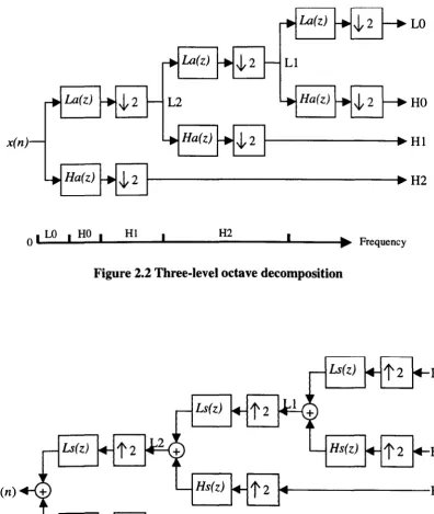
2.5 Multi-resolution decomposition
A signal can be decomposed into multi-levels or subbands using two-channel filter
input signal is decomposed into two subbands, and the decomposition is iterated on
the low subband output signal. This results in octave decomposition in the frequency
domain, as shown on the scale at the bottom of Figure 2.2.
x(n)
~2
LO
HO
1---...
HI~---~H2
o
I LO I HO I HI H2 I • Frequency [image:44.481.46.442.157.626.2]x(n)
Figure 2.2 Three-level octave decomposition
Ls(z) LO
Ls(z)
t
2Hs(z)
HO
t2 I + - - - H I
~---H2
Chapter 2. The Wavelet Transform 25
The octave decomposition is identical to multi-scale WT, as supported by the
wavelet theory discussed in section 2.4. From the wavelet point of view, Figure 2.2
is three-scale WT. Take x(n) as a3,n in (2.59), which is an analysis coefficient of WT
on
V
3, then L2, LI, and LO are coefficients onV
2,V
1, andV
0 respectively, and H2, HI, and HO are coefficients onW
2,WI,
andW
0 respectively.Figure 2.3 does the opposite of Figure 2.2: three-level octave reconstruction. It is just
the reverse of Figure 2.2, replacing the analysis filters with the synthesis filters and
down-sampling with up-sampling.
The octave decomposition is widely used for multi-resolution decomposition.
2.6 Two-dimensional wavelet transform
The previous sections discussed the 1 D WT. For 2D images, we need the 2D WT.
We can extend the ID WT to 2D WT simply by applying the ID WT to the two
spatial dimensions separately. In this case, the corresponding transfer function
B(z]' zz), where z/ and zz relate to the two spatial dimensions, is separable, B(zl, zz)
=
B!Czl)Bz(zz). Non-separable B(z/, zz) is much more complex mathematically. As a polynomial of two variables, factorisation is not possible ingeneral. It is beyond our discussion.
Figure 2.4 shows the separable 2D wavelet analysis. First, 1 D horizontal filter banks
are used for each rows of the 2D image pixels, x(m,n), resulting in the horizontal low (L) and high (H) subband. Then, 1 D vertical filter banks are applied to each columns
of Land H, resulting in four subbands: LL, LH, HL, and HH, where the first letter of
the two- letter acronym denotes the horizontal L or H subband and the second
denotes the vertical L or H subband. The same filter banks are used for horizontal
Horizontal filter
____
iAI~_l!.g !~_~~2 ___ _
x(m,n)
Vertical filter
__J~~~l}g_~<!!l!I]!I}~L_
Figure 2.4 2D separable wavelet analysis
Horizontal filter Vertical filter
LL
LH
HL
HH
r---{~}~p~!~~~l---,
r - - -~~~~I!~LC:~~~~I!~_
---,
i(m,n)
,
,
,
,
,
,
,
:L
._---,
Figure 2.5 2D separable wavelet synthesis
LL
LH
HL
Chapter 2. The Wavelet Transform 27
Figure 2.5 shows the 2D separable wavelet synthesis. It is just the reverse of the 2D
separable wavelet analysis, with synthesis filters for analysis filters and up-sampling
for down-sampling.
For 2D multi-resolution decomposition, the 2D wavelet analysis in Figure 2.4 is repeated on LL. As the result, 3-scale 2D WT produces 10 subbands, as shown in
Figure 2.6. We call the resulting data in the transform domain wavelet coefficients
(WC).
LLO HLO HLI HL2
LHO HHO
LHI HHI
LH2 HH2
Figure 2.6 Subbands of 3-scale wavelet transform
2.7 Edge extension
When an input signal of length M is convolved with a FIR filter of length N, the
The solution is to take the finite length input as part of a periodic signal. We know that the output is periodic, and the period is the same as the input. We can keep only a period of the output without losing any information. Now we discuss the formation of the periodic signal.
The direct method is to repeat the input periodically, as shown in Figure 2.7. In practice, the signal is normally longer than the FIR filters, and we just need to repeat M-l samples of the input in order to calculate a whole period of the output, as indicated in Figure 2.7. So, it is in fact edge extension. We call this method periodic extension.
Input Period
; :
~ Samples to calculate a period of output~
: : :
.
:. .
: :i
Filter length.i
Filter lengthi
:II1II .: :II1II ~:
ffil..;:: ..
illTI
ffil.:;: ..
illTI
Figure 2.7 Periodic extensionChapter 2. The Wavelet Transform 29
length (M = 2m
+
J), except the trivial Haar filters [1]. In practice, we just need the m samples added at both ends of the input in order to calculate all the output samplesthat are not redundant. As in periodic extension, we call this method symmetric edge
extension.
Period
J
Input
2
Figure 2.8 Symmetric extension
Notice that at the edge, the added samples in symmetric extension are from the
neighbours, and those in periodic extension are from the other end of the input. In
image coding, neighbouring image pixels tend to be similar (because they are
probably from the same area of the same object), while the pixels at different ends of
rows or columns are relatively far away and thus less correlated. So, at the edge in
transform domain, the output signal in the symmetric extension case is probably
smoother than that in the periodic extension case, while the later is likely to have
jitters. For better coding performance, we use symmetric extension except otherwise
stated.
Similar edge extensions were used for arbitrarily shaped visual object coding in [7],
and more edge extensions were discussed there. But to our knowledge, if we use
linear phase FIR filter banks, the symmetric edge extension presented here is the best
for image compression, and can retain PR no matter the input is of odd or even
The periodic extension and the symmetric periodic extension were also discussed in
[8]. But for the symmetric periodic extension presented in [8], the first and the last
input samples appear in the extended signal, without overlapping of these samples
for flipping and periodic repeat, as shown in Figure 2.9. If the input is of odd length,
it is not possible to get PR without expanding the signal length in WT, as explained
at the end of section 2.8.
1:1
I
2I
Period
1
Input
IN-q
:1
N IN-II
I
2 2Figure 2.9 Symmetric extension without overlapping
If we use IIR filters, it is difficult to find an arrangement without expanding the
signal length under the condition of PRo
2.8 Arrangements of wavelet coefficients
As discussed previously, the WT will keep the size of 2D signals. For a M
x
Nimage, the corresponding WCs are also of size M
x
N. For a k-scale WT, it is easy tokeep the signal size if M and N are integer mUltiples of 2k. But for images of
arbitrary size, the WT should be done carefully, especially the down-sampling and
up-sampling. Here we present a scheme, as shown in Figure 2.10 and Figure 2.11.
Input signal samples are numbered starting from 1. To use symmetric edge
extension, the filters are symmetric or anti-symmetric, and of odd length (2m+ 1 ).
2m+ 1 neighbouring input samples are multiplied with the 2m+ 1 filter coefficients in
Chapter 2. The Wavelet Transform 31
the 2m+ 1 input samples. After low-pass analysis filtering using La( z), we keep the
odd numbered samples by down-sampling. After high-pass analysis filtering using
Ha(z) , we keep the even numbered samples by down-sampling. The down-sampled outputs are also symmetric. The samples outside the boundary of the input are
redundant. They are rejected, keeping the output the same size as the input. On the synthesis side, the Hand L signals are up-sampled by inserting a zero between every sample, and then extending symmetrically at the edge to recover the symmetric
periodic signal before synthesis filtering.
In Figure 2.10, the total number of input samples is odd (2n+ 1). The high subband
output signal (H) is one sample shorter than the low subband (L). The edge extension
of L signal after up-sampling, for synthesis, is the same as that of the input for analysis. For H signal, an extra zero should be inserted at both ends before applying
the same edge extension as that for the input.
Edge .... Input (odd length) Edge extension ~ ... ... ... extension
· .. 1 3
I
2 1 2I
3I
4I
I
2n-1 1 2n 12n+1 2n 1 2n-1 I .. ·Edge
~I"l
L (odd numbered)~I"
Edgeextension extension
.. ·1 3
I
3 12n-1 1 12n+! 12n-]I
.. ·
Edge
2
~I"
H (even numbered)
t
Edgeextension extension
.. ·1 1 2 1 4 1 2n . 2n
I I
.. ·
Figure 2.10 Down/up-sampling and edge extension in case of odd length input