Device free sensing and deep learning : analyzing human behavior through CSI using neural networks

(1)

(2)

(3)

Abstract

Monitoring human beings is becoming a more pressing matter in this society. It is common these days for people to wear wearable sensors in the form of smartwatches or activity trackers in order to sustain a healthy lifestyle, increase activity or improve sport performances. The desire to monitor ourselves becomes apparent by how fast different technologies are being adapted into monitoring systems.

Device-free sensing is one of these new monitoring systems. This is a method that allows the monitoring and localization of humans through measuring the characteristics of these wireless signals. A method to do so is by looking at the way these signals propagate through the channel state information (CSI). Deep learning is an upcoming field within machine learning used to classify human activities. It attempts to replicates the way humans perceive information. Of all the techniques within deep learning, convolutional networks have proven to be capable of dealing with signal processing, yet it has not been widely adapted in human activity recognition through CSI.

This research presented in this thesis looks into how convolutional networks perform against current state-of-the-art systems through analyzing both static and dynamic activities. The experiments performed in this research were conducted with multiple participants over three days to investigate about the scalability. The findings indicate that for dynamic activities, convolutional networks achieve higher accuracies than static postures (98% and 60%). Scalability between participants and days falls short, but findings imply that this is due to a lack of data.

Keywords

(4)

(5)

Preface and acknowledgements

This research is part of the ’Create Health’ project at the Pervasive Systems group, located at the University of Twente, Enschede, and connects to research done by Prachi Bagave for her Master thesis Unobtrusive sensing using Wi-Fi signals. Introductory work started in January 2018 in the form of Research Topics (a 10 EC literature research course before the graduation project), after I was contacted by Nirvana Meratnia in December 2017. I was done with Research Topics at the end of April 2018, but I did not actually started to work on the project until June 2018, as I was awaiting a grade for another course.

This project has been an interesting learning experience for me and has taught me many things. At times, this project was terrorized by delays: at first it was waiting on hardware for two months, after which it became waiting for my com-puter and laptop to be done rendering images and training neural networks. I have learned a great deal about planning and organizing a large scale research and I have learned a lot about analyzing and gathering data. I will never forget to collect ground truth data in future experiments and I will not sit idle while waiting for results when I can do other things. However, the most important thing this project taught me is that I enjoy research and it was a great boost in for my PhD. I would like to offer my deepest gratitude to dr. Nirvana Meratnia for offering me a position in this project and by supervising me throughout the entirety of Research Topics and this final graduation project. She has offered me lots of helpful advice and always managed to motivate me to take the extra step. When I was stuck on the project, she would offer me insight and other opportunities to continue the project. It was thanks to her motivation I managed to finish my thesis in time.

For the hardware aspects of this project, I want to express my gratitude towards dr. ir. D.V. Le Viet Duc and ir. D.T.N. Nguyen for supplying me with the

(6)

appropriate hardware (the router and other attritbutes), as well as helping to combine all the hardware in a small node. Without their help, I would not have been able to create the nodes currently in use.

I would like to deeply thank Prachi Bagave for supplying me with her data and helping me develop a better understanding of the Linux CSI Tool and CSI in general. Without her data and help, I would not have been able to get as far with my research as I did.

I would also like to thank the rest of the Pervasive Systems group for the conversations and insights I gathered during the time of my graduation project and I hope to continue these conversations during my PhD at the Pervasive Systems group.

I also want to thank prof. dr. P.J.M. Havinga and ir. E. Molenkamp for freeing up the time to read my thesis and being part of my final presentation.

(7)

List of Figures

2.1 Example showing a radio wave in wireless communications . . . 12

2.2 Difference between low and high frequencies . . . 12

2.3 Figure showing difference in i) amplitude shift keying (ASK), ii) frequency shift keying (FSK), and iii) phase shift keying (PSK) . . 13

2.4 Examples of CSI packets collected during experiments. . . 19

2.5 H matrix inMATLAB. . . 20

2.6 SNR plotted across the subcarriers. Two sets are plotted as there are two transmitting antennas . . . 21

2.7 Amplitude of the signal plotted over the duration of the frames for subcarrier 1 . . . 21

2.8 Showing a wider model, thus with more ReLU at one place . . . 22

2.9 Showing a deeper model, thus with more (hidden) layers . . . 23

2.10 Showing the principle of a neural network . . . 28

4.1 Examples of Raspberry Pi . . . 44

4.2 Hummingboard i2eX Pro . . . 45

4.3 Gigabyte Brix IoT . . . 47

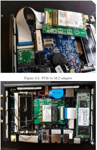
4.4 Inside of the Gigabyte Brix IoT. Note: while the antennas are dis-connected, this was merely to make the picture clearer: during all experiments, all antennas were connected. . . 48

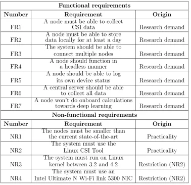
4.5 PCIe to M.2 adapter . . . 50

4.6 Final version of the modified Gigabyte Brix IoT . . . 50

5.1 Basic shapes drawn by hand . . . 58

5.2 Static postures performed during the research . . . 59

5.3 Different interpretations of CSI signals for the same activity and trial 63

[image:11.595.91.485.248.696.2]

(12)

third is the sliding window and the fourth (bottom) is the actual detection . . . 69

5.5 Visualization of the convolutional neural network used . . . 71

5.6 Different types of images rendered for this research . . . 72

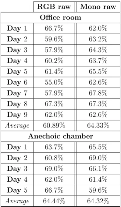
5.7 Figure showing the average accuracies per day in the office room

and anechoic chamber setup . . . 75

6.1 Basic shapes drawn by hand . . . 81

6.2 Difference between existing data set (left) and this research (right), also showing the overlap (middle). . . 82

6.3 Experimental setup in the studio . . . 84

6.4 Figure showing the accuracies per participants per day. Note that

the first day also offers information regarding slope and variance data 89

6.5 Figure showing the accuracies of each day overall and combinations

between days (training and testing) . . . 91

6.6 Figure showing the accuracies for combinations of training and clas-sifying with different numbers of participants per day . . . 92

6.7 Accuracies for individual days per participant and overall for same participants over multiple days. . . 93

6.8 Accuracies for training with one day and testing with another day . 94

6.9 Accuracies for training with two days and testing with another day 95

6.10 Slope analysis in monochrome for three activities . . . 96

(13)

List of Tables

4.1 Short overview of the (non-)functional requirements . . . 42

4.2 Overview of the hardware and their specifications . . . 43

4.3 Hardware specifications Gigabyte Brix IoT . . . 51

5.1 Overview of the activities, their summary, size of their data set and amount of CSI frames collected . . . 58

5.2 Table showing the classification rates for the existing data set, re-gardless of days (from [?]) . . . 73

5.3 Table showing the classification accuracies for individual days, as well as training with one day and classify with the other . . . 74

5.4 Table showing the accuracies per day and the average over all days

for static activities . . . 80

5.5 Table showing the accuracies between days for the static postures . 80

6.1 Table showing the times at which the experiments were conducted

for a given participant. Note that participant 1 and 2 are different for Day 1-3 and Day 6-8. . . 102

6.2 Table showing the classification rates when classifying for a single

participant (randomly ordered) for the first day . . . 103

6.3 Table showing the classification rates when training with two

par-ticipants and testing with the other for the first day . . . 103

6.4 Table showing the classification rates when training with one

par-ticipant and testing with the other two for the first day . . . 103

6.5 Table showing the classification rates when classifying for a single participant (randomly ordered) for the second day . . . 104

[image:13.595.94.493.253.708.2]

(14)

6.6 Table showing the classification rates when training with two par-ticipants and testing with the other for the second day . . . 104

6.7 Table showing the classification rates when training with one

par-ticipant and testing with the other two for the second day . . . 104

6.8 Table showing the classification rates when classifying for a single participant (randomly ordered) for the third day . . . 105

6.9 Table showing the classification rates when training with two

par-ticipants and testing with the other for the third day . . . 105

6.10 Table showing the classification rates when training with one par-ticipant and testing with the other two for the third day . . . 105

6.11 Table showing the classification rates when classifying for full days . 106

6.12 Table showing the classification rates when training with two days and testing with the other . . . 106

6.13 Table showing the individual classifications per participant per par-ticipant for strict data . . . 106

6.14 Table showing the average accuracies per day (overall) for strict data107

6.15 Table showing the average accuracies training for training and test-ing between different days (Day 6 and Day 7) . . . 107

6.16 Table showing the average accuracies training for training and test-ing between different days (Day 6, Day 7 and Day 8) . . . 108

[image:14.595.93.491.97.467.2]

(15)

(16)

Introduction

In our current society, the desire to monitor the world around is increasing. As technologies are advancing, it becomes easier to monitor and make life easier and more secure. Techniques are being used to make homes and cities smarter, prevent illegal poaching and thus help animal species threatened with extinction, structural health monitoring to aid in preventive maintenance, and monitor humans in their behaviour and health. Especially within monitoring humans, there are a lot of different fields. These include, but are not limited to, the monitoring of physical conditions to improve sport performance or to aid in recovery, monitor activities to aid in a smart home situation, or monitor medical symptoms to prevent and predict how diseases are progressing to call experts in case of an emergency. Currently, the most accessible and defined tool to monitor the aforementioned situations are wireless sensor networks.

Wireless sensor networks (WSN) have proven to be an important tool in con-tinously monitoring situations or detecting events and are often considered to be unobtrusive[1][2][3]. However, wireless sensor networks are not truly unobtrusive: they often require physical sensors worn on the structures or body parts. Wire-less sensor networks consist of a network of small, potentially different sensors, measuring the same or different aspects of the environment, but combining the information and data to come to conclusions. This means that situations are often measured directly: sensors can be put directly on the subject (building, human, animal) in question and thus the actions and events affect the sensor directly.

(17)

in-DEVICE-FREE SENSING & DEEP LEARNING

directly. Therefore, when it comes to truly unobtrusive sensing, the focus has more and more shifted to device-free sensing [4][5][6][7][8][9][10][11][12]. Device-free sensing uses the ”traffic” in the transmission environment generated by the actions or events caused by subjects and are thus often measuring the effects and impact of said actions and events, thus measuring the actions and events them-selves indirectly. While device-free sensing still uses nodes (laptops or routers) to measure the signals, they are often not part of the action (unlike wireless sensor networks) and are therefore considered to be truly unobtrusive.

In telecommunication, device-free sensing is often done through measuring the wireless medium, thus the radio waves that are traveling through the air. There are several techniques to do so, such as measuring the packet receiving rate (PRR) [5], received signal strength indicator (RSSI) [8] or the channel state information (CSI). Lately, it is believed that CSI is the best characteristic to look into, as it captures the entire propagation from transmitter to receiver [6][13][14][15][10][11][16][17][18][19]. None of these solutions measure the wireless medium directly, that is, listening to the frequencies and notify which frequencies are used. Instead of measuring the wireless medium directly, these solutions require one to send traffic through the medium and measure how this traffic is affected by the impact of the actions one wants to measure.

To understand the previous better, one can imagine two people separated by an ocean: they cannot directly see each other, making the only way to communicate with one another to create waves that eventually reach the other person. Even when sending the same message, the receiver will a difference in the waves each time: they could be taller, they could come in at a different angle, or the delay could be slightly larger. This is all caused by impacts on the water, which could be environmental (e.g. the wind), or actions by people (e.g. ships on the water, people on the shore fishing). Each of these activities has a specific signature on the water, and thus by analysing the waves received (by sending a known message), one could classify these activities. The same technique can be used for radio waves, albeit different characteristics due to the frequency spectrum being slightly more complex.

This technique of device-free sensing can be used in human activity recognition: detecting, classifying and monitoring humans has proven to be a demanding re-search field when it comes to device-free sensing [8][6]. Research currently focusses

(18)

on indoor localization through CSI analysis [14][20] and human activity itself [8][6]. An especially interesting field in this is the support for elderly or handicapped: cre-ating such systems allow automatic fall or aid detection, while increasing privacy, as current systems require either wearable sensors [21][22][23][24][25][26] or video cameras [27][28][29][30]. When it comes to health care (whether it is for the el-derly, handicapped or the average person), an important incentive to invest in device-free sensing is the ease of use: the wireless signals are already there, so one only requires a node (or several nodes) to measure the disturbances and warn in case of an emergency. This is much more convenient than wearable sensors, as one cannot expect the elderly or handicapped to always wear body sensors, nor can they be expected to always carry their phones or smartwatches. A device-free system also offers much more privacy than video cameras, in the sense that when people feel watched, they act differently and feel more uncomfortable (Hawthorne effect).

The most famous way to recognize human activity is machine learning. Ma-chine learning is the field in artificial intelligence that uses mathematical tech-niques (from structured data) to give computers the power to learn from data, without humans interfering with such a system. While such systems have proven to be accurate in human activity recognition (both for wearable sensor systems [31][32][23][24][26] as for device-free solutions [33][8][5][16][17]), these systems of-ten need to be trained by having structured data and by having the features picked by humans.

(19)

DEVICE-FREE SENSING & DEEP LEARNING 1.1. PROBLEM STATEMENT In deep learning, a distinction can be made into two main fields: convolutional networks (CNN) [3][34][20][35][19] and recurrent neural networks (RNN) [2][13][11]. The former focusses on recognizing and classifying of objects in images and the latter for recognizing and classifying recurring events (such as texts). Convolu-tional neural networks have been proven to work fine with CSI, as CSI can be classified as unstructured data and by analysing the graphs it will determine its own features.

1.1 Problem statement

Even though a lot of research goes into the analysis of CSI through convolutional networks, there are a few shortcomings. The first of which is the size of the nodes: these are usually full-sized computers or laptops, which are not at all convenient to place around rooms in inobtrusive manner. If the technology is to be used in practice, for example in health care to support the elderly, the nodes must be smaller in order to be more easily placed around a room.

Secondly, while plenty of research goes into human activity recognition and detection, research falls short when it comes to looking at the scalability of their solutions: it is often only one or two subjects for which the data is collected. If a system is to work properly in a real-life setting, the system must work for humans with a lot of different characteristics: height, weight, gender and style.

Lastly, different research often uses the same characteristic of CSI: the ampli-tude and phase. It is possible that other characteristics of the CSI provide more information. One of these characteristics is the slope analysis of the CSI data: slopes give a lot of information regarding how fast a change occurred, rather than how impactful the change was (amplitude).

1.1.1 Research aim and questions

The main aim of this research is to give insight in how convolutional networks can be used to classify human behaviour through measuring disturbances in the channel state information. More specifically, the focus will be on giving give insight in whether or not it is feasible to use convolutional network to classify behaviour and activities between different people.

(20)

Furthermore, this research aims to create CSI collecting nodes smaller than the current state of the art, in order to make the nodes more mobile and therefore more functional. Smaller nodes are easier to put in rooms and to leave unattended, rather than having entire laptops or computer collecting the CSI.

The main research question for this research is: What is the influence of multi-ple peomulti-ple and days on CSI when classifying human activity through deep learning. This research emphasizes convolutional network, as this is a promising deep learn-ing technique and this is thus compared to the current state-of-the-art. In order to answer this question, multiple research questions will be answered:

RQ1 What is the correlation between feature extraction and the accuracy of CNNs when classifying human activities using a single node?

RQ2 What is the correlation between combining data of participants for train-ing/classification and the accuracy of the system?

RQ3 What is the correlation between combining data of participants for train-ing/classification and the accuracy of the system?

It should be noted that part of this research is dedicated to creating nodes smaller than the current state-of-the-art. This has to do with the current nodes not being small enough to unobtrusively place nodes around a room. As future research involves multiple nodes in a single room, it is important to create a smaller node.

1.2 Research overview

The research started by laying out the current state-of-the-art methodology and hardware through an extensive literature research. The start of the literature research was made in another paper, done for the course Research Topics.

(21)

DEVICE-FREE SENSING & DEEP LEARNING 1.2. RESEARCH OVERVIEW these worked properly: the Raspberry Pi 3 failed because of hardware limitations, whereas the Hummingboard Edge i2eX failed due to a combination of hardware and software limitations. In the end, a small, barebone computer (Gigabyte Brix IoT) was modified in order to fit the components and function properly. To finish of the first part of the research, software was written that allowed i) adaptable CSI collection, ii) synchronizing the data to a central server, and iii) collect device status data.

Secondly, existing data was used to familiarize with the CSI data, as well as verify the functionalities of convolutional networks in these situations. The data used consisted of multiple activities and locations: i) sit and stand, ii) basic shapes (five basic hand movements), iii) static postures (five postures for which the CSI was measured), iv) multiple day data and v) standard activities (doing nothing, clapping, walking, jogging and jumping). First, it will be explained what data and how it was fed into the convolutional neural network. To finish the second part of the research, the network is trained for all of the aforementioned activities and the performance is compared to the results of the research from which the existing data originates. For static postures, the current implementation of the neural network scores lower than the previous research. However, for the dynamic activities, the convolutional network outperformed previous research in multiple cases.

Lastly, the experiments for this research were conducted. The activities were performed in an actual living room environment over the course of three days. Participants were encouraged to perform activities differently, in order to view how this would impact accuracies both per day and over different days. Another group of participants were asked to perform activities consistently over multiple days. Also, interference was added by always being engaged in conversation with the participants, as well as performing small tasks next to them. Accuracies were high for individual participants and even considerably high between participants on a given day. Accuracies dropped when classifying for a group of participants and trying to classify the others. Accuracies also dropped for classification for a single participant over multiple days, but not as low as for different participants. However, it seems likely that more data would greatly increase the accuracy of the system.

(22)

1.3 Thesis overview

After the introduction, background information will be given on both wireless sig-nals (section2.1) and deep learning (section 2.2). In general, it is recommended to read through these chapters as they can be a refresher to knowledge and further-more, to lead immediately into the knowledge required to understand this research. Having a lack of knowledge in either of these fields, it is strongly recommended to read these chapters. In wireless signals, the basics regarding frequencies, modula-tion and influences will be discussed. This is necessary to understand the analysis of networks through RSSI, SNR and CSI, all of which are discussed in the back-grond afterwards. Finally, a quick look into CSI analysis through MATLABis given. For deep learning, the section first explains the basics of a neural network: the softmax function, cross entropy and (stochastic) gradient descent, as well as the different layers, propagations and regularizations. After these basic concepts, the two main neural networks are explained: convolutional and recurrent neural networks, respectively. Also, not just the basic principles of these neural nets are explained, also the main differences and their strengths are explained.

After the background, the state-of-the-art is listed and explained in section 3.1. A distinction is made between two main subjects: unobtrusive human ac-tivity classification through device-free sensing and analysing networks and their disturbances, respectively. After listing and explaining the state-of-the-art, the state-of-the-art is discussed and the main strengths and shortcomings are pointed out.

Next, the hardware creation is discussed. First, the requirements for the nodes are listed in section 4.1. These requirements are split in the functional and non-functional requirements. After the requirements are presented, a look is taken into possible solutions and ideas to create such a wireless node and the shortcomings of the attempted solutions. The chapter is concluded by given the specifications to the final hardware, as well as giving the written software to create an understanding on how the node (and a network of these nodes) work.

(23)

DEVICE-FREE SENSING & DEEP LEARNING 1.3. THESIS OVERVIEW of the mentioned methodology are mentioned next, together with the alternative approach provided by this research and the results of the alternative approach.

In chapter 5, the experiments that belong to this research are conducted and explained. First, the new list of activities is listed: walking, running, jumping, falling, clapping and sitting. It is then explained how this data is gathered and analysed in the methodology, after which the experimental setup is explained and finally the results of the conducted research.

The final two chapters are the conclusion and future work, respectively.

(24)

Background

2.1 Wireless signals

Wireless signals are considered to be radio signals carried through the air.

2.1.1 Frequencies and channels

First, to understand the definition of a channel, one must understand frequencies. The technical definition of a frequency is the number of recurring events per second; thus, formally described a frequency f in Hz (Hertz) can be described as

f = 1 T

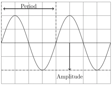
whereT is the period of a single event in these repetitions in seconds ([36], p. 29). Frequencies, combined with amplitude and their period, can be represented as a radio wave in a graph, as shown in figure2.1. Combining this with a phase, it can be expressed in the following formula (known as a sinusoid) ([36], p. 29):

s(t) = Asin(2πf t+φ)

To give an example within the field of wireless communications, suppose a low frequency signal A and high frequencyB, of which the period is 4 times smaller. The difference in their period can be seen in figure 2.2.

(25)

DEVICE-FREE SENSING & DEEP LEARNING 2.1. WIRELESS SIGNALS Period

[image:25.595.224.410.98.241.2]

Amplitude

Figure 2.1: Example showing a radio wave in wireless communications

Low frequency

High frequency

Figure 2.2: Difference between low and high frequencies

example: these are two famous WLAN channels specified by IEEE 802.111 _([₃₆_], p. 359). Now, with the basic understanding of frequencies, one can move on to channels. Every frequency range (such as 2.4GHz or 5GHz) is once again divided into different channels of slices of this frequency ([36], p. 50). Each country is allowed to apply their own rules and regulations on how many users and which power levels are allowed in these channels.

Frequencies can still affect the neighboring frequencies ([36], p. 225) and cause interferences in these. This is known as overlapping channels. As one might suspect, there is also such as a thing as non-overlapping channels: this is usually done by leaving several frequencies of space between each channel.

Another aspect worth mentioning between lower and high frequencies, is that

1_{IEEE 802.11 is set of MAC (Medium Access Control) and physical layer specifications for}

designing hardware

[image:25.595.225.409.277.417.2]

(26)

lower frequencies can travel further and through certain obstacles, whereas higher frequencies tend to lose their strength faster and can thus travel less far. However, due to higher frequencies having more ”events per second”, they can transmit data faster (that is, more data per second) and are more sensible to noise ([36], p. 46).

2.1.2 Modulation

In wireless signals, modulation is changing some aspect of the default waveform (as described in Frequencies and channels), now referred to as the carrier signal, using the signal that needs to be transmitted, hereafter mentioned as the modu-lating signal, into a combined signal that is transmitted (the modulated signal). In digital modulation, three key aspects of the signal can be changed: amplitude, frequency and phase, which are respectively called amplitude shift keying (ASK), frequency shift keying (FSK) and phase shift keying (PSK) ([36], p. 133-136).

0v 1v

-1v 0v 1v

0v 1v

-1v

Modulating signal

Carrier signal

Modulated signal

i) ASK

Modulating signal

Carrier signal

Modulated signal

ii) FSK

Modulating signal

Carrier signal

Modulated signal

[image:26.595.83.478.354.562.2]

iii) PSK

Figure 2.3: Figure showing difference in i) amplitude shift keying (ASK), ii) fre-quency shift keying (FSK), and iii) phase shift keying (PSK)

(27)

DEVICE-FREE SENSING & DEEP LEARNING 2.1. WIRELESS SIGNALS or no signal (no amplitude). You could also have multiple levels of amplitude, for example at 0V, 0.3V, 0.6V, and 1V. Using this, you could encode multiple bits at once, e.g. 00, 01, 10 and 11, respectively. This way, the signal can carry more information. However, due to noise, amplitude shift keying is very vulnerable: noise usually affects the strength and thus it is quite hard to differentiate between bits.

In frequency shift keying, the frequency of a signal is modified to transmit data. For example (figure2.3.ii), if one wants a transmit a 0 then a low frequency is used; when sending a 1, a high frequency is used. However, the main issue with frequency shift keying is that it uses different frequencies: which is exactly what is a limited resource in wireless communication.

In phase shift keying, the phase of the signal is changed depending on the modulating signal (the data). The example found in figure 2.3.iii shows a binary PSK (BPSK - or 2-PSK): the signal is changed 180 degrees depending on a one or a zero. However, higher orders of PSK are also possible. In order to transmit an n number of symbols at the same time, one needs 2n _{points on the phase circle;} which means that there is a change of 360₂n in phase between the points. This can

be shown by the following formulas for 2-PSK (1 symbol), 4-PSK (2 symbols) and 8-PSK (3 symbols):

P SK2 = 21 = 2⇒

360

2 = 180

P SK4 = 22 = 4⇒

360 4 = 90

P SK8 = 23 = 8⇒

360 8 = 45

The last noteworthy modulation technique is a combination between ASK and PSK: amplitude phase shift keying (APSK). This is essentially combining the two: there is a phase shift; but during each phase shift there can also be a change in amplitude - thus heavily increasing the number of bits that can be sent without using excessive energy usage. For example, techniques exist to support up to 256-APSK, which is transmitting 7 symbols at a time.

2.1.3 Line-of-sight and influences

In order to talk about the influences that impact wireless transmissions, one must first discuss the concept of(non-)line-of-sight ([36], p. 115). In a perfect scenario,

(28)

there are no obstacles between the transmitting node and a receiving node and no obstacles that can reflect the signal. In this case, the transmission (radio waves) from the transmitting node can go directly to the receiving node with enough strength. This criterion alone is enough to define line-of-sight: if a direct line can be drawn between two nodes, they are in line-of-sight of one another.

Furthermore, as there is no way the signals are in any way changed in direction, the receiving node will receive the signal once and only once; not multiple times in different strength over time due to signals being changed in direction. The concept of receiving the same signal multiple times with a fluctuating strength over time is known as shadowing.

Now, to discuss the influences that can impact wireless transmissions, the fol-lowing five are defined: absorption,diffraction,reflection,refraction, andscattering ([36], p. 115). Absorption is when a signal comes in contact with a material, which then converts the energy of the signal into heat - thus greatly reducing the signal strength (often completely consuming all energy).

Diffraction happens when a wireless signal finds a (big) obstacle and needs to travel around it: the strength and direction of the signal both change, often introducing the aforementioned shadowing.

Reflection is when a signal hits a (solid) material, such as a metal, and changes direction (and sometimes strength, depending on the reflectiveness of the material). Like diffraction, this can also result in shadowing.

Refraction is when a signal enters a different medium (for example, from air to water), which results in a bending of the wave (thus a change in direction).

Scattering is the most unpredictable of one, yet happens quite frequently: when the waveform hits a small object (such as dust), then the signal ”scatters”. This means that the signal is split into different directions, greatly decreasing the in-tegrity and signal strength.

(29)

DEVICE-FREE SENSING & DEEP LEARNING 2.1. WIRELESS SIGNALS

2.1.4 Strength (RSSI)

This signal strength is an important metric in the connectivity and performance of networks. Strengths are expressed in dBm, as this is much more readable than the alternatives (for example, -60 dBm is 0.000000001 W, or 1_∗10−9 W). Within WLAN (IEEE 802.11 variants), there are different values for the minimum and maximum strength, depending on the variant [38]. In general, the minimum received signal power is around -100 dBm (0.1 pW, 1_∗10−13W). The maximum received signal power is described within these regulations around -10 dBm (100

µW, 1_∗10−4 W) [38]. Due to the low amount of power of the signals, all of the dBm values are negative; therefore, it is important to note that signals are stronger when their strength is closer to 0.

An important indicator to the signal strength on the receiving side is the calcu-lated RSSI (Received Signal Strength Indicator). However, the values are arbitrary, that is, every wireless networking card can use a different measurement scheme. For example, some RSSI may be represented in a value between 0 and 100, some from -100 to 0 and others from 0 to 127 (or even 128) [38].

2.1.5 Signal-to-noise (SNR)

The quality of a signal is usually described in terms of noise and interference: it is how much noise and interference there is between the transmitting node and the receiving node. Therefore, the signal strength is also used to determine the quality of a signal. However, the received signal strength can also be used (together with measured noise) to determine the signal-to-noise ratio (SNR) ([36], p. 41,123):

SN R= Psignal Pnoise ⇒

SN Rdb = 10log( Psignal

Pnoise )

2.1.6 Channel state information (CSI)

In current wireless communication, the transmitted data is often multiplexed. This allows for higher data rates, as multiple data streams (subcarriers) are available over the same frequency band at the same time. This means overall capacity of the link. The channel state information (CSI) is essentially a transmission ma-trix between receiving and transmitting antennas. The elements in the mama-trix

(30)

contain complex numbers describing the propagation from antenna N to antenna M, and these complex numbers describe the amplitude and phase variation. By capturing subsequent packets and logging the CSI, the propagation contains the link information between all antennas and thus essentially contain the combined effect of the described influences on the wireless signal over the subcarriers (absorp-tions, diffraction, reflection, refraction and scattering). Therefore, the CSI thus contains more information than the RSSI: RSSI merely contains the cumulative signal strength, whereas the CSI combines all the information of the path between two antennas.

CSI is essential in multiple-input and multiple-output (MIMO) systems, which are system that contain multiple transmission and multiple receiver antennas. The CSI is used to dynamically adapt either antenna to ensure reliable communication, especially in high data rate systems.

As mentioned before, between multiple receiving and transmitting antennas, multiple data streams are multiplexed. This data is then stored in a transmission matrix, which is an TxR matrix, where T and R are the number of transmitting and receiving antennas, respectively. This creates the following transmission ma-trix H: H=        

h11 h12 . . . h1(T−1) h1T h21 h22 . . . h2(T−1) h2T

..

. ... . .. ... ...

h(R−1)1 h(R−1)2 . . . h(R−1)(T−1) h(R−1)T hR1 hR2 . . . hR(T−1) hRT

       

where hrt is the link between receiving antenna r ∈ R and transmitting antenna t _∈T. Thus, as an example,h21 is the channel information between transmitting

(31)

DEVICE-FREE SENSING & DEEP LEARNING 2.1. WIRELESS SIGNALS y=         y1 y2 .. . y(R−1)

yR         x=         x1 x2 . . . x(T−1)

xT         H=   

h11 . . . h1T ..

. . .. ... hR1 . . . hRT



 n=

        n1 n2 . . . n(T−1)

nT        

which can be combined into the expression:

y=Hx+n

The onboard chip calculates these linear expressions. However, it is nice to under-stand how these equations are solved. Therefore, as an example, for a 2x2 MIMO setup this becomes:

" y1 y2 # = "

h11 h12

h21 h22

# " x1 x2 # + " n1 n2 #

y1 =h11x1+h12x2+n1

y2 =h21x2+h22x2+n2

2.1.7 Exploring CSI frames and graphs

In this section, a quick look will be taken at the CSI frames and traces collected by the Linux CSI Tool [39], and more information can be found on their FAQ. Most information here is based on the given information there. All the data collected in a CSI packet can be seen in Figure 2.4. This figure is also a reference point for the explanation in the remainder of this section.

Starting with the easier components of the collected CSI traces: Nrx and Rtx

are the number of receiving antennas and transmitting antennas, respectively. Connected to these two is the perm, which stands for permutation. This shows which signal was sent to which chain in order to process the measurements, thus the permutation of these antennas. In the example of Figure2.4a, the permutation states [1,3,2], implying that the first antenna was sent to the first chain, the second one on to the third chain and the third one was fed into the second chain. However, in Figure2.4b, the permutation is [2,1,3], thus having the first antenna going into

(32)

(a) One transmitter (b) Two transmitters

Figure 2.4: Examples of CSI packets collected during experiments

the second chain, the second into the first and the third going into the third chain. This is picked by the NIC itself, and is used in order to reduce RSSI. Speaking of RSSI, in the data three RSSI values can be found, namelyrssi a,rssi b,rssi c. These are the received RSSI values received at the three antennas, A, B, and C.

Moving a little away from the physical antennas, but still related to the RSSI, one can find the noise and agc. While noise is quite obvious, as it is the actual noise measured on the signal in dB, AGC is a bit harder to explain. AGC is a feedback circuit of (a chain of) amplifiers which tries to maintain a suitable and stable signal between the sender and the receiver. In order to get the actual dBm (as the values shown in the data are relative for the Intel chip), one most combine the RSSI values, noise and AGC. Luckily, the Linux CSI Tool provides suppleman-tary files, one of which is a MATLAB function calledget scaled csi(csi entry)

which does precisely that.

With the signal information out of the way, there are only two actual values left (excluding the CSI matrix): timestamp low and bfee count. However, either of these are not used in this research. The first of these, timestamp low, is the lower 32-bit count of the internal 1 MHz clock of the NIC, which wraps about every 4300 seconds. For this research, it would have been more useful if it was a timestamp of the moment it was captured, synchronized with the real time. The other one,

bfee count, is a count of the total number of beamforming measurements and

also not used in this research.

(33)

DEVICE-FREE SENSING & DEEP LEARNING 2.1. WIRELESS SIGNALS

Figure 2.5: H matrix inMATLAB

essentially the H matrix as described in the matrix (section 2.1.6). In its purest form, it shows the complex formula to describe the channel state information between the antenna pairs across 30 subcarriers, as can be seen in Figure 2.5. These values can be transformed into workable values using the abs() function

in MATLAB, as it returns the complex magnitude (or modulus) of the value and

by using the get scaled csi() function described previously. An example of the SNR can be found in Figure 2.6. As can be seen, for each receiving antenna two lines are plotted: this can be explained as the data from which this was generated is a 2x3x30 CSI matrix, thus meaning there are two transmitting antennas (as in Figure2.4b). This means that every antenna receives two signals.

However, all CSI traces can be analysed together per subcarrier. This gives an overview of how the CSI changes over the collected CSI frames and this gives an insight in how activities can affect the CSI data per subcarrier. An example of this can be found in Figure 2.7. Furthermore, in Appendix A one can find an example for all 30 subcarriers at once.

(34)

[image:34.595.135.420.97.329.2]

Figure 2.6: SNR plotted across the subcarriers. Two sets are plotted as there are two transmitting antennas

[image:34.595.133.426.383.629.2]

(35)

DEVICE-FREE SENSING & DEEP LEARNING 2.2. DEEP LEARNING

2.2 Deep learning

Within the field of Machine Learning, there is a subcategory of algorithms called deep learning. Whereas machine learning is usually expert-tuned and needs to be trained using structured data, deep learning can survive on only tuning hy-perparameters and unstructured data. Deep learning has become a more widely used technique recently, even though the concept originates from the 1980s: neu-ral networks. A neuneu-ral network (or deep network) is a network in which seveneu-ral layers of nodes that are connected that, together with weights and activation func-tions, dampen or strengthen certain outputs, in which ultimately a classification is reached in the end. Unlike classical machine learning approaches, in deep learning one cannot backtrack which choices the deep learning network made.

Within the deep learning field, two big modifications of a regular neural network exist: convolutional neural networks (CNN) and recurrent neural networks (RNN). These two networks are both neural networks, but have different characteristics: CNN share parameters over different classifications, thus making them great for recognizing patterns within different sets of data (making it great for image and audio recognition, as well as signal processing and detecting wireless interferences), whereas RNN share parameters over time, thus making them great for seeing patterns that repeat (making it in turn great for speech and text recognition).

Figure 2.8: Showing a wider model, thus with more ReLU at one place

Neural networks are built from linear operations, which have multiple advan-tages. They are very efficient and hardware makes it possible to execute these faster and more efficient every day. Linear operations are also quite stable, in a way that a small change in the input of a function cannot result in a huge change in the output (as is the case with exponential functions, for example). Even their derivative is very stable: it is a constant. Therefore, deep learning models are still

(36)

Figure 2.9: Showing a deeper model, thus with more (hidden) layers

based on these linear models and functions, but have an H amount of rectified linear units (ReLU) between them and the linear operations (which are at least 2: 2-Layer Neural Network. However, increasing H (widening) does not result in a big difference when it comes to classification: it is usually better to apply more linear operations with rectified linear functions between them in a model (deep-ening). To make the difference clearer, two pictures were constructed to show the differences: Figure2.8 (wider) and Figure 2.9 (deeper). In these pictures, also the hidden layers2 _{are shown.}

For this research, several terminologies need to be put on the table regarding deep learning; these will be discussed below.

2.2.1 Softmax

Deep learning and neural networks do not classify objects with a 100% certainty. Rather, they give an estimation how likely it is that an object belongs in a cer-tain class. However, the neural network does not guarantee that the values are understandable, whereas it would be more preferable when all the probabilities sum to 1. Therefore, every neural net ends with a softmaxlayer: a function that takes an input vector X, which is created by the neural net, and transforms it to a probability vector P, which is a vector of which the elements sum to 1. This is done by solving the following equation, the softmax equation:

P= e

X

P eX

2_{A hidden layer is a combination of a linear operation (thus the weights and biases) and a}

(37)

DEVICE-FREE SENSING & DEEP LEARNING 2.2. DEEP LEARNING whereeX _{is the exponential value of the elements in}_X,P

eX _{the sum of all these}

exponential values and P the prediction (likelihood of which value it is) of X (which now assuresP

P= 1).

2.2.2 Cross entropy and (stochastic) gradient descent

Cross entropy is the distance between to vectors, and can be used to learn more about the weights and bias, that is, one can evaluate the cross entropy over different weights and biases and the one with the smallest loss (which is the average cross entropy over different vectors) are probably good weights and biases. The formula for solving the cross entropy is:

D(P,L) =−X

i

log(Si)

whereP is the probability vector andL the vector containing the labels and thus the truth.

However, instead of doing this randomly (with trial-and-error), one can apply gradient descent to find the bottom of these losses as a function over several parameters (for example, the weight and the bias).

There is also such a thing as stochastic gradient descent; the difference between stochastic gradient descent and the regular one, is that it uses a small, random portion of the data (between one and a thousand data points) to calculate the gradient descent. As this is a poor estimation of the actual gradient descent, a lot more steps are required to do this. However, each step costs a lot less than with actual gradient descent, so overall this process is a lot faster and it scales a lot better than the original method.

2.2.3 ReLU

A rectified linear unit, also known as an activation function, is a function that makes sure that values below 0 become 0 and values above 0 stay the same.

2.2.4 Forward- and Back-propagation

To use SGD in deep learning models, one should require a way to automatically update all parameters in the network. Note that only the linear operations

(38)

rons) have parameters (the weights), the ReLU (activation functions) do not. This can be done through forward- and back-propagation.

Forward-propagation is running the network (for example, with training data) as it is meant to run, from inputting data to the prediction of the label, with the initial weightsw0

0, w10, ...,wn−0 1,w0n. This is likely to give a bad estimation, as it is the first run and the initial weights are picked using a Gaussian distribution. This is where back-prop(agation) becomes handy.

Back-propagation is essentially running the network backwards and by differ-entiating the network using the chain rule [40]. The goal for this is to calculate a gradient (δw0

0, δw10, ..., δwn−0 1, δwn0) for the (initial) weights. Then, using SGD, one can try to find a minimum depending on this gradient, as the new weights are calculated as w1

0 = w00 −δw00, w11 = w01 −δw10, ..., w1n−1 = wn−0 1 − δw0n−1,

w1

n=wn0−δwn0. Doing it in this way means the entire network is updated at once and thus, the entire network is optimized.

To continue the example to make it clearer, after the first back-propagation is completed, the network is run again (as forward-propagation) with the new weights w1

0, w11, ..., wn−1 1, wn1. Then the new gradients are calculated during the following back-prop again and the new weights are once again calculated as w2

0 =w10−δw10,

w2

1 = w11−δw11, ..., wn−2 1 = w1n−1 −δwn−1 1, wn2 = w1n−δwn1. Then the process is repeated once more.

2.2.5 Regularization and dropout

As deep networks can grow quite big, it becomes harder and harder to optimize them as the number of parameters to tune grow and thus overfitting becomes a threat. A way to prevent this is by applying regularization: one restricts the number of parameters. This is usually done in deep learning by punishing large weights, unless they offer a real contribution to the network. This is done by adding the following formula to the loss (during SGD):

λ 2n

X

w w2

(39)

DEVICE-FREE SENSING & DEEP LEARNING 2.2. DEEP LEARNING kind of values: a small value (close to keeping the original weights) and a large value (preferring smaller weights).

Another regularization technique is dropout [41], which is different from L2 regularization in that it is not related to the weights, but related to modifying the network itself. Suppose a neuron fires activates four different neurons in the next layer. What dropout does, is randomly resetting half of those signals (disabling half the neurons in the next layer): thus, instead of learning a single network, one learns several (more robust) smaller networks. It should be noted that due to half of the nodes being activated, in the full network, the found weights and biases should be halved as well.

2.2.6 Convolutional Neural Networks (CNN)

Now, to delve deeper into neural networks, one can learn different types of neural networks that are more powerful for certain situations. An example of this is the Convolutional Neural Network [42]. These are especially useful in image recogni-tion, in that they learn to find objects in an image, independent of the location of this object in the image.

Statistical invariance

To understand the reasoning to use convolutional neural networks, one can take a step back: how does a regular neural network (DNN) learn about different images? Imagine one has two images, both with an object y, but with different positions (p1 and p2). If one wants to teach this regular DNN to recognize y in both these

pictures - it must feed the network a lot of similar pictures where y is around the position of p1 and p2 and therefore creating different weights for each input.

However, what one would like to do is to share weights for object y and recognize this objectyindependent of a position. This is also known as statistical invariance: some things do not change over time (object y will remain object y, independent of its location).

Feature maps and layers

The idea behind a convolution neural network, is that a big picture withdepth= 1 (thus a single picture) is reduced to several smaller pictures (depth=K) that when

(40)

put on top of each other, still paint the same image but smaller and with more layers. The depth of the picture is also known as the amount of features a network will learn, and a single one of these features is called a feature map. Thus, in the previous example, a 1-feature map is mapped onto a K feature map. The goal of these convolutions (thus turning an image into a stack of images), is that it does not matter where an object is on the picture: eventually (once made small enough), the features of this object will still shine through.

In convolution neural networks, there are four different aspects, which are all quite important:

Convolution

A convolution is mapping anN feature map onto aK feature map (whereK < N). This is essentially done by scanning over the picture using a patch3 of a fixed size (dependent on how big the images are) and with known weights (weights implying features such as a diagonal or straight line). This is done for every possible match. Putting the scores from the different feature maps on top of each other will usually paint something like the original picture.

Pooling

Pooling is done to shrink an actual feature map: that is, a set of xbyx pixels are squeezed into a single pixel. This is usually done through max pooling (taking the maximum value of these pixels and noting that) or average pooling (taking the average value of these pixels and noting that). This creates a smaller, vaguer image of the original one before pooling. This makes it so that pictures can be slightly translated or rotated, and the pooling will still pick it up.

Normalization

This is essentially eliminating useless values so that the mathematics become eas-ier: change all negative values to 0.

(41)

DEVICE-FREE SENSING & DEEP LEARNING 2.2. DEEP LEARNING Fully-connected layers

Fully-connected layers come at the end of the convolutional neural network: they change the convoluted pixels (that no longer actually represent the original image, but the features of this image) to a list of votes. In training, these votes determine the weights which vote is important to predict which label; in validation/test-ing/deploying, these weights in turn predict the label by averaging the score and the highest score is the likely label.

Figure 2.10: Showing the principle of a neural network

2.2.7 Recurrent Neural Networks (RNN)

Whereas Convolutional Neural Networks share parameters over space, for memory one would like to adapt this ability over time. Luckily, such a network exists: the recurrent neural networks (RNNs).

RNNs have two inputs: the past (or some information about the past) and new data. Combining these, they learn to make choices keeping the past in mind. However, a default RNN has several problems, as will be discussed in the next section about vanishing and exploding gradients.

Overall, an RNN is just a feedback loop that feeds into itself again after it makes a decision. This is shown in Figure2.10.

2.2.8 Vanishing / Exploding Gradients

When it comes to computing the weights through SGD, this becomes troublesome for recurrent neural networks: as the derivatives need to be taken back in time (to the beginning or at least some point in the past), which results in correlated

(42)

updates for the same weight. This is troublesome for SGD, as this makes the gradient either go to infinity (exploding) or go to zero (vanishing).

Fixing these is quite easy for the exploding gradients is quite easy, as one can simply applygradient clipping: given a maximum value max, if x < maxthen x keeps its value, but if x > max then x = max. This prevents gradient from exploding.

Fixing the vanishing gradient is harder. First of all, vanishing gradients equal memory loss: if a gradient becomes 0, then it has no information to remember and it will not learn anything. This is fixed by using an LSTM unit, as explained in the next section.

2.2.9 Long Short-Term Memory (LSTM)

A Long Short-Term Memory [43] (LSTM) unit is a building block for recurrent neural networks and essentially adds a memory block to the network. One can view memory as a block with three gates: read, write and erase. The values of these gates can be either 0 (closed) or 1 (open). Depending on the gate, memory can be written, read and erased.

The main difference between regular memory and an LSTM is that rather than discrete values (0 or 1), the gates are controlled by a continuous function with values between 0 and 1. The most important part of this is that these functions are differentiable and thus back-propagation throughout the network is possible. Thus, even though a memory cell can only remember a small piece of recent information (short-term memory), through back-propagation more can be learnt about the past - thus creating ”long” short-term memory.

(43)

(44)

Related works

3.1 State-of-the-art

3.1.1 Unobtrusive human activity classification through

device-free sensing

The focus of research in wireless networks has shifted to device-free sensing: de-tecting wireless disturbances in an environment to classify and recognize human activities. This method is known as ”device-free sensing”. The first examples from this come from the early 2010s, like research conducted by Fang et al. [33] and Gu et al. [8].

Fang et al. used the data available from a smart home (such as temperature, motion and doors opening/closing) to classify what a person was doing (bed, toilet, breakfast, computer, dinner, laundry, outdoor, lunch, taking medicine) by using the available values. These values were fed to an RBM to classify, and later compared to more classical machine learning approaches like HMM and Naive Bayes. On the other hand, Gu et al. used an access point (transmitter) and laptop (receiver) to analyse the received signal strength (RSS) of the WiFi (2.4 GHz, IEEE 802.11b) signal and other ambient WiFi signals. The focus was on the basic activities, such as standing, sitting and walking. The algorithm used to classify the data was a k-NN algorithm.

(45)

DEVICE-FREE SENSING & DEEP LEARNING 3.1. STATE-OF-THE-ART the activities walking, sitting, lying, standing, squatting, falling and crawling in order to support the elderly. It also used the 2.4 GHz frequency, but instead used a Random Forest classifier. The access point was modified in such a way that it could gather the CSI from nodes (other devices) in the room and based on the changing state, the features would change. Thanks to this, the system was robust in both line-of-sight as well as non-line-of-sight situations.

Later, in 2017, Huang et al. [5] used four corner nodes and an access point to track humans in a room based on their height: the access points would transmit data to the access point over different frequencies (2.41 to 2.49 GHz) and the packet receive rates (PRR) was the feature extracted to label the data on and an SMO and k-NN were trained and compared. Also in 2017, Wang et al. [20] used eight nodes and a laptop to localize people, as well as classifying four activities and four gestures. The system would place eight nodes around a room and connect these nodes with one-another, then the LOS properties, as well the RSSI was used to train a deep learning model and classify the activities. Another interesting development in 2017, was the use of a radio waves as a radar, proposed by Haideret al. [4]. A transceiver was placed in a room and would transmit an electromagnetic wave in the 3.3 to 10.3 GHz range. The signal would interact with the environment (and thus be reflected or broken) and the transceiver would pick up the signal again and based on this learn. However, as this was a proposed system, no actual learning techniques were discussed. Lastly in 2017, Murad et al. [2] deployed a recurrent neural network (RNN) with LSTM and tested it on benchmarked data (much like Zheng et al. ). The evaluated activities included opening doors, opening fridge, opening dishwasher, opening drawers, cleaning table and toggling a switch.

However, the current state of the art shows how much research is going into the field of device-free sensing when looking at what has been concluded in the first few months of 2018 [44][45][14][15].

Booranawong et al. [44] proposed an algorithm to track and detect human movements. This proposed idea would focus on walking and moving in general and required a single base node, one receiving and three transmitting nodes that would use the 2.4 GHz frequency. All nodes were placed on the same altitude and the base station would look at the RSSI of each transmitting node. However, there was no machine learning involved, as the proposed algorithm used a threshold to detect movement.

(46)

Guoet al. [45] developed a hybrid system based on the 2.4 GHz (IEEE 802.11n) frequency to analyse the RSSI and CSI (and compare the two), as well as adding skeleton data by using a Kinect (image analysis). A total of sixteen activities were classified using k-NN, random forest and decision tree techniques. This showed that combining both methods greatly improved the accuracy of the system.

Han et al. [14] looked at a passive way to detect humans: CSI fingerprints in a room. This method used a receiving node (laptop, as the receiver) and looked at the CSI and RSSI, and was made robust in a NLOS scenario by using a sub-carrier matrix (of 30 subsub-carriers). The use of multiple antennas was also tested and increased the performance. The algorithm used was a self-developed voting algorithm to vote on which fingerprint it was.

Lastly, Shahet al. [15] looked at the medical world and focused on narcoplectic patients, detecting sleep attacks and sleepiness. The proposed method consisted of a receiver and transmitter that used the 2.4 GHz channel state information (CSI) to calculate the phase and amplitude, as well as using the S-Band Sensing technique.

With deep learning, Liu et al. [46] proposed a deep believe learning (DBL) based algorithm to successfully identify critical and weak links, which could in turn result in an optimization of networks. This was done by evaluating the link states and learning from this.

Earlier this year as well, Dang et al. [10] proposed a Kalman filtered CSI and PCA (principal component analysis) solution in LOS, NLOS and wall environment experiments and are compared. They used the classical machine learning technique SVM and the gathered data is matched against the data in the fingerprint database and they show an accuracy of 95%, while claiming to have the best algorithm in terms of average error and indoor activity recognition accuracy.

[11]et al. proposed an activity recognition algorithm that can be ran on com-modity Wi-Fi enabled IoT devices, thus enables the cost for dedicated devices. Their designed a novel OpenWrt-based IoT platform to collect their CSI and used an RNN to recognize and classify the data. Their results show a 97.6% accuracy for 10 volunteers. The devices used are two routers, which are still quite large compared to the potential devices. Also, a convolutional network can potentially achieve higher accuracy.

(47)

DEVICE-FREE SENSING & DEEP LEARNING 3.1. STATE-OF-THE-ART Linux CSI tool, and first use feature extraction and PCA to clean the data. They used the k=NN classifier to classify the activities in a LOS environment. There were three volunteers to gather and test data and to test against. While they have shown that the Linux CSI tool can correctly be used to gather the data, their system still needs manual feature extraction and only has three volunteers.

[?] et al. proposed a new system based on HMM. Their research focused on how to estimate the signal propagation in an adaptive complex environment. They proposed a new ambience identification method, called Ambience Sensor (Asor), in order to improve the performance of the applications on top. Furthermore, they integrated Asor into a localization method called Aloc) and claim their method is superior when it comes to the median detection rate of propagation ambience.

[18]et al. developed a device-free people counting system, based on CSI. The CSI makes sure the system is a non-image based counting system, thus meaning that no actual pictures of humans are being used, but rather the CSI data is analysed through a DNN. Their testbed showed an accuracy of 88% on average when it came to estimating a crowd size up to nine people.

Lastly, [19] Wang et al. proposed a system based on 5 GHz CSI data to create an indoor localization system. The images used were that of the angle of arrival (AOA), which were gathered in the online phase. During the offline phase, a DCNN was trained to localize the humans in two representative environments. The devices used are an access point and a laptop, both equipped with the NIC 5300, thus implying the Linux CSI Tool was used.

3.1.2 Analysing networks and their disturbances

To start with analysing networks using deep learning, the importance to this should be clear: as an attempt is made to classify human activity through measuring these networks, it is important to know if deep learning can be used for this. Luckily, Kulin et al. [35] has proven that deep learning (and specifically CNNs) can be used to detect interferences in wireless networks and can be improved using these. Secondly, Wang et al. [47] (2018) has shown that more information can be gathered from signals (and increasing the accuracy of NLOS systems) by looking at the spatial information of the environment. This was done by providing structure blocks and a coherent histogram.

(48)

Also, Avci et al. [48] has shown that a CNN can be used to analyse structural health monitoring (SHM), and especially in the damage detection (SDD).

Choi et al. [13] proposed an RNN with LSTM block to detect NLOS and LOS based on the channel state information (CSI) of links, as well as the received signal strength indication (RSSI) in a cross-layer manner to accurately figure out whether a wireless device was in direct line-of-sight or not.

3.2 Discussion

First of all, device-free solutions seem to be quite useful in the tracking of certain (heavily-moving) activities and can even be used to track and identify multiple people in a single room. This is likely due to signals being redirected differently depending on the differences in physical appearances and the number of individuals within a room. As device-free solutions often monitor changes in areas, rather than monitoring changes on a physical level, these things can be identified by device-free solutions. However, device-free solutions seem to lack in the medical field. This is as they cannot (yet) be used to analyse things such as temperature, heart rate and oxygen levels of the individual beings.

The activities recognized in device-free solutions are the activities that heavily influence wireless signals: walking, running, falling, sitting. This is likely due to these signals heavily influences the environment and causes the wireless signals to refract, redirect and scatter in different ways, as the body changes the entire environment. The main focus here is found to be on walking (and accompanying basic movements, as standing and sitting), as these require moving around a room and thus consistently changing the aspects of the transmitted signals. There seems to be a minor focus of things such as walking stairs, falling/crawling and chores. This can be explained by two things: certain activities can only happen in certain areas and some activities do not do enough to change the environment.

Device free sensing and deep learning : analyzing human behavior through CSI using neural networks

Abstract

Keywords

Preface and acknowledgements

Contents

List of Figures

List of Tables

Introduction

1.1

Problem statement

1.1.1

Research aim and questions

1.2

Research overview

1.3

Thesis overview

Background

2.1

Wireless signals

2.1.1

Frequencies and channels

2.1.2

Modulation

2.1.3

Line-of-sight and influences

2.1.4

Strength (RSSI)

2.1.5

Signal-to-noise (SNR)

2.1.6

Channel state information (CSI)

2.1.7

Exploring CSI frames and graphs

2.2

Deep learning

2.2.1

Softmax

2.2.2

Cross entropy and (stochastic) gradient descent

2.2.3

ReLU

2.2.4

Forward- and Back-propagation

2.2.5

Regularization and dropout

2.2.6

Convolutional Neural Networks (CNN)

2.2.7

Recurrent Neural Networks (RNN)

2.2.8

Vanishing / Exploding Gradients

2.2.9

Long Short-Term Memory (LSTM)

Related works

3.1

State-of-the-art

3.1.1

Unobtrusive human activity classification through

device-free sensing

3.1.2

Analysing networks and their disturbances

3.2

Discussion