Texture analysis and synthesis using the multiresolution Fourier transform

warwick.ac.uk/lib-publications

Permanent WRAP URL:

http://wrap.warwick.ac.uk/107535/

Copyright and reuse:

This thesis is made available online and is protected by original copyright.

Please scroll down to view the document itself.

Please refer to the repository record for this item for information to help you to cite it.

Our policy information is available from the repository home page.

Multiresolution Fourier Transform

Tao I Hsu B.Sc. MSEE

A thesis submitted to

The University of Warwick

for the degree of

Doctor of Philosophy

Tao I Hsu B.Sc. MSEE.

A thesis submitted to T he University of Warwick

for the degree of Doctor of Philosophy

September 1994 S u m m a ry

In this thesis, a new frequency domain approach to analysis of texture is presented, in which both the statistical and structural aspects o f the problem are combined in a unified framework, the Multiresolution Fourier Transform. (M FT). The analysis scheme consists of two main components: texture synthesis and texture segmentation.

The synthesis method works by identifying, for pairs of texture ‘patches’ o f a given size, the affine co-ordinate transformation which gives the best match between them. This allows the analysis to take account of the geometric warping which is typically found in images of natural textures. By variation of scale, using the M FT, it is possible to identify the scale of the texels giving the best results in the matching process. The technique has the potential to deal effectively with textures having varying amounts of structure and can be used both for segmentation and resynthesis of textures from a single prototype block.

The texture segmentation makes use o f the localisation properties o f the M FT to detect texture boundaries using the MFT coefficient magnitudes, which incorporate both boundary and region information, in order to place texture boundaries accu­ rately. A segmentation algorithm is described, starting with pre-smoothing to reduce texture fluctuations followed by an edge detection based on a Sobel operator to give an initial texture boundary estimate. Both boundary enhancement and region averaging are accomplished by adopting a 'link probability function’ to introduce dependence on neighbouring data, allowing the boundary to be refined successively to achieve segmentation. The method effectively uses the spatial consistency of boundary esti­ mates at larger scales to propagate more reliable information across scales to improve the accuracy of the boundary estimate.

Experimental results are presented for a number o f synthetic and natural images having varying degrees of structural regularity and show the efficacy o f the methods.

K e y W o rd s:

1 In tro d u c tio n 1

1.1 Introductory R e m a r k s ... 1

1.1.1 Visual Texture P e r c e p t io n ... 3

1.1.2 Texture Analysis P rob lem s... 4

1.1.3 Aims of This W o r k ... 12

1.2 Thesis O u tlin e... 13

2 R e p re se n ta tio n s for T e x tu r e A n a ly s is 15 2.1 In trod u ction ... 15

2.2 Requirements of a Texture Analysis M e th o d :... 16

2.2.1 Linearity... 16

2.2.2 In v ertib ility ... 16

2.2.3 S y m m e try ... 17

2.2.4 L o c a l it y ... 17

2.3 Approaches to Texture A n a ly s is ... 18

2.4 Fourier Based Texture A n a l y s is ... 19

2.4.1 Autocorrelation M e th o d s... 21

2.4.2 Energy Spectrum M e th o d s ... 22

2.5 Spatial and Spatial Frequency M e th o d s ... 25

2.5.1 Windowed Fourier T r a n s fo r m ... 25

2.5.2 Scale-space Representation... 30

2.5.3 Pyramid R ep resen ta tion ... 31

2.5.4 Wavelet T ra n sfo rm ... 34

2.5.5 S u m m a r y ... 37

2.6 The Multiresolution Fourier T r a n s fo r m ... 38

2.6.1 Definition of the M F T ... 39

2.6.2 M FT Properties... 42

2.7 Concluding R e m a r k s ... 43

3 T h e M F T im p le m e n ta tio n 44 3.1 In trod u ction ... 44

3.2 Interpretations of the M FT ... 44

O

'

O

'

3.3 Sampling S c h e m e ... 48

3.4 Choice of Window Function for the M F T ... 51

3.4.1 Finite Prolate Spheroidal Sequences... 52

3.4.2 Solution of the FPSS p r o b l e m ... 53

3.5 Im plem entation... 57

3.5.1 Spatial Implementation... 57

3.5.2 Frequency Im plem entation... 60

3.6 Preliminary R esu lts... 65

3.6.1 Synthetic Textured Im a g e s... 65

3.6.2 Natural Textured Im a g e s... 69

3.7 Conclusion... 69

4 T e x tu re analysis and synthesis 72 4.1 Introdu ction ... 72

4.2 Identification of Affine T r a n s fo r m ... 73

4.2.1 Representative Centroid V e c to r s ... 75

4.2.2 Estimation of Linear T r a n s fo r m ... 81

4.2.3 Correlation and Best F i t ... 85

4.3 Image Synthesis and Reconstruction... 87

4.4 Synthesis Fidelity Criterion ... 89

4.5 Choice of Synthesis S ca le ... 92

4.6 Experimental R e su lts... 93

4.6.1 Representative Centroid E stim a tion ... 95

4.6.2 Texture Image S y n th e sis... 95

4.7 S u m m a r y ... 100

5 T ex tu re S egm en ta tion 106 5.1 Introduction... 106

5.1.1 Problems in Texture S e g m e n ta tio n ... 107

5.1.2 Approaches to Texture S eg m en ta tion ... 108

5.2 Texture Segmentation using the M F T ... I l l 5.2.1 Outline of Segmentation A lg o r it h m ... 112

.3 Pre-smoothing P r o c e s s ... 114

.4 Gradient Vector E s t im a t e ... 116

5.4.1 Orientation Representation... 117

5.4.2 Gradient O peration ... 117

5.5 Boundary E n h a n cem en t... 120

5.5.1 Constrained E n h an cem en t... 120

5.6 Region Averaging P r o c e s s ... 122

5.6.1 Region L in k in g ... 122

5.8 Presentation and Description of R esults... 127

5.8.1 Gradient P yram id... 130

5.8.2 Boundary Link P robability... 133

5.8.3 Region Link P r o b a b ilit y ... 133

5.8.4 Segmentation R esu lts... 133

5.9 C o n clu s io n s... 136

6 C on clu sion 141 6.1 Thesis S u m m a r y ... 141

6.2 Limitations and Further W o r k ... 149

6.3 Concluding R e m a r k s ... 151

A C o n feren ce P a p e r 152

B C o n feren ce P a p e r 161

1.1 Different examples of textured image... 2.1 A reptile skin image illustrates the texture structure and the geometric transformation during the image generating process... 2.2 Real part of a Fourier basis function... 2.3 The Fourier transform is a global transform, (a) a single frequency

component is a linear combination of spatial information across the entire image, and (b) a single spatial value is a linear combination of spatial frequency information across the entire frequency domain. . . 2.4 Spatial/spatial frequency coefficients within the resolution cell have the

resolution limit o f the uncertainty principle... 2.5 Gabor functions, their Fourier transforms and spatial/spatial frequency plane tessellation by the Gabor function... 2.6 Hierarchical windowing allows a pyramid representation to tessellate the spatial/spatial frequency plane over a range o f scales... 2.7 W T decomposes the signal into nonuniform spatial/spatial frequency plane cells, high frequencies have high spatial resolution and low fre­ quencies have low spatial resolution... 2.8 2-D structure M F T ... 2.9 Tessellation of Multiresolution Fourier transform... 3.1 Representation o f the MFT at a given level can be interpreted as a conventional Fourier transform... 3.2 The M FT at a given level can be interpreted as a lowpass filter. . . . 3.3 The MFT at a given level can be interpreted as a bandpass filter. . . 3.4 The M FT combines analysis filters and synthesis filters corresponding

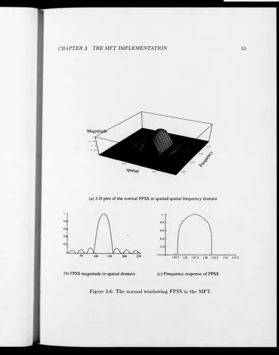
to forward transforms and inverse transforms respectively... 3.5 The analysis filters are disjoint for critical sampling scheme and over­ lapping 50% for the oversampling scheme... 3.6 The normal windowing FPSS in the M F T ... 3.7 The oversampled FPSS window... 3.8 The spatial implementation of the M F T ... 3.9 Exact reconstruction of the M FT using (3.17)... 3.10 The forward M FT implementation. (Note: M > N ) ...

3.12 The 2-D M FT is generated from convolution of analytic window spec­

trum with frequency shifted version of input signal... 64

3.13 A synthetic texture field and its M F T ’s at different resolutions. . . . 66

3.14 The FM-Radial test pattern and its M F T ’s at different resolutions. . 68

3.15 The reptile skin and its M FT’s at different resolutions... 70

4.1 Texture warping is modelled via affine transform... 74

4.2 Outline of algorithm... 76

4.3 Representative centroid vectors; A] is coordinates between (0j, +#2), A2 is coordinates between (#1 + #2. 0\ + 7r), /T) is centroid in Ai and /¿^ is centroid in A2... 78

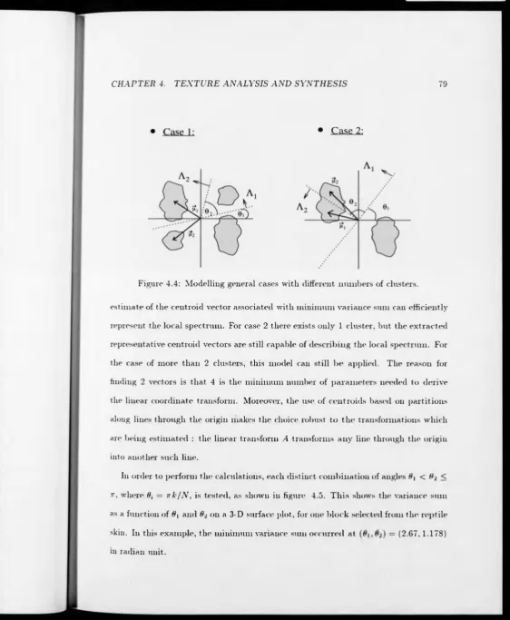
4.4 Modelling general cases with different numbers of clusters... 79

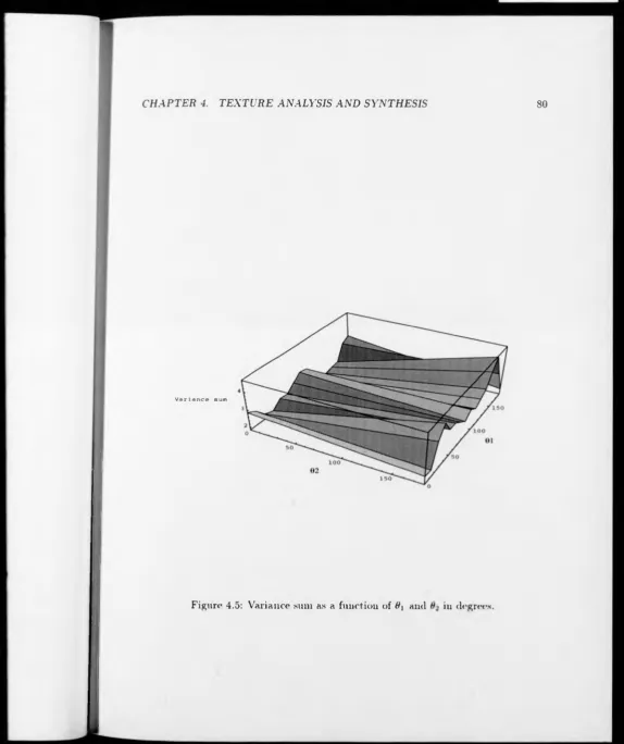
4.5 Variance sum as a function of 9\ and 82 in degrees... 80

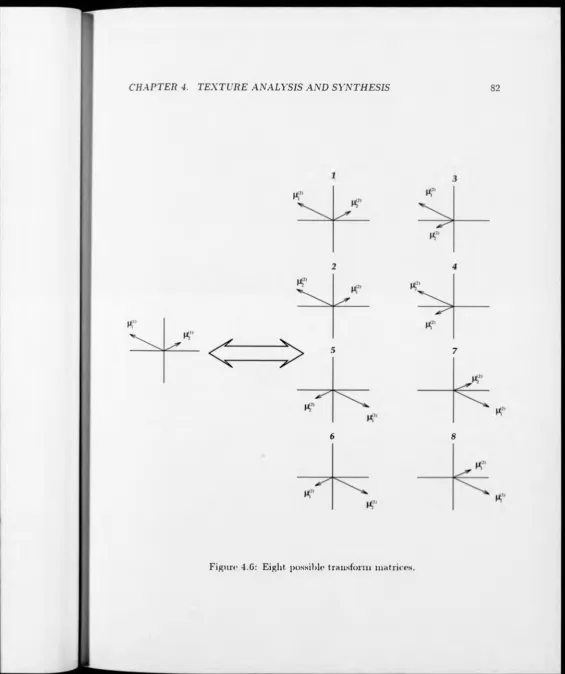
4.6 Eight possible transform matrices... 82

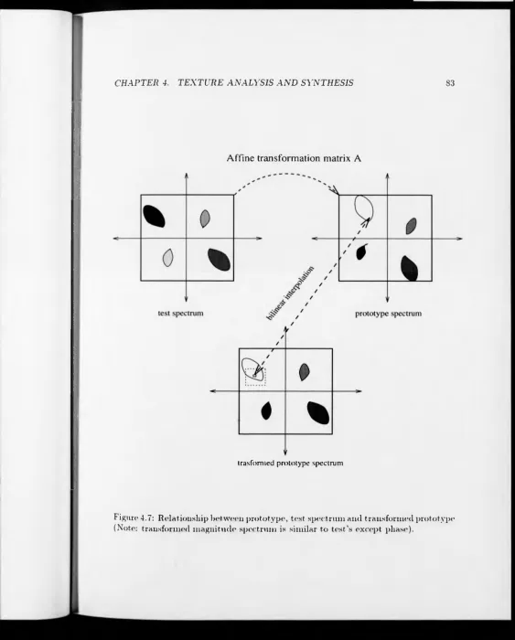
4.7 Relationship between prototype, test spectrum and transformed proto­ type (Note: transformed magnitude spectrum is similar to test’s except phase)... 83

4.8 Bilinear interpolation... 84

4.9 Correlation between prototype and the 8 transformed MFT blocks gives the best fit... 86

4.10 Reconstruction from the cosine square function... 89

4.11 Low pass portion removed in the beginning and combined with syn­ thesis result in the end, where a is the energy factor... 90

4.12 Lowpass image of the reptile skin reconstructed at M FT level 4. . . . 91

4.13 Relationship between the quality of synthesised image and the number of parameters used per pixel for synthesis... 92

4.14 FM-Radial Test Pattern and vector pair and the 8 possible spectra from the test block. The resynthesised prototype for each case is shown at the bottom right. Transform number 5 provides the best fit... 94

4.15 Natural textured image synthesised from a prototype... 97

4.16 FM-Radial test pattern and synthesis... 98

4.17 Reptile skin image synthesised at different levels... 101

4.18 Burlap image synthesised at different levels... 102

4.19 Grass image synthesised at different levels... 103

4.20 Normalised mean-square error as a function o f the number of parame­ ters used for synthesis... 104

O * O * O * C t O ' O i C n C i ü « C i C i O » O ’ O i ü i C n C n

horizontal direction; bottom figures show their amplitude spectra. . . 113

.2 Outline of the texture segmentation at single level...115

.3 One level of the orientation pyramid is created corresponding to the M FT block-based gradient operation... 119

.4 Boundary enhancement using 8 direct neighbour gradient vectors. . . 121

.5 Case where adjacent pixels have high region and boundary link prob­ abilities (cf. figure 5.15)... 123

.6 Consistency check among 4 neighbour gradient vectors against their father node... 125

.7 Synthetic structured texture pair... 128

.8 Synthetic random texture pair... 128

.9 Natural random texture pair... 129

.10 Natural structured texture pair... 129

.11 Synthesised colour reference map for orientation... 130

.12 Orientation pyramids of testing texture pairs, (a) Synthetic structured texture, (b) Synthetic random texture, (c) Natural random texture grass water, (d) Natural structured texture burlap reptile skin... 131

.13 Magnitudes o f orientation estimates correspond to those in figure 5.12. (a) Synthetic structured texture, (b) Synthetic random texture, (c) Natural random texture grass water, (d) Natural structured texture burlap reptile skin... 132

.14 Boundary estimate is enhanced via boundary link probability itera­ tively. (a) Boundary links at MFT block scale of size 16 x 16. (b) Boundary links after 3 iterations, (c) Boundary links at M FT block size 8 x 8 . (d) Boundary links after 3 iterations... 134

.15 Region connectivity is described via region link probability iteratively. 135 .16 The generating order of the segmentation results illustrated in the fol­ lowing figures (cf 5.17. 5.18 and 5.19)... 135

.17 Iteration results of orientation pyramid o f synthetic random texture. . 137

This work was supported by the Government o f the Republic of China on Taiwan and conducted within the Image and Signal Processing Research Group in the Department of Computer Science at Warwick University.

I would like to thank all the staff of the Computer Science Department. In partic­ ular, thanks go to all my friends and colleagues, past and present, of the Image and Signal Processing Group at Warwick: Abhir Blialerao, Simon Clippingdale, Nicola Cross, Andrew Davies, Wooi Boon Goh, Andy King, Peter Meulemans, Edward Pear­ son, Hugh Scott, Tim Shuttleworth, Martin Todd, and Horn-Chang Yang. They have made numerous contributions and have provided a stimulating environment in which to work. Thanks also to Jeff Smith for providing essential software support.

I would like especially to thank Dr. Andrew Calway for his enthusiasm and stim­ ulating discussions regarding to the work of texture synthesis.

I declare that, except where specifically acknowledged, the material contained in this thesis is m y own work and that it has neither been previously published nor submitted elsewhere for the purpose of obtaining an academic degree.

Introduction

1.1

Introductory Remarks

Texture is a ubiquitous property of visible surfaces, but there is no formal or pre­

cise definition of texture. The term ‘texture’ generally refers to repetition of some

elemental unit over a region which is large compared to that of the elemental unit

[54]. This element contains several pixels, whose arrangement may follow certain

rules, which may be periodic, quasi-periodic or random. A large class of textures can

be covered by such a definition, ranging from structural texture (reptile skin) and

random texture (grass) to crop imagery, as shown in figure 1.1.

Texture is one of the important characteristics which exists for analysis in many

types of natural images, from satellite imagery in remote sensing, to microscopic

images of medical samples, to outdoor scenes and object surfaces. The problem of

texture description centres around both what precisely is meant by ‘texture’ , for there

is a large number of attributes of texture that may be defined, and how such textured

regions should be generated and analysed.

1.1.1

Visual Texture Perception

Visual textures have great variability. How human beings perceive texture and what

the crucial factors are that affect the discrimination of two texture fields are two

important issues in deciding the characteristics o f what we see. A large amount

of experimental evidence has shown that for detection of visual stimuli, the visual

system behaves as if it were composed o f a number of independent channels, each

sensitive to a limited range of spatial frequencies and orientations [62] [47]. From the

psychological and physiological view [87], an important determinant in the detection

of the stimulus by the human visual system is its spatial frequency content.

Two hypothesised mechanisms of the human visual system for texture perception

are ‘texton’ detection and texture filtering. The first class of models reported by

Julesz et al [61] [60] regard the fundamental texture elements as textons, which are

used to describe features of individual sub-patterns that render texture pairs with

identical second order statistics discrim inate. Discrimination is accomplished by the

comparison of the relative texton densities, which is claimed to be consistent with

the visual discrimination o f textures. However, the difficulty in using this approach

to the segregation o f textures is that no suitable mechanism was proposed for local

extraction of textons or the texture boundary.

Among models o f texture filtering, Caelli [15] advocated a Fourier model which is

able to simulate the human visual system on the basis of mechanisms which decom ­

pose an image into its frequency components, including both amplitude and phase

coding. A set of ‘ clam sin’ll' filters centering on different parts of the Fourier domain

fields. While these efforts have demonstrated that a filtering approach can explain

some phenomena that are not consistent with texton theory, a complete model has

not yet been presented. Such a model should be able to unify the solution of the con­

flicting problems of determining local textural structures (texture element, texture

boundaries) and identifying the spatial extent of the textured regions contributing

significant spectral information.

1.1.2

Texture Analysis Problems

Most texture research can be characterised by the underlying assumptions made about

the texture formation process. These assumptions depend primarily on the type of

textures to be considered in the study. This leads to classification of the approaches for

texture analysis into either statistical approaches, considering the texture as defined

by a set of statistics extracted from a large ensemble of local image measurements,

or structural approaches, using the concept that a textured image is composed of

texture elements.

Statistical A p p ro a ch e s

The conventional statistical methods for texture analysis summarise the gray level dis­

tribution into a finite number of statistics, among them the well-known co-occurrence

matrices [51], [110]. These methods are based on the estimation of the second-order

joint conditional probability density function, f(i,j\ d , 0). Each f(i,j\ d , 0) is the prob­

ability of going from gray level i to gray level j , given the intersample spacing distance

d, and the direction given by the angle 0. The estimated values, x$(i,j\d), can be

occurrence matrices have been developed and their capability has been demonstrated

[23] [46]. In these methods, textural structures which can be described within a

neighbourhood are naturally limited to those which are observable within the size of

the neighbourhood. Thus a feature based on measurements within a neighbourhood,

fixed in size, has poor discrimination power when applied to a texture not observable

within the neighbourhood because it has the wrong scale. But in general the scale

information is not available. This is a fundamental limitation o f such methods.

Alternatively, a parametric model m ay be used for statistical modelling. The most

common stochastic models of texture are the autoregressive [58], or more generally

Markovian Random Field (M RF) m odels [25] [44]. Chellappa and Kashyap [18],

suggested the use of 2-D autoregressive, noncausal models for textures. In this model,

the gray level of a pixel is characterised as a linear combination of the gray levels at

neighbouring pixels and an additive linear combination of some noise field values. The

model parameters are estimated by approximating a maximum likelihood solution for

various possible neighbourhoods. One of these models is chosen, using a Bayesian

decision rule, to approximate the original noncausal model and then to synthesise

images. Chen [19] proposed a maximum entropy power spectrum estimation method,

which involves a parameteric way of estimating spectrum based on an autoregressive

model. These methods are widely used but are of limited applicability to images

because the causality restriction is significant: the autoregressive model is limited by

its inherent directionality, which introduces a degree of anisotropy.

An edge-based segmentation technique based on features derived from a simulta­

neous autoregressive (SAR) random field was described by Khotanzad and Chen [2],

of the windows, the least squares estimates of the SAR model parameters are used as

texture features. Texture edges in each window are placed at positions where sudden

changes in the features of a neighbouring window occur. Enhancement of individual

feature edges is carried out via a block-based 3 x 3 Sobel operator to produce an

initial edge map. The enhanced texture changes are combined to construct a ‘tex­

tural measure’ and thresholded to give a texture edge. This texture edge is further

thinned to give a one-pixel wide skeleton. It should be noticed that the accuracy of

the estimated edges is determined by the window, due to the use of block-based edge

detection. Although the result is thinned, significant misplacement may still occur

when an inappropriate scale of the window is used.

Stochastic image models based on the Gibbs distribution [45] are of great current

interest. In [31], Derin and Elliot use the Gibbs distribution for texture segmentation

via a dynamic programming method and maximum a posteriori (M A P ) criterion

which allows the use of standard least squares techniques iteratively. This work is

applicable only to noise-free textured images consisting of known textures and with

known Gibbs distribution parameters. This technique also requires a small enough

neighbourhood, so that equations can be determined for obtaining the least squares

solution.

Texture boundary detection incorporated by the introduction of a binary valued

line process described by Genian et al [44] is another notable use of this approach.

Two types of labels, partition and boundary labels, are used in a region partition

process and boundary detection respectively. The local blocks of the image in the

region process are augmented by line sites which are placed between each vertical and

include all possible pairs o f allowable block and line states. The distance between pairs

of neighbours is measured by the Kolmogorov-Smirnov distance and this is used to

detect discontinuities. Adopting the Gibbs representation, a form of energy function is

defined to place the boundary between regions and prohibit certain configurations that

are false edges or very small regions, resulting in a reduction of the number of model

parameters. Although the results shown are improved by introducing the line process,

the size of the line process neighbourhood is artificially set by the region assignment

process. As noticed in [1], in this modified MRF model, the model parameters cannot

be estimated by standard methods, such as maximum likelihood estimation, because

the solution of the likelihood equation compounds the problem of model parameter

identification, resulting in computational intractability.

Elfadel and Picard [36] examined a method which describes an explicit relation­

ship between co-occurrence matrices and Gibbs random fields. An intermediate rep­

resentation including an ‘ aura set’ and ‘aura measure’ is developed to establish the

connection with morphological dilation combined with co-occurrences. Based on the

concepts of the Gibbs energy and MAP estimation, the results of their method show

that their work is still in its initial stages.

More recently, the Gaussian Markov Random Field (G M R F ) [22], [21] and [17]

was applied in unsupervised texture segmentation. An image of interest is divided

into disjoint regions; over these regions the GMRF parameters are estimated. The

regions are merged via clustering based on the normalised Euclidean distance between

their parameter vectors. Following recomputing of the parameters over the merged

regions, a refined segmentation is carried out via pixel-based segmentation. The

One difficulty for these methods is that the texture elements in the stochastic

process are not highly structured and large data sets may be required to get good pa­

rameter estimates [83] [38]. In general, statistical methods are well suited to textures

which are random in nature, such as sand, grass and perhaps water, whilst textures

such as tilings of the plane, brick wall and reptile skin are not appropriate for this

type of model.

S tru ctu ral A p p r o a c h e s

Unlike the stochastic models, structural approaches have not received much attention

recently [51] [53]. They include the development of a compact structural description of

texture by the minimum number of parameters needed to identify the placement rule

of the texture elements [82], In general, these methods first locate texture elements,

then analyse spatial arrangements. In natural images, texture fields may be degraded

during imaging and obscured by noise and blur. Even with complete knowledge of

texture types, it is more difficult to isolate the texture elements than it is to generate

them.

Matsuyama et al [71] resolved this difficulty by first estimating a pair o f spatial vec­

tors from the Fourier energy spectrum representing the placement rule of the texture

elements. Then, following inverse Fourier transformation of the estimated vectors,

texture elements are extracted by a region growing method. The basic disadvantage

o f this method is its preliminary assumption of the completely periodic structure of

the texture field. The synthesis procedure is performed by placing ‘averaged' texture

elements according to the estimated placement rule, resulting in artificial looking

Similarly, the method described in Volet and Kunt [97] extracts the placement

rule first, based on a pair of linearly independent vectors derived from the local

autocorrelation function of the image. W ith the extracted placement rule, the texture

is transformed to a ‘normalised’ co-ordinate space via an affine transform and the

texture element is then extracted. A global average texture element is obtained by

averaging the normalised local texture elements and used with geometric warping in

order to reconstruct the image. McColl has applied this idea in texture coding [72].

Vilnrotter et al [96] examine the statistics of edge features to control texture ele­

ment identification and isolation. From the isolated texture elements, a set of place­

ment rules are computed. The reconstruction is performed by combining these into a

complete description. As in earlier structural methods, the results are acceptable only

in the case o f periodic textures. These structural methods have generally assumed

that the textures exhibit some degree of regularity, which is violated in many textures

[53].

S u m m a ry

Both of these types of methods depend highly on the texture type, which restricts

their applicability. Thus, while statistical techniques are generally good for random

textures and have poor performance on structural textures, the revers«* is the case for

the structural techniques. Ideally, a method which is capable of dealing with the full

spectrum of texture types is required.

Having defined textured images as composed of texture elements and rules which

describe the spatial arrangement of the texture elements, there are two basic questions

Texture element estimation is concerned with local property measurement. How­

ever, textures occurring in natural images generally show randomness or variability

and exhibit fluctuations, ranging from the degradations occurring in the image for­

mation process, surface irregularity and geometric warping caused by the 3-D to 2-D

projection. Inevitably, these intrinsic properties affect the local texture measures

used in analysis. Solutions often involve operations with local windows, which re­

quires choosing the windowing function and window size. Choosing the right scale is

a fundamental problem because texture is an area property [52]. There is seldom a

systematic basis for choosing the window size. If the window is too big, for example,

it may be difficult to identify region boundaries or adapt to variations within regions,

while if it is too small it may give unsufficient discrimination o f the textures.

Apart from the above problem, the windowing function prevents an image being

considered at arbitrarily high resolution in both spatial and spatial frequency do­

mains. This problem is a consequence of the uncertainty principle of signal analysis,

which states that the size of the regions of support of a windowing function in space

and frequency are inversely related - the smaller the window in frequency, the larger

will it be in space and vice versa [75] [108]. Uncertainty is a problem for any window

size used in spatial/spatial frequency representation. Daugman [28] shows that the

2-D Gabor function [40] can achieve simultaneous localisation in space and in spatial

frequency to resolve the uncertainty problem. A number of researchers have used Ga­

bor functions as filters to establish a scheme of multichannel filtering, which involves

the decomposition o f images into multiple feature images of narrow spatial frequency

and orientation bandwidth [9] [59] [92] and [34]. Some issues exist in these approaches

over, to tune each channel to a specific narrow band of spatial frequencies generally

requires prior knowledge, which is unlikely to be available in the unsupervised mode

of analysis.

In analysing the spatial arrangement of elements, it would be useful to find a

method which is intermediate between the random placement o f stochastic methods

and the rigid rules of the simple structural approaches. This requires a method which

has sufficient flexibility to allow for the sort of variation exhibited in the textures

shown in figure 1.1 and in which the scale of the description can be matched to that

of the texture elements.

Finally, segmentation of textured images requires location o f the boundaries be­

tween the textured regions. The task of boundary detection between textured regions

- texture segmentation - shares a common problem in vision, which Marr defines as

‘knowing what is where by looking’ [70]. ‘W hat’ is the element of texture, which

establishes the class property of the perceived image, while ‘where’ is the position

of the perceived texture in the spatial domain [108]. The main question in texture

segmentation regarding the texture properties and positions is raised by the fact that

identification of the texture type requires global information to yield a reliable de­

scription, which reduces the precision of the local boundary detection. Similarly, the

texture boundary can be detected more accurately only at the cost of a loss of relia­

bility of the classification. It implies that there is an incompatibility between texture

1.1.3

Aim s o f This Work

Central to the requirement o f a model which can both locally detect texture elements

and globally describe the density of the texture elements simultaneously, is the avail­

ability of a framework allowing the image to be considered at different scales and the

information at these different scales to be combined or compared. A solution to this

is to use a multiresolution approach (e.g. [85] [14] [109] [67] and [73]). A number of

workers have employed such techniques in texture analysis [78] [91]. More recently, a

classification scheme for texture analysis in the context of multiresolution imagery was

described by Roan et al [84], In this work, the statistical features were derived from

the Fourier energy spectrum and co-occurrence matrices to study the relationship

between feature properties and image resolution, which provides a useful approach in

textured surface description. Unser and Eden [95] used the output of a filter bank

to estimate local statistics of texture iteratively, giving a multiresolution sequence of

feature planes. A feature reduction technique was proposed, allowing variety textures

to be analysed in a single reduced component, but the problem of unsupervised deter­

mination of optimal window size remains unsolved. In [8], Bouman and Liu applied

a causal Gaussian autoregressive m odel to describe the statistics of the textures. A

coarse to fine segmentation was used in a multiresolution framework, requiring signif­

icantly less computation than earlier work using single resolution methods. Mao and

Jain [69] suggested a multiresolution simultaneous autoregressive model (M R-SAR)

for texture classification and segmentation. The method shows MR-SAR can achieve

a substantial improvement over the single resolution SAR model. The multiresolution

researchers and will be discussed more in Chapter 2.

To summarise, the objectives of this work are:

1. To investigate the characteristics of texture features.

2. To devise a technique which allows for the modelling of global image structure

in the same framework as that used for the local texture estimate, making com­

putation efficient, as well as providing a consistent interface between local and

global structure. This will allow analysis and synthesis of textures with varying

amounts of structure.

3. To create a boundary detection algorithm, which combines information of both

boundary position and texture properties at different scales and accommodates

neighbourhood information to achieve segmentation of textured images.

1.2

Thesis Outline

A multiresolution approach to the analysis of texture is presented in this thesis. The

multiresolution Fourier transform (M F T ) is used as a framework to derive a robust

algorithm which estimates textural features and detects texture boundaries over a

range of spatial scales, based on local frequency domain properties.

In particular, in Chapter 2, the requirements of an image texture description will

be discussed. The emphasis is piaceri on locality in representing the texture features.

A number of existing models which might provide such description are reviewed. How­

ever, evidence will be given that these fail to provide sufficient locality in describing

texture features. This leads to the modelling of the texture using the multiresolution

Chapter 3 is devoted to considering the definition and implementation of the M FT.

The MFT characteristics and properties will be discussed. T w o different interpreta­

tions of the MFT suggest two corresponding implementations. The implementations

can be accomplished efficiently using the FFT algorithm. Initial experiments and

examples are presented for both synthetic and natural images.

Chapter 4 introduces a new texture ‘synthesis and analysis’ algorithm based on

the MFT framework. This algorithm models textures by the use of affine co-ordinate

transformation of a single, representative texture element. It extends the earlier work

reported by Spann and Wilson [104] to model the structure in textures in a way

which allows for variation o f the texture structure. Results are presented o f texture

synthesis based on this approach.

In Chapter 5, a texture segmentation algorithm is described, which is designed

using a cooperative algorithm within the M FT framework. The detection of tex­

ture boundaries uses a combination of boundary information and region properties.

Results are presented that illustrate the effectiveness o f the scheme.

The thesis is concluded in Chapter 6 with a synopsis and a discussion of some

Representations for Texture

Analysis

2.1

Introduction

Texture can be used in image analysis in several ways, such as classification and dis­

crimination of surface patterns, computation of the geometric structure of perceptual

objects and segmentation of the scene into different homogeneous regions [108]. It

was shown in Chapter 1 that the analysis o f textures is one of the oldest problems

in image processing, but continues to generate interest and a degree of controversy

because of the limited success with which most of the methods of analysis have met

[51] [46] [83],

The purpose of this chapter is to present and evaluate the characteristics of differ­

ent texture analysis approaches which have been proposed, particularly the Fourier

related approaches. To overcome limitations in those approaches, a general signal

representation for texture analysis is set forth.

2.2

Requirements of a Texture Analysis Method:

The problem of obtaining useful texture measures is difficult because of the multi­

plicity of texture properties and their variation with parameters such as illumination,

shading and surface reflectance. There is the question o f finding an adequate descrip­

tion of texture - of selecting features which are sufficient to allow discrimination of

the types of texture encounted in a given application. Furthermore, the perspective

projection of 3-D textured surfaces into 2-D images causes distortions in the area,

orientation, shape and coarseness of the texture elements, and many natural textured

images exhibit a combination of regularity, such as approximate periodicity, and vari­

ation which is hard to model using either straightforward repetition or traditional

statistical techniques [51, 25, 112].

In order to find an adequate description of texture, it is possible to formulate

the requirements of a representation for texture analysis as linearity, invertibility,

symmetry and locality:

2.2.1

Linearity

Linearity can provide the conditions to ensure the predictable response of the pos­

sible addition and filtering operations on the signal. If the descriptor is linear, the

computation can be simplified and filtering operations can be more easily applied.

2.2.2

Invertibility

Image processing consists of a number of operations performed on the image. These

operations transform the original image to another feature space and in this trans­

ations usually cause a loss of information in passing from the original image to its

feature-space representation. Very often, the dimensionality of the feature-space is

lower than that o f the image space, and only an approximation o f the original image

based on this partial information is reconstructed. An invertible operation preserves

information, and in principle allows the original image to be recovered, while also

providing an error measurement between the approximation and the original image.

2.2.3

Sym m etry

The processes which produce the 2-D texture can in many cases be approximated

by affine transforms. These processes include the biological or mechanical process

by which the structure originated and the perspective transformation resulting from

the projection onto 2-D. The 2-D affine transform is a linear co-ordinate transform

followed by a shift and is given by

T (? ) = A £ + 7 (2.1)

where A is a matrix dealing with the rotation, scaling and shear, 7 is the translation

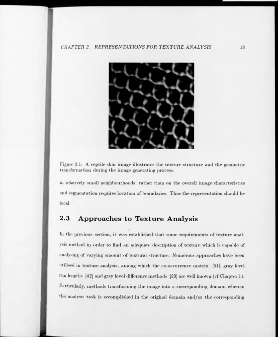
and £ is the co-ordinate. For example, in the reptile skin of figure 2.1 [11], the image

can be interpreted as a texture element associated with a geometric placement rule

which is approximately a 2-D affine transform. This geometric structure must be

embedded in the descriptor, which is the essence of symmetry.

2.2.4

Locality

Figure 2.1: A reptile skin image illustrates the texture structure and the geometric transformation during the image generating process.

in relatively small neighbourhoods, rather than on the overall image characteristics

and segmentation requires location of boundaries. Thus the representation should be

local.

2.3

Approaches to Texture Analysis

domain have received considerable attention in the literature [46] [83]. The purpose

of this section is to discuss and evaluate their characteristics.

2.4

Fourier Based Texture Analysis

Many of the traditional texture features have explicit interpretations in the frequency

domain such as ‘fineness’ corresponding to high frequency components, and ‘regular­

ity’ corresponding to peaks in the spectrum. Physiological and psychological evidence

suggest that the human visual system is capable of performing a form o f spatial fre­

quency analysis [29].

The chief properties of texture are periodicity and directionality, so that a suitable

texture analysis description has to be able to characterise these two features [15].

In Fourier analysis, a 2-D signal g ( x , y ) is decomposed into a linear combination of

complex exponential functions of the form eJ(-r"*+v--'i/) an(j w ith coefficients given by

% , « , ) =

J g(x,y)e-^-+^ )dxdy

2

2

The complex exponential has interesting properties. Consider the case

that for a given frequency co-ordinate (u>T,wy) and for some n

XijJjr + yu>„ = 2 7Til (2.3)

then

e+j(xM,+u^v ) _ e+j2irn _ j _(2.4)

In other words, the basis function with frequencies (uix,uju) is a wave in a specific

orientation, with a real part as in figure 2.2. From (2.3) we know that

<jjz 2mi

y

x +

That is, the slope of each line is — jj^, and the normal to all o f them is a line oriented

at an angle 0 = a rcta n (^ ). The spatial period (i.e. the distance between zero phase

lines) is given by

Thus the Fourier transform is a natural choice for texture analysis, which underlies

many of the methods described in the literature [4] [5] [37]. The Fourier transform

defined in (2.2) leads to a rich mathematical structure associated with the transform

operation. These mathematical properties such as linearity, invertibility and symme­

try have ensured that the Fourier transform provides a general texture representation.

In the aspect of locality, however, the Fourier transform has to be enhanced in order

to become a general texture analysis tool. This will be addressed in the following

sections.

In addition to the secure mathematical structure, the Fourier transform is conve­

nient for handling noise. If there is noise within the textural image, the noise process

will alter the image representation dramatically in the spatial domain, but uniformly

in the frequency domain. Hence, frequency domain measures should be less sensi­

tive to the noise than those in the spatial domain. Fourier based analysis is of most

relevance to this work. Traditional Fourier based texture analysis uses the energy

spectrum, which is the Fourier transform of the image autocorrelation function [75].

2.4.1

Autocorrelation Methods

Texture is an extended, spatially nonlocal or region property. Since texture is defined

in relation to a neighbourhood, it is meaningless at an isolated pixel. The relationship

suggests the autocorrelation function r(ra,n ) as a texture descriptor defined as

^ N - 1 N - l

rg(m, n ) = — J2 $(*> 0 » (" * + « + 0 (2.7) ■‘V *r=0 /=0

where m and n are known as the ‘lag’ . For the sake of efficient computation, the

autocorrelation may be calculated using Fourier transforms [75]. There are two types

of information contained in rg( m, n) . If the peak of the autocorrelation function

falls off quickly as the lag departs from zero, this corresponds to a finer texture. A

high-energy peak associated with rg( m, n ) for nonzero lag also reveals a regularity in

the spacing of texture elements in patterns such as wall paper. In terms of these two

useful texture measurements, the autocorrelation is able to measure the directionality

and coarseness of the texture.

The autocorrelation methods are based on spatial averages o f second-order inter­

actions. Methods which involve higher order statistics [41] require more memory

space and are computationally expensive. The autocorrelation function, however, is

not sufficient to describe a texture completely, since many natural textures have sim­

ilar autocorrelation functions. Furthermore, its estimation often requires a large data

window. In such cases, the description loses the locality of the texture identification

and the computational cost increases dramatically.

2.4.2

Energy Spectrum M ethods

Bajcsy [4] first used the Fourier energy spectrum to compute the sample energy

spectrum with radial and wedge segments in analyzing texture. She also reported

that phase information does not appear to yield useful texture measures. Rosenfeld

S

p

a

ti

a

l

frequency

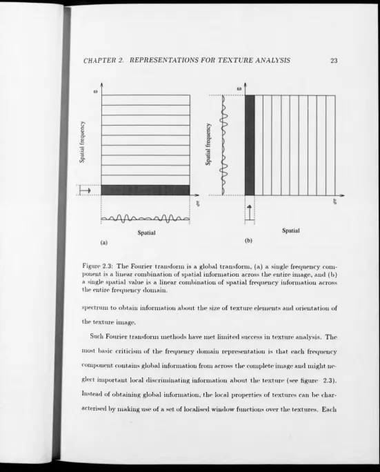
Figure 2.3: The Fourier transform is a global transform, (a) a single frequency com ­ ponent is a linear combination of spatial information across the entire image, and (b) a single spatial value is a linear combination of spatial frequency information across the entire frequency domain.

spectrum to obtain information about the size of texture elements and orientation of

the texture image.

Such Fourier transform methods have met limited success in texture analysis. The

most basic criticism of the frequency domain representation is that each frequency

component contains global information from across the complete image and might ne­

glect important local discriminating information about the texture (see figure 2.3).

Instead of obtaining global information, the local properties of textures can be char­

localised window function highlights a particular property of the texture element or

the response of the human visual system.

There are some difficulties associated with these measures:

1. The ring and wedge shaped functions used to com pute the texture features were

essentially a windowed Fourier transform (cf. section 2.5.1). Spatial locality is

introduced by windowing the data prior to the integration of the energy of the

transformed windowed data. However, this involves a loss in spatial frequency

resolution, as the spectrum of the image is now convolved with that of the spatial

window.

2. One consequence o f windowing is that it destroys symmetry under co-ordinate

transformations since windowing and co-ordinate transformations do not com­

mute. That is, some features of an image within a window might disappear after

co-ordinate transformation of that image. This raises the uncertainty problem

of signal analysis. Uncertainty will be a problem for any window size used in

spatial/spatial frequency representation (cf. section 2.5.1).

3. Coarseness in textural features is always scale dependent. This scale characteris­

tic should be resolved in the feature descriptor to allow the image to be analysed

at different scales. The selection of the appropriate processing scale is essen­

tially context-dependent. Some of the texture element extraction has assumed

that the processing scale is known a priori.

4. Feature information in both the spatial domain and frequency domain is required

2.5

Spatial and Spatial Frequency Methods

Combined spatial and spatial frequency representations are useful in classifying non-

stationary signals like textured images. Features which have identical or similar spa­

tial or spectral characteristics may have very different characteristics in the comple­

mentary domain, which allow them to be distinguished. In addition, physiological and

psychological experiments have shown that the human visual system processes visual

information at different frequencies separately and is highly orientationally selective

[37] [15]. For the purpose o f texture segmentation, perceptual grouping is dependent

on both the spatial and spectral structure. All these factors point to the need for high

resolution and a conjoint representation of the spatial and spatial frequency domains.

This conjoint representation is known as a phase-space representation [27].

Recently, then* has been much work based on phase-space analysis in which meth­

ods have become ever more sophisticated. Representations that provide information

about a texture locally over various scales have received considerable attention in

the literature. The best known of these approaches fall broadly into four classes:

windowed Fourier transform, scale-space transform, pyramid transform, and wavelet

transform.

2.5.1

Windowed Fourier Transform

The windowed Fourier transform (W F T ) is the best known of the methods which

provide intermediate representations o f the signal both in spatial and frequency do­

mains. The windowed Fourier transform or short-time Fourier transform (STFT) has

windowed Fourier transform of a discrete-time signal x(£) is given by

OO

£ ( £ > /) = — m ) x ( m ) e ~ j ™fm 0 < / < M (2.8) m = — oo

where w(() is a window function and ‘ ’ is used to denote the Fourier transform.

The WFT can resolve nonstationary signals which have distinct frequency content at

different instants into ‘quasi-stationary’ signals by windowing the input. The scale

of the window will decide the corresponding frequency resolution. To increase the

frequency resolution, one has to increase the size of the spatial window, which causes

nonstationarities which might occur within this duration to be blurred: the spatial

resolution decreases.

Ring and wedge shaped analysis windows discussed in section 2.4.2 are inherently

a windowed Fourier transform, but suffer from infinite spread in the spatial domain

because of the discontinuous windows used. One of the best known W FT methods

in image analysis is the Gabor transform [40]. The standard Gabor representation

is given by

x(£,u;) = f u>(£ — m)x(m)e~**m dm (2.9)

J — OO

where w({) is a windowing function, which in the original Gabor scheme is a Gaussian

function.

Denoting the windowing function, shifted in space and spatial frequency, as

= (

2

10

gives its Fourier transform as

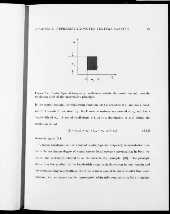
Figure 2.4: Spatial/spatial frequency coefficients within the resolution cell have the resolution limit of the uncertainty principle.

In the spatial domain, the windowing function w(£) is centered at and has a band­

width of standard deviation Its Fourier transform is centered at u>, and has a

bandwidth of <rw. A set of coefficients .r(£, to) is a description of ,r(£) within the

resolution cell of

[Î. - + 0{] x [u>, - (2.12)

shown in figure 2.4.

A major constraint on the conjoint spatial/spatial frequency representation con­

cerns the maximum degree o f simultaneous local energy concentration in both do­

mains, and is usually referred to as the uncertainty principle [40]. This principle

states that the product of the bandwidth along each dimension in one domain and

the corresponding bandwidth in the other domain cannot be made smaller than some

Hence, the resolution cell has to obey the inequality [40] [27]

^ (2.13)

Given this constraint, Gabor claimed that the Gaussian windowing function is a

suitable filter to provide maximum simultaneous locality in both spatial and spatial

frequency domains.

One approach, proposed by Spann and Wilson [104], uses the joint spatial and

spatial frequency space in texture analysis. A number of interesting and important

features reported in this work has motivated other image analysis work [102]. Jain

and Farokhnia [59] used even-symmetric Gabor filters to measure the local energy.

Du Buf [32] applied a least-squares approximation to measure the local Gabor energy

spectrum in terms of visually relevant texture attributes such as directionality and

coarseness. Bovik et al [9] used 2-D Gabor functions as localised filters to encode

images into multiple narrow spatial frequency and orientation channels. By analyzing

the responses of the filters, it was possible to segregate textural regions of different

spatial frequency, orientation or phase characteristics.

The Gabor representation provides a local description in the conjoint spatial/spatial

frequency domain, and preserves the symmetry property o f translation in the spa­

tial/spatial frequency domain. However, the spatial/spatial frequency resolution cell

is of fixed size, as is shown by applying the Fourier transform to equation (2.9) with

different frequencies; different cells have the same bandwidth but different spatial

frequency position. The limitation of a fixed resolution cell of the Gabor represen­

tation leads to the rectangular quantisation of the conjoint spatial/spatial frequency

____ exp[-x*x ]

. . . .cos(x)ex p[-x*x ]

____ cos(5 x )exp [-x*x ]

cos(7 x )exp [-x*x ] (0

(a) Garbor function with different modulation frequencies

/ \/ / A, / / \

/ / /

\ ;

O’

J

o. CO * y \

V A

/ !

Spatial

(b) Fourier transforms o f Gabor functions in (a) (c ) Tessellation o f spatial/spatial frequency

plane by Gabor functions

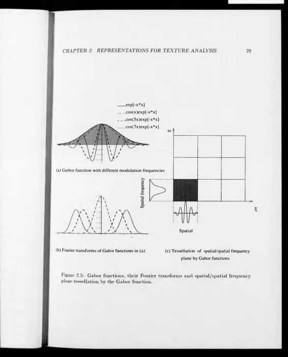
of three different frequencies and (b) shows the corresponding Fourier transforms.

That the Fourier transforms have the same shape but different positions indicates

that the Gabor function has a fixed bandwidth, (c) depicts the spatial/spatial fre­

quency plane tessellation in terms o f these elementary Gabor functions; note again

that the resolution cell is of fixed size and shape.

The local structure of a texture is hard to characterise by a single scale. An im­

portant requirement of such representations is that over the range of possible features

the locality in each domain should not be fixed. The texture features should have

various degrees of locality and extend over different sized areas of the other domain.

In order to combine locality at various scales, a multiresolution framework has to

be used in the analysis. Multiresolution approaches can be divided into scale-space

methods and hierarchical frameworks.

2.5.2

Scale-space Representation

In a scale-space representation, a signal is convolved with Gaussian functions of in­

creasing width. For the signal f ( x ) , with scale <7, spatial co-ordinate £, the scale-space

representation is defined as

(2.14)

where

<7 (2.15)

is the filter kernel. Marr [70] used image features at different resolutions to represent

an image. By matching zero-crossing locations of second derivatives through these

on these estimates, the image can be segmented into primitive regions upon which

object recognition may be performed. Within applied similar ideas to propose a scale-

space filtering function [109]. This method is based on smoothing the signal with

a filter of continuously increasing scale. The resulting blurred signal is processed

by a second derivative operator. This is equivalent to convolution with the second

derivative of the Gaussian function, given as

where a is the standard deviation o f the Gaussian function. Koenderink has developed

the scale-space representation further into a general approach to vision [64]. Its main

weaknesses for texture are that it is computationally expensive and does not provide

a natural set of features for analysis.

2.5.3

Pyramid Representation

Normally, a given image and particularly a textured image will have different structure

at different resolutions. A pyramid representation of an image uses a hierarchy o f

regularly spaced resolution levels [79]. Images of different resolution are formed by

lowpass filtering, then subsampling to the new Nyquist frequency. At the top level

of the pyramid is the most lowpass version of the image, which may be as small as

l x l . At the bottom level of the pyramid is the image of the highest resolution - the

original image. A basic pyramid representation can be used in image decomposition

and is defined as a function of a logarithmic scale [85], as follows

M M

* ( 6 , 6 , 0 = £ £

wU, k)x (2^- j , 2i 2 - k , l - l )

where / denotes the scale and w(£i,£2) is a lowpass kernel defining the transformation

function between the different scales. The pyramid representation has been applied

to different fields of image analysis and particularly coding because most of the image

energy is contained in the high levels of the pyramid, which have fewer pixels. Burt

[12] has defined a multiresolution representation consisting of regularly spaced resolu­

tion levels. He has applied the transform to many aspects of machine vision including

texture analysis. Larking and Burt [65] computed local energy spectral estimates

upon each of the bandpassed image of the multiresolution bandpass transform, and

pixels are classified by energy to perform texture segmentation. Burt [13] suggests

the use of edge density instead o f spectral density as a texture measure.

Multiresolution pyramid processing is computationally effective, especially for low

level image analysis. The computational advantage of performing processing on sev­

eral resolution levels has been studied in detail by Rabiner et al [24]. The main

difference from the windowed Fourier transforms is that in a pyramid, the frequency

domain is split into regions having constant relative bandwidth. That is, the ratio of

bandwidth to centre frequency is fixed, whereas in the windowed Fourier transform

the tessellation is in terms of absolute bandwidth. Figure 2.6 show's a pyramid repre­

sentation where each square in the frequency plane is the region corresponding to one

basis vector. The pyramid representation is invertible and deals properly with scale.

In order to process structural differences over scale, the pyramid representation [14]

utilised the multiresolution framework to extract the difference information between

the approximation of an image at two different resolutions [85]. The extraction of

the difference is a bandpass filtering function, and Burt and Adelson called this a

resem-□

Pyramid frequency plane Spatial tessellation window

bles the action o f Laplacian-of-Gaussian bandpass filters [14]. The Laplacian of the

lowpass Gaussian filter is an isotropic function. In such cases, the transform not only

removes the possibility of introducing bias but also reduces the artefacts caused by

the rectangular nature of the sampling grid. On the other hand, because it is an

isotropic function, the Laplacian-of-Gaussian bandpass filter has restricted utility in

estimating orientational features. Moreover, the Laplacian pyramid representation

is overcomplete, because the whole representation contains 4/3 times the number of

samples in the original image, all of which are needed for the perfect reconstruction.

2.5.4

Wavelet Transform

The wavelet transform is a signal representation which decomposes the signal by

expanding the signal into a family of functions having the same bandwidth on a

logarithmic scale, obtained by the dilation and translation of a unique function the so

called motherlet. In the 1 — D case, the wavelet transform o f a signal f ( x ) is defined as

= ~7= f f ( x ) w ( - — - ) d x (2.18)

\J (7 J (7

where u>(£) is the wavelet function, which satisfies some admissibility conditions [49].

The 2-D discrete wavelet transform originates from the Laplacian pyramid. The

simplest discrete wavelet transform coefficients are derived by successive decimation

and translation operators, using one lowpass filter li and one highpass filter </ to

retain the same sample count as that of the original image. Since the decimation will

introduce aliasing terms, the general trend so far has been to seek an orthogonal set

is a pair of quadrature mirror filters defined in terms of the Z-transform as [100]

G(z) = - z - ' H i - z - 1) (2.19)

where G (z) and H(z) are the Z-transforms of the lowpass and highpass filter respec­

tively. In this manner, the aliasing terms caused by the subsampling will be cancelled

so that exact reconstruction can be achieved and the redundancy of the representation

minimised.

The wavelet frame can be well localised in both time and frequency domains. In

phase-space, their time/frequency spread is low and they have good conjoint resolu­

tion. Therefore, by representing a signal with such bases, each coefficient corresponds

to the magnitude of the motherlet at that location (in time or frequency). The discrete

wavelet transform is fast to compute, using a tree-based algorithm.

The basic concept of using two filters in the wavelet transform is that the high-pass

filter is used to extract ‘ details’ at a given scale, while the low-pass filter is used to

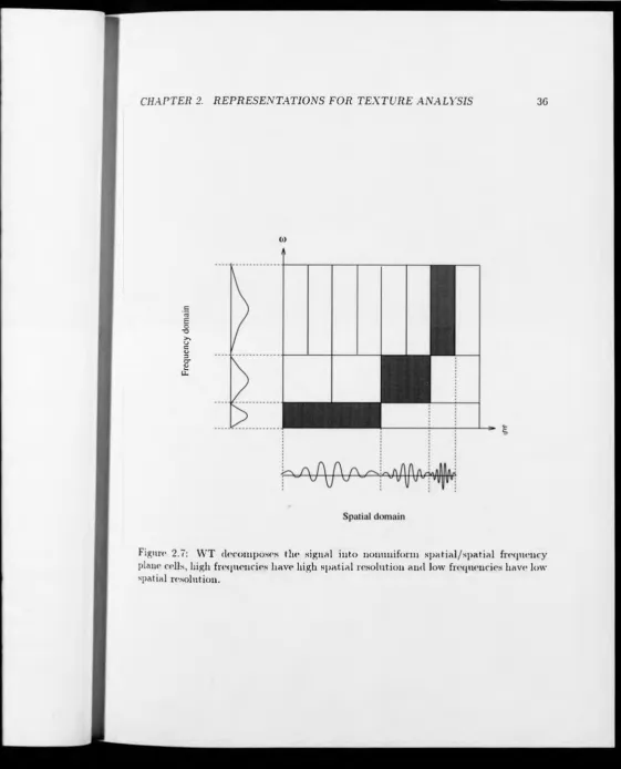
smooth the signal to allow the next scale to be explored. As an illustration, figure

2.7 demonstrates the tessellation of the conjoint spatial/spatial frequency domain by

the wavelet transform. The spatial co-ordinate £ and spatial frequency co-ordinate u>

m the wavelet transform are related in such a way that cells at high frequencies have

low frequency resolution and vice versa. Further reading ran be found in Daubechies

[26] and Mallat [67].

The conventional wavelet transform appears not to possess a rich enough basis to

give a general way of modelling and analysing images. This is because each scale

m a 2-D wavelet transform contains only 4 frequency bands [100]. An alternative

F

req

uen

cy d

o

m

a

in