1
Data-Driven Retail Food Waste Reduction
A comparison of demand forecasting techniques
and dynamic pricing strategies
Paula Felix
Master Thesis
August 2018
Preface
First of all, I would like to thank the members of my graduation committee, Klaas Sikkel, Fons Wijnhoven and Maurice van Keulen, for guiding me in this 9-month thesis writing process and for all your valuable feedback. I really enjoyed our meet-ings and always left motivated to continue and improve my thesis. In addition, I would like to thank my Deloitte colleagues for giving me the opportunity to write my thesis there, for their useful suggestions and of course for making my time at the office so enjoyable. Handing in this thesis officially marks the end of my time as a student at the University of Twente and these five years as a student have really flown by. Although I won’t be a student anymore, I hope to continue to learn many new things and be challenged on a daily basis in my future career.
Executive Summary
Every year one third of all food that is produced is wasted and one of the UN sus-tainable development goals is to cut food waste in half by 2030. This thesis focuses on two data-driven strategies to reduce perishable food waste at retailers: demand forecasting and dynamic pricing. Improved demand forecasting techniques can pre-vent excess inpre-ventory by better supporting replenishment decisions, whereas dynamic pricing can reduce excess inventory once it exists by stimulating customers to buy older products at a discount. The performance of both traditional and promising new demand forecasting techniques is compared and implementation guidelines are provided for retailers. In addition, simulations were conducted to investigate the performance of different (dynamic) pricing strategies in terms of revenue, waste and stock-outs. For retailers, reducing perishable food waste results in financial and sustainability benefits.
Demand Forecasting
Demand forecasting techniques that were included in the performance evaluation are: naive (where the forecast equals sales from last period), exponential smoothing (ES), moving average (MA), linear regression (LINREG), auto-regressive integrated moving average (ARIMA), support vector regression (SVR), multi-layer perceptron (MLP), long-short term memory network (LSTM) and adaptive boost (ADA). These techniques were evaluated based on their performance in forecasting sales for 986 perishable food products from an Ecuadorian supermarket. Performance was mea-sured using the relative root mean squared error measure (RelRMSE), which is a robust measure that indicates how well a certain technique performs relative to the naive forecast. Performance was compared across different forecasting scenarios, which differed in terms of their time detail level, location detail level and horizon. In addition, it was investigated what the influence is of using external factors such as the weather in addition to historical sales data to produce forecasts.
Results show that there is no such thing as the ultimate demand forecasting technique and that performance greatly varies across products and forecasting sce-narios. By far the best demand forecasting performance overall can be obtained by automatically selecting the best forecasting technique for each individual product, resulting in (depending on the forecasting scenario) a 6% to 32% RelRMSE improve-ment compared to always using the naive forecast and a 2% to 10% improveimprove-ment compared to always using the best individual demand forecasting technique. Adding external factors from the weather, promotion, economic and holiday categories has shown to be valuable for forecasting scenarios that have a daily time detail level, enabling an additional 3% to 9% RelRMSE improvement compared to using
4
ical sales data only. For each forecasting scenario, detailed results and an overview of the top 3 best performing individual techniques are provided in this thesis to help retailers select the appropriate demand forecasting technique(s) in their situation.
In addition, a process is provided with step-by-step guidelines for retailers on how to improve the wider demand forecasting process. It not only considers how to select the right demand forecasting technique(s), which form the quantitative core of the demand forecasting process, but also discusses how to assess forecasting capabilities and which qualitative factors should be taken into account, such as implementation in decision support systems, adoption factors and organizational factors.
Dynamic Pricing
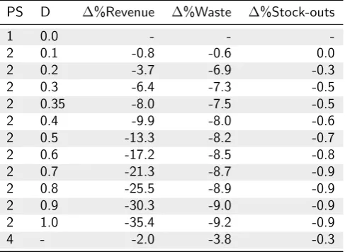
A simulation study was conducted to determine which (dynamic) pricing strategy for perishable products performs best in terms of total revenue, waste and stock-outs. The simulation considers a monopolist grocer selling a single perishable product with a fixed shelf life. The product can be replenished each day based on the demand forecast and a safety factor. Customers have different characteristics: some customers are regular customers that only pay attention to price, whereas others are date-checking customers that also pay attention to remaining shelf life and aim to choose a product that maximizes their value-for-money. Four main pricing strategies for marking down perishable products that approach their expiry date were compared. Strategy 1 applies no price changes at all and serves as a baseline. Strategy 2 applies a fixed discount D at the last day before expiry, while strategy 3 spreads that discount over the last S days before expiry. Strategy 4 dynamically determines discount percentages based on the demand forecast and the remaining inventory.
Almost all strategies that applied a discount resulted in a waste reduction, but they regularly resulted in significantly lower revenues. Multiple experiments were conducted to investigate the effects of varying assumptions for simulation settings. Discounting was most beneficial when product demand was more elastic and when more customers checked expiry dates, because that resulted in higher waste reduc-tions and less negative (or even positive) changes to revenue at the same time. The fixed pricing strategy that most frequently performed best was strategy 2 with a fixed discount of 20% on the last day before the expiration date. Surprisingly, the dynamic pricing strategies did not always perform better than a fixed price strategy, which could be due to the fact that these strategies relied upon imperfect demand forecasts and hence their estimated optimal discount percentage might have been off base. A dynamic pricing strategy already outperformed the best fixed strategy when initial waste levels for a product were high or when a large percentage of customers were regular customers.
Conclusion and Discussion
5
such excesses by discounting products that approach their expiration dates. Grocers are advised to follow the demand forecasting improvement process, to use this study as a benchmark for forecasting technique selection, to implement multiple forecasting techniques and to automatically select the best forecasting technique for each product. To resolve any excesses that do occur in stores, grocers are advised to use the pricing strategy that showed best performance in similar situations in the simulations. The best fixed strategy in general is applying a 20% fixed discount on the last day before expiry. A dynamic pricing strategy only outperformed a fixed strategy in a few situations.
Contents
Preface 2
Executive Summary 3
1 Introduction 9
1.1 Introduction to Demand Forecasting . . . 9
1.2 Introduction to Dynamic Pricing . . . 10
1.3 Benefits for Food Retailers . . . 10
1.4 Problem Statement . . . 11
1.5 Research Questions . . . 11
1.6 Thesis Structure . . . 12
I
Enhancing the Demand Forecasting Process
13
2 Demand Forecasting Background 14 2.1 Forecasting Problem Dimensions . . . 152.2 Qualitative Forecasting Techniques . . . 15
2.3 Quantitative Forecasting Techniques . . . 17
2.3.1 Time Series . . . 17
2.3.2 Smoothing Techniques . . . 17
2.3.3 Regression . . . 18
2.3.4 ARIMA and Variations . . . 19
2.3.5 Neural Networks . . . 19
2.3.6 Ensemble Techniques . . . 20
2.3.7 External Factors for Demand Forecasting . . . 21
2.4 Forecasting Performance Evaluation . . . 22
2.4.1 Performance Measures . . . 23
2.4.2 Evaluation Procedures . . . 24
2.5 Forecasting in a Retail Context . . . 24
3 Research Method 27 3.1 DF Problem Scenarios Considered . . . 27
3.2 DF Techniques Evaluated . . . 28
3.2.1 Evaluation Measures and Procedure . . . 29
3.2.2 Hyperparameter Tuning . . . 29
3.3 Dataset and Preparation . . . 30
CONTENTS 7
3.3.1 Sales History Data . . . 30
3.3.2 External Factors Considered . . . 31
3.3.3 Data Preprocessing . . . 32
4 Performance Comparison Results 33 4.1 Results for One-Step Ahead Scenarios . . . 33
4.2 Results for Multi-Step Ahead Scenarios . . . 37
4.3 Results for External Factors . . . 40
4.4 DFT Comparison Conclusion & Discussion . . . 45
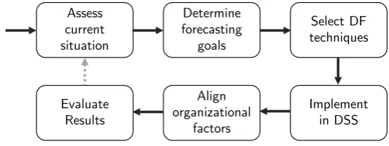
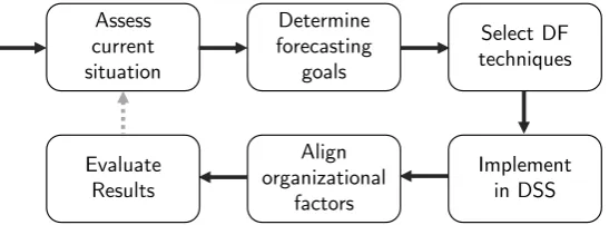
5 DF Improvement Process 48 5.1 Step 1: Assess Current Situation . . . 49
5.2 Step 2: Determine Forecasting Goals . . . 49
5.3 Step 3: Select DF Technique(s) . . . 49
5.4 Step 4: DSS Implementation and Adoption . . . 51
5.5 Step 5: Align Organizational Factors . . . 52
5.6 Step 6: Evaluate Results . . . 53
5.7 Conclusion and Discussion . . . 54
II
Dynamic Pricing of Perishable Food Products
55
6 Dynamic Pricing Fundamentals 56 6.1 Pricing Strategies . . . 566.2 Dynamic Pricing Problem Dimensions . . . 58
6.3 Related Work . . . 59
7 Research Method 61 7.1 Simulation Method . . . 61
7.2 Problem Formulation . . . 62
7.2.1 Pricing Strategies to Evaluate . . . 63
7.2.2 Performance Measures . . . 63
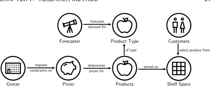
7.3 Simulation Model Components . . . 64
7.4 Model Assumptions . . . 66
7.4.1 Customer Arrival Rate . . . 66
7.4.2 Customer Behaviour Assumptions . . . 67
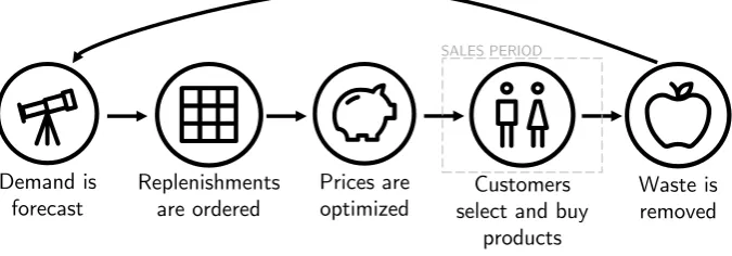
7.5 Walkthrough of a single simulation period . . . 68
7.6 Simulation Settings . . . 69
7.7 Experiments and Goals . . . 70
8 Simulation Results 72 8.1 Results Experiment 1: Default Settings . . . 72
8.2 Results Experiment 2: Shelf Life Variations . . . 73
8.3 Results Experiment 3: Regular Customer Probability Variations . . . 74
8.4 Results Experiment 4: Elasticity Variations . . . 75
8.5 Results Experiment 5: Safety Factor Variations . . . 76
8.6 Results Experiment 6: Sales History Variations . . . 76
CONTENTS 8
III
Conclusion and Discussion
80
9 Conclusion and Discussion 81
9.1 Results Summary . . . 81
9.2 Contributions . . . 84
9.3 Validity . . . 85
9.4 Suggestions for Future Work . . . 86
Appendices 92 A DFT Implementation Specifics 93 A.1 Package Use . . . 93
B DFT Evaluation Significance Tests Results 94
1
Introduction
Each year around one third of all food that is produced is wasted, which equals 1.3 billion tonnes and is worth around $1 trillion [25]. One of the UN sustainable development goals is to cut food waste in half by 2030 [63]. Food retailers such as grocery chains are in a unique position to contribute to this goal. They handle large quantities of food in their distribution centres and stores and are closely connected to both suppliers and consumers.
The food waste hierarchy [48] provides a framework for food waste reduction and shows 5 distinct stages: prevent, reuse, recycle, recover and dispose. Solutions that fall in the prevention stage are most favourable [48]. Two promising directions for reducing food waste in grocery chains using data analytics are enhanced demand forecasting (DF) and dynamic pricing (DP). Both directions fall in the prevention stage of the food waste hierarchy. Better demand forecasting can prevent surplus inventory, whereas dynamic pricing can reduce a surplus once it exists.
1.1
Introduction to Demand Forecasting
The goal of demand forecasting is to predict demand for individual products as accurately as possible to support business decisions such as replenishment. Inaccu-rate forecasts have been identified as one of the main causes for food waste at the retailer level [43]. So by improving the DF process, replenishment decisions can be better supported and surplus inventory can be prevented.
At the core of the DF process lie the forecasting techniques that are used, which can be qualitative, quantitative or a combination. The quantitative DF techniques are the main focus of this study. Qualitative techniques include expert opinion and the Delphi method. Traditional quantitative techniques include exponential smoothing (ES) and auto-regressive integrated moving average (ARIMA). Advances in predictive analytics have given rise to many new DF techniques over the last years. Newer methods for quantitative demand forecasting include variations of neural networks and ensemble methods. Various external factors can be taken into account as well, ranging from the weather and search trends to more general economic factors. Before selecting a forecasting technique, it is important to get insight into the characteristics of the forecasting problem at hand. Forecasts can differ on multiple dimensions, including the forecast horizon and the level of detail in terms of time, product and location.
CHAPTER 1. INTRODUCTION 10
It is important to realize that DF is about more than the techniques used, since the goal of DF is to support business decision-making. DF techniques are often im-plemented as part of a decision support system (DSS). Such a forecasting support system (FSS) can automatically create forecasts for products and aid employees in adjusting these forecasts if necessary to help them decide on replenishment quanti-ties. For DF implementation it is also important to consider organizational factors, such as processes and management practices surrounding demand forecasting, since those can also influence adoption and performance.
1.2
Introduction to Dynamic Pricing
The field of dynamic pricing focuses on finding the optimal product prices over time to maximize profit for the seller. The adoption of dynamic pricing has increased considerably over the last years, mainly due to the increased availability of internal and external demand data, the rise of technologies that make it easier to change prices and the development of decision support systems [20]. A traditional appli-cation area of dynamic pricing is the airline industry [13], where there is a fixed capacity (limited number of seats in an aircraft) and ticket prices are dynamically adjusted based on the marginal value of remaining seats.
Even though dynamic pricing traditionally focused on the airline and hospitality industries, it also holds great potential for food retailers since they face fluctuating demand over time and their product offerings include perishable products like fresh foods that lose their value after a certain expiry date. Dynamic pricing strategies can help food retailers to minimize waste when a surplus occurs. Dynamic pricing and demand forecasting are interrelated. Dynamic pricing models use demand forecasts, in addition to other data such as current inventory levels, to determine what price strategy is optimal for an individual product to minimize waste and maximize profit. In turn, the adjusted prices again influence customer demand.
1.3
Benefits for Food Retailers
Retailers operate in a challenging industry with heavy competition, relatively low margins and fluctuating consumer demand. The large variety of products on offer in their stores includes perishables, which decline in quality over time and expire after a certain date, resulting in shrink (lost inventory value). Fresh food items are very important for grocers since they account for up to 40% of their revenue [39] and can be responsible for 80% of the total store shrink [47]. Hence reducing perishable product waste will improve retailer profitability.
One success story comes from Tesco, a large food retailer in the United King-dom. Their improved DF system saved£100 million a year and a DP system for marking down perishable products further reduced waste by 2% a year and saved an additional£30 million each year [29].
CHAPTER 1. INTRODUCTION 11
Another benefit of enhanced DF for retailers is improved on-shelf availability, since forecasting inaccuracy is one of the root causes of stock-outs [18]. If a prod-uct is out-of-stock, this may result in opportunity cost due to missed sales oppor-tunities. In addition, stock-outs have a negative effect on customer satisfaction and especially when a customer faces stock-outs multiple times, there is a high chance that that customer will go to a different store [18]. So retailers do not just have to prevent surplus inventory, but they also have to prevent stock-outs to keep customers satisfied.
1.4
Problem Statement
With one third of food going to waste each year, it is clearly an issue that has a big impact on our society. Cutting food waste in half by 2030 is one of the UN sustainable development goals. To contribute to achieving this goal, food retailers have to reduce the waste from their distribution centres and stores. For most, it is already part of their sustainability agenda for the coming years.
With the increasing digitization of the industry, opportunities arise for retail com-panies to implement advanced demand forecasting techniques and dynamic pricing strategies to reduce food waste. Many new forecasting techniques are developed in literature but their adoption in practice lags behind. It is difficult for companies to decide which DF technique to implement because a wide variety of techniques exist and new variations are published frequently. To the best of our knowledge, there is currently no thorough comparison of the performance of demand forecasting techniques for food retailers and practical guidelines for implementation are lacking. The potential of dynamic pricing to reduce waste also remains unclear so far and hence retailers would benefit from a simulation comparing the benefits of different pricing strategies.
1.5
Research Questions
Following from the introduction and the problem statement, the following main research question has been formulated for the thesis:
“How can enhanced demand forecasting and dynamic pricing contribute to reducing food waste at the retailer level?”
Separate sub questions have been formulated for the demand forecasting (DF) and dynamic pricing (DP) parts of the research.
DF1. Which quantitative demand forecasting technique performs best in fore-casting perishable product demand?
DF2. What guidelines can be provided to improve the wider forecasting process in practice?
CHAPTER 1. INTRODUCTION 12
varied as well, specifically one- versus multi-step performance, weekly versus daily forecast performance and store- versus country-level performance will be evaluated. In addition, the added value of including external factor data on top of historical sales data will be examined. Since overall forecasting performance depends on more than just the technique used, question DF2 provides guidelines on how to improve the wider forecasting process aspects including decision support systems (DSS) and organizational factors.
DP1. What (dynamic) pricing strategies can be used for the sale of perishable food products in supermarkets?
DP2. What simulation model can be used to simulate perishable food product sales in supermarkets?
DP3. In simulations, which pricing strategy performs best in terms of total revenue, waste and stock-outs?
For question DP1, dynamic pricing strategies will be developed that optimize per-ishable product prices over time. Fixed pricing strategies will be discussed as well. For question DP2, a simulation model will be developed and assumptions will have to be made about consumer behaviour. The impact of different pricing strategies on revenue, waste and stock-outs will be evaluated using simulation experiments to answer question DP3.
1.6
Thesis Structure
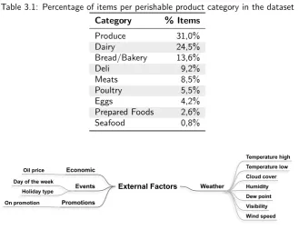
The remainder of the thesis roughly follows the research questions in its structure and is divided into three parts. Part 1 covers demand forecasting, part 2 covers dynamic pricing and part 3 discusses results and draws conclusions. Figure 1.1 gives an overview of the structure of the thesis. Within part 1 and part 2, relevant background literature is covered to provide all readers with a solid background on both topics. Readers in a hurry who already have sufficient background knowledge can decide to skip these chapters without it limiting their ability to understand the rest of the thesis.
Chapter 2
Chapter 6 Chapter 7 Part II
Chapter 3 Chapter 4 &5
Chapter 8
Chapter 9 Background Research Method
Part I
Results
Part III
Part I
Enhancing the Demand
Forecasting Process
2
Demand Forecasting
Background
The purpose of this chapter is to provide readers with a background on demand forecasting and to introduce the wide variety of forecasting techniques that are described in literature and used in practice. The goal of forecasting is to make predictions about the future value of variables and to do that as accurately as possible to support business decision-making. Section 2.1 describes the different dimensions of forecasting problems.
Figure 2.1 gives an overview of the main classes of forecasting techniques. On the highest level, forecasting techniques can be split into qualitative (section 2.2) and quantitative techniques (section 2.3). Qualitative techniques include expert opinion, the Delphi method, prediction markets, surveys and scenario development. Quantitative techniques can be further split into simple smoothing techniques tion 2.3.2), regression techniques (section 2.3.3), variations of ARIMA models (sec-tion 2.3.4), neural networks (sec(sec-tion 2.3.5) and ensemble techniques (sec(sec-tion 2.3.6). Section 2.3.7 discusses the variety of external factors that could be used as exten-sions to some of these DF techniques to further improve performance. Section 2.4 discusses forecasting performance measures and evaluation procedures. Section 2.5 provides context of demand forecasting in the grocery sector by reviewing available literature and discussing current practices at one large Dutch grocer.
Qualitative Quantitative
Demand Forecasting Techniques
Smoothing Regression (S)ARIMA(X) NetworksNeural Ensemble
Figure 2.1: Types of forecasting techniques
CHAPTER 2. DEMAND FORECASTING BACKGROUND 15
Figure 2.2: Overview of demand forecasting dimensions
2.1
Forecasting Problem Dimensions
Before selecting a forecasting technique, it is important to get insight into the characteristics of the forecasting problem at hand. Forecasts can differ on multiple dimensions, of which figure 2.2 gives an overview.
The forecast horizon dimension and aggregation on the dimensions of time de-tail, location detail and product detail account for the largest differences between forecasts. Depending on the sector of the company for which the forecast is cre-ated and the decision that is supported, the forecasting problem has its own unique characteristics.
One dimension is the forecast horizon. With single-step forecasting a prediction is made for a single future period, while multi-step forecasting predicts values for two or more future periods. Aggregation on three different dimensions also results in different forecasting problems. Aggregation can occur on the time detail, location detail and a product detail dimensions. The time detail of a forecast can for example be monthly, weekly, daily or even sub-daily (e.g. hours or minutes). The appropriate time detail level depends on the forecasting needs. For example in energy sector, a sub-daily demand forecast is crucial, whereas for car sales forecasting a monthly forecast might be enough. On the product detail dimension, forecasts can be created on a category level, subcategory level, individual item level (style) or even at the stock-keeping unit level (e.g. different sizes of each style). On the location detail dimension forecasts can be created country-wide, per region, per distribution centre or per individual store. The lower the aggregation level (so the more detailed the forecast) and the longer the forecasting horizon (more steps ahead), the more complex the forecasting problem is and the harder it is to make accurate forecasts.
2.2
Qualitative Forecasting Techniques
Qualitative forecasting techniques are subjective ways to produce forecasts. Qual-itative techniques can be helpful in situations where there is limited availability of historical data, for example with the introduction of new products. With the most basic qualitative forecasting technique, a domain expert decides on a forecast based on his experience, intuition and any information about external factors that he/she knows might influence demand.
CHAPTER 2. DEMAND FORECASTING BACKGROUND 16
provides a process for multiple experts to state and combine their forecasts. In mul-tiple rounds, experts create individual forecasts with argumentation and a facilitator anonymously reads all of them. This way, forecasters can adjust their forecast based on other experts’ arguments and the forecasts are likely to converge. After the last round the forecasts are combined and through this process the final forecast will likely be less biased than when one forecaster would have made a single forecast.
Prediction markets also aim to combine the knowledge of multiple participants. In a prediction market, forecasters trade contracts with a pay-off that depends on the outcome of uncertain future events [60]. Market prices represent the aggregated expectations of the forecasters about for example demand for a new product.
Another technique that is frequently used is market research, where surveys are sent out to consumers to gauge their demand for certain products as well as to get an idea of what factors influence their demand. Teschner and Weinhardt [60] provide a comparison of prediction markets and surveys, which shows that surveys are less complex, but that prediction markets provide continuous forecasts and enable forecasters to react to events. It is not clear yet whether prediction markets outperform other qualitative techniques, as research so far has produced mixed results [60].
Foresight literature describes several other qualitative techniques for long-term forecasting to support strategic decision making. Foresight is “the systematic pro-cess of looking into long-term future of science, technology and innovation” [33]. These techniques could support retailers’ strategic decisions such as assortment planning. With scenario development, multiple scenario stories are developed that each depict a different possible future. So these scenarios take into account dis-ruptions that might occur in the market. Roadmapping is another technique for strategic future planning where a visual chart is created that depicts developments from a technological, product and market perspective over time [49]. This can help retailers to assess the impact of market developments and new technologies.
A disadvantage of qualitative techniques is that because the techniques are sub-jective, the forecasts are susceptible to a number of human biases. It was shown that a forecaster’s personality and motivational orientation have a significant effect on forecasting biases [21]. For example, conscientiousness increases overreaction bias and anchoring bias, whereas openness to experience increases optimism bias [21]. With anchoring bias, forecasters rely too heavily on the information that was offered first (the “anchor”). With overreaction bias, forecasters react dispro-portionally to new information. Optimism bias refers to forecasters consistently overestimating. Mellers et al. [42] also found that forecasting performance can differ between individuals and that the top performing forecasters, so called “su-perforecasters”, maintained high performance over time and for a wide variety of topics (within geopolitical event occurrence probability forecasting). Superforecast-ers’ high performance can be explained by their cognitive abilities and styles (high fluid & crystallized intelligence), their task-specific skills (high scope insensitivity & forecasting granularity), their high motivation & commitment and their enriched environments (they could discuss with other superforecasters) [42].
CHAPTER 2. DEMAND FORECASTING BACKGROUND 17
2.3
Quantitative Forecasting Techniques
This section gives an overview of the main quantitative forecasting techniques. Be-fore diving into individual techniques, section 2.3.1 provides an introduction to time series since that is the main data source for all quantitative techniques. Then section 2.3.2 introduces simple smoothing techniques, section 2.3.3 regression techniques, section 2.3.4 variations of ARIMA, section 2.3.5 neural networks and finally section 2.3.6 introduces ensemble techniques.
2.3.1
Time Series
Time series are “a set of observationsy, each being recorded at a specific timet” [8]. The observations are sequential and have equal time intervals. Time series can be either univariate or multivariate, depending on the number of variables observed at each time t. One example of a univariate time series is ‘car sales revenue per month’, since it provides sequential values of a single variable (revenue from car sales) with a monthly time interval.
A time series can be decomposed into a trend component, seasonal component and residuals. The trend represents a long term growth/decline, whereas the sea-sonal component describes a recurring pattern over time. The residuals are what remains when the original data is detrended and deseasonalized.
In statistics each observationyt is viewed as a realization of a certain random
variable Y, so one important aspect of time series analysis is selecting a suitable probability model for the data. A general approach for statistical time series mod-elling consists of these steps [8]: plot the time series and examine the main features of the graph, remove the trend and seasonal components to get stationary residuals, choose a model to fit the residuals, forecast the residuals and invert the transfor-mations done in earlier steps to arrive back at forecast of the original series.
Demand exists when a customer appears who wants to buy a certain product or service. In forecasting, sales are frequently used as a proxy for demand. While this is reasonable in most situations, it is important to realize that when stock-outs occur too frequently or for longer periods of time, it is no longer an accurate approximation since there would be customers with demand who can not make a purchase. Throughout the rest of the thesis, the terms sales and demand are used interchangeably unless indicated otherwise. Sales forecasting can be considered a time series forecasting problem, since historical data is available on sales per time period.
2.3.2
Smoothing Techniques
The naive forecasting technique is the most basic way to produce forecasts. This approach takes the observed value from the previous period and returns that as the forecast for the next period(s). This is often used as a baseline to compare the performance of more advanced forecasting techniques.
CHAPTER 2. DEMAND FORECASTING BACKGROUND 18
Table 2.1: Overview of smoothing techniques
Technique Calculation
NAIVE Ft=Yt−1
MA Ft=∑qi=1Yt−i/q
ES Ft=αYt−1+ (1−α)Ft−1
Another smoothing technique is exponential smoothing (ES), which also takes the average of previous periods but places a higher weight on the observations from the most recent periods. The weights for older periods are decreased gradually using a smoothing parameter α, which lies between 0 and 1. The closerα is to 1, the more emphasis is placed on the most recent observations. Table 2.1 shows how to use these techniques to produce a one-step ahead forecast.
2.3.3
Regression
Regression analysis is a technique that aims to fit a line through observations of a variable Y using explanatory variablesXi. In general a linear regression model
looks like this:
Y =α+β1X1+...+βnXn+ϵ
where αis the intercept, β are the weights for each of the explanatory variables and ϵ is the residual term. Regression analysis produces estimates of α and the regression coefficients β. With linear regression a straight line is fitted through the observations. Polynomial regression is more flexible, since it can fit a curved line through the observations, in this case the explanatory variables in the formula notation above would have increasing powers.
Multiple regression analysis methods exists, including ordinary least squares, ridge and lasso regression. Ordinary least squares selects the regression coefficients in such a way that it minimizes the sum of squares of differences between the true values and the predicted values. Additional variants were developed to increase the predictive accuracy of regression models. With ridge regression, a maximum is imposed on the sum of the absolute regression coefficient values and coefficient values are lowered if necessary. Similar to ridge regression, lasso regression also imposes a maximum value on the sum of the absolute values of the regression coefficients, but when that value is exceeded coefficients are not only lowered, but can also be set to zero. To summarize the difference: ridge regression can reduce the impact that irrelevant explanatory variables have on results, whereas lasso regression can cut out those features completely.
CHAPTER 2. DEMAND FORECASTING BACKGROUND 19
2.3.4
ARIMA and Variations
One of the traditional time series forecasting techniques is autoregressive integrated moving average (ARIMA) [8]. Forecasts are based on an ARIMA(p,d,q) model. Parameter p is used for the model’s autoregressive (AR) component, which is a linear regression using the p previous values of the time series itself. Parameter d represents the level of differencing that is applied to the original time series and generally gets the value 0, 1 or 2. Let Y be the regular time series and Y′ the differenced series. With d = 0 no differencing is applied at all (Yt′ = Yt), with d= 1the first difference of the series (Yt′=Yt−Yt−1) is used and withd= 2the
second difference (Yt′ = (Yt−Yt−1)−(Yt−1−Yt−2)). Parameter q is the number of
lags for the moving average (MA). The MA component is a linear regression using the previous q random error terms. The ARIMA model can then be represented by the following equation:
Yt′=c+ϵt+ p ∑
i=1
γiYt′−i+ q ∑
i=1 θiϵt−i
The optimal values for p, d and q can be estimated by examining the auto-correlation function (ACF) & partial auto-auto-correlation function (PACF) plots. The ACF plot shows how correlated the data is with itself at different time lags [8]. At lags greater than q, the ACF plot should not be significantly different from 0. The estimation of parameter p is analogous, but then using the PACF plot instead of the ACF plot. The PACF plot is similar to the ACF plot, but also adjusts for the correlation values in between the two times of the lag [8].
It is important to note that ARIMA (and its variations) requires a stationary time series, which means that the mean as well as the variance of the series should be constant over time [8]. Stationarity can be tested with the Augmented Dickey-Fuller (ADF) test. If this test fails, the time series’ stationarity can be improved by employing a transformation technique. These transformation techniques either em-ploy some form of smoothing, like moving average (MA) or exponential smoothing (ES), or some form of differencing. Another constraint is that the ARIMA process assumes the time series has a zero mean [8]. If that is not the case, the time series can be made compliant with this requirement by subtracting the mean from each of the time series values.
Variations of the ARIMA model include SARIMA and (S)ARIMAX. Seasonality in the time series can be taken into account using SARIMA. The SARIMA model has 4 additional parameters: (P, D, Q) describe the seasonality and m represents the number of periods in each season. With (S)ARIMAX additional external factors can be taken into account, by adding aβiXifor alliexternal factors to the standard
(S)ARIMA model equation. The time series of the external factors have to comply with the same requirements, so it has to be stationary and have a zero mean.
2.3.5
Neural Networks
CHAPTER 2. DEMAND FORECASTING BACKGROUND 20
they can generalize and therefore also produce forecasts for previously unseen items. Thirdly, ANNs can approximate any continuous function and their functional forms are more general and flexible than those of other methods. Finally, ANNs are non-linear, which is often the case for real world systems. However, linear models have the advantage that they are less complex and easier to explain. There are several varieties of ANNs, of which the multi-layer perceptron (MLP) is one of the most commonly used. With an MLP, the first layer receives external input and the last layer produces output (a prediction in our case). Between these layers there are multiple hidden layers with processing nodes. These hidden nodes receive a number of input values, apply weights to them and then apply a certain activation function before outputting a new value to the next layer. An MLP is feed-forward, meaning that data is processed through the network in one direction. Some studies implement recurrent neural networks (RNNs) instead, which contain a feedback loop such that information can persist in the network and for example previous outputs could be used as inputs again. One RNN type that is suggested to be suitable for time series forecasting is long short-term memory (LSTM), which has the benefit of being able to learn long term dependencies. To go into some specifics, the main reason why LSTM has this ability is because it solves the vanishing (and exploding) gradient problems. For a detailed explanation of LSTM architecture, readers are referred to the original paper by Hochreiter and Schmidhuber [31].
Another variation of a feed-forward ANN is the extreme learning machine (ELM), which is tailored for bigger datasets. ELM is a new algorithm for training a feed-forward neural network with one hidden layer [67]. It has similar results as traditional ANNs but is much faster (up to 6 orders of magnitude).
ANNs require quite some hyperparameter tuning. There is a lot of flexibility in the number of hidden layers, hidden nodes, activation functions and learning algorithms. Two measures that are frequently used to determine the optimal pa-rameters are the Bayesian Information Criterion (BIC) and the Aikake Information Criterion (AIC) [50]. These information criteria help to select the model with the best fit, while penalizing model complexity. When comparing the AIC or BIC for two models, the model with the lower AIC or BIC is better than the other. Since AIC and BIC are relative measures, their value for just one model does not have any value. Similarly, AIC and BIC can also be used to automate the parameter selection for (S)ARIMA [8]. In addition to parameter tuning, the input parameters for the neural network have to undergo pre-processing, including a transformation to numeric values and scaling to be within a fixed range.
2.3.6
Ensemble Techniques
CHAPTER 2. DEMAND FORECASTING BACKGROUND 21
Figure 2.3: Overview of external factor categories with examples
2.3.7
External Factors for Demand Forecasting
When using (S)ARIMAX, regression or neural networks techniques for forecasting several external factors can be taken into account in addition to the historical time series data. A wide variety of external variables can be considered and their relevance could depend on the forecasting problem dimensions. The external factors can be grouped into several categories: weather, events, economic, promotions, product, competitors, social media, search trends. See figure 2.3 for an overview of these external factors. Some of these factors have a causal relationship with demand, for example in case of the weather (more umbrellas will be sold when it’s raining). Other factors, such as search trends, may merely correlate with sales (possibly with a lag). These factors are called ‘external’ because they are not directly about demand. It does not necessarily mean they are external to the retailer, since the promotions and product factors are within the retailer’s control (the other factors are not).
Weather-related factors that could be included in the model are: temperature, rainfall, sunshine hours or the deviation of those factors from the normal values at that time of year. It is expected that this factor has a causal relationship with the demand of some products, for example when it’s raining there will be more demand for umbrellas and when there’s a lot of sunshine BBQ products will be more popular. However, there will also be products for which sales are not influenced by the weather (e.g. toothpaste).
Event factors include all factors that make certain days stand out, including: day of the week, month, holidays (e.g. Christmas), school holidays (e.g. spring break), sports events (e.g. world cup games) and all other events (e.g. carnaval). It is expected that the event factors have a causal relationship with the demand of some products, for example when there’s a world cup game sales of beer and chips may rise.
CHAPTER 2. DEMAND FORECASTING BACKGROUND 22
necessity products (e.g. bread).
Promotion factors include factors that increase the attractiveness or visibility of a product. This includes advertisements, discounts and product placement. Product placement can influence sales because customers tend to buy those products that they see at eye-height or that are easy to grab. So for example when there is a special stand with products near the cashier, the products on that stand might have increased sales.
Competitor factors track competitor activities that might influence demand. Such factors can include discounts at the competitor, saving programs (when certain gifts can be earned) and special promotion periods with exceptionally good deals. A great deal at the competitor might directly negatively affect sales for a retailer due to customers switching stores or brands.
Product factors include the price, price relative to similar products, time in assortment and quality. Substitutes and complements of the product could also be included as external factors, since a rise in the demand of one product might cause a decrease in that of another (in case of substitutes) or cause a simultaneous increase in the sales of another product (in case of complements).
With the increasing popularity of social media and search engines, new data sources have become available to use in forecasts. Social media factors that could be considered include: number of mentions for a particular product or brand, number of retailer mentions and sentiment of posts about products/brands. Examples of search factors that could be included are the relative search volume for a product/brand and the difference in those search volumes per region. Social media and search factors might be correlated with sales with a time lag, due to the fact that people search for a product some time before buying it and might evaluate it on social media after buying it. For car sales, it was found that Google search trends and forum data have a significant effect in improving forecast accuracy [27] and that sentiment of social media posts has little further predictive value [66]. It was found that search trends and forum data had the most beneficial effect on forecasts for lower value car brands [27]. Another relevant concept is product involvement, which represents customers’ interest in a product and their perceptions regarding its importance and the perceived risk associated with it. Cars are a high-involvement product, so further research could examine the predictive power of these factors for low-involvement products like groceries and movies [27].
In conclusion, this section showed that there is a wide variety of external fac-tors that could be taken into account in demand forecasting. It is likely that the predictive power of these external factors might differ depending on the forecasting problem dimensions and even on the characteristics of the specific products forecasts are generated for.
2.4
Forecasting Performance Evaluation
CHAPTER 2. DEMAND FORECASTING BACKGROUND 23
Table 2.2: Overview of performance measures (adapted from [32])
Name Short Type Calculation
Mean absolute error MAE A mean(|et|)
Mean squared error MSE A mean(e2t)
Root mean squared error RMSE A √mean(e2
t)
Mean absolute percentage error MAPE P mean(|pt|)
Root mean squared percentage error RMSPE P √mean(p2
t)
Mean relative absolute error MRAE R mean(|rt|)
Geometric mean relative absolute error GMRAE R gmean(|rt|)
Mean absolute scaled error MASE S mean(|qt|)
2.4.1
Performance Measures
A wide variety of forecasting performance measures is available and on a high level they can be classified into four main types: absolute, percentage, relative and scaled [32]. Absolute measures are scale-dependent, while percentage, relative and scaled measures are scale-independent. A benefit of scale-independent measures is that they are easier to compare across different forecasts. This is especially helpful when there is a difference in the orders of magnitude of different forecasts, for example when one item is sold much more often than another.
The first step to measure performance is to determineet, which is the difference
between the observed value (Yt) and the forecast value (Ft) at timet. Percentage
measures usept. Relative error measures compare performance to a benchmarketb,
which is generally the naive method. Scaled error measures useqtwhich scales errors
using the in-sample MAE from the naive method [32] (the calculation provided forqt
is now for a one-step ahead forecast, similar calculations can be made for multi-step ahead forecasts).
et=Yt−Ft pt= 100∗et/Yt
rt=et/etb
qt=
et
1
n−1
n ∑
i=2
|Yi−Yi−1|
Table 2.2 (adapted from [32]) gives an overview of the most commonly used fore-casting performance measures and how they can be calculated.
There is quite some discussion about the suitability of different performance measures. An extensive, critical review of the available forecasting performance measures can be found in the paper by Hyndman [32], where the MASE performance measure was introduced as well. A survey of forecasters in the US showed MAPE is the most popular performance measure in practice [38]. One point of criticism on popular measures like RMSE and MAPE is that outliers can strongly influence the error calculations [24]. A problem with percentage errors is that they are undefined when there are observations with a value of zero. A deficiency of relative error measures is that etb can be small [32]. Another option would be to use relative
measures (e.g. RelM AE=M AE/M AEb) instead of relative errors, however that
CHAPTER 2. DEMAND FORECASTING BACKGROUND 24
Figure 2.4: Rolling Origin and Rolling Window Procedures
does not have these problems, since it is scale-independent, always defined and symmetric. This discussion indicates that RelRMSE and MASE are two of the most robust performance measures. They are also easy to interpret, since they indicate how well a certain technique performs compared to the naive method. For example, a RelRMSE<1 means that on average that technique gives smaller errors than the naive method.
2.4.2
Evaluation Procedures
The traditional procedure to evaluate forecasting techniques splits the available time series data into two parts, where the model is trained on the first part and evaluated on the last. However, this procedure does optimally use the available data. By doing cross-validation, a more generalizable impression of model performance could be obtained. With regular, k-fold cross validation, the data is split into k parts. When k = 5, the model is trained on 4 parts and evaluated with the remaining part, which is repeated 5 times so all parts have once been the test part. However, regular cross-validation is not a suitable approach in this case, since the data values are not independent. Because sales data is a time series, there is a temporal order in the values. Hence sales data will most likely violate the independence and identically distributed (i.i.d.) assumptions required for cross-validation.
Tashman [58] discusses several evaluation procedures that are tailored to time series forecasting. The forecast origin is the last data point the model uses to compute a forecast. During evaluations, the forecast origin can be fixed, in which case just a single forecast is computed, or rolling. A rolling evaluation procedure can have a rolling origin or rolling window. With a rolling origin the size of the training set differs over time, whereas the size is constant for a rolling window approach. Figure 2.4 illustrates this difference. For the rolling procedure, a choice has to be made between re-calibrating and updating. With re-calibration approach the model is re-trained for each step, whereas this is not the case with updating.
2.5
Forecasting in a Retail Context
CHAPTER 2. DEMAND FORECASTING BACKGROUND 25
Table 2.3: Overview of demand forecasting research with retail cases
Paper Sector Period Forecasting Techniques
ES MA Regression ARIMA(X) SARIMA(X) ANN Ensemble Other
[16] G D X X X XRBF X
[54] G D X XMLP
[11] G D XELM
[51] G W X X
[67] F M/Q/A X XELM, ENN
[52] F M X X X
[56] F M XELM
[53] F W X XELM XGM, PPD
[22] F H X X
[61] F Y/W X X X XANFIS
[27] A M X XMLP X XSVM
[66] A M X
[45] CE W X X XMLP, NARX
[19] CE M XMLP XANFIS
[4] O W X X X X X XANFIS
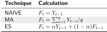
The majority of demand forecasting research with a retail case was focused on the fashion industry [67, 52, 56, 53, 22, 61]. For forecasting sales for a variety of fashion items it was shown that the ELM with a harmony search algorithm performed best [67]. In forecasting 5 different types of footwear, Ramos et al. [52] showed that state space models (including exponential smoothing) had a similar performance as ARIMA, so that neither can be said to be best for all circumstances. One paper completely focused on comparing different neural network variations [56] and found that ELM had the best performance & stability compared to two other backpropagation algorithms. Another paper [53] forecast the sales for 6 different fashion items and concluded that their developed pure-panel data (PPD) method performed best, followed by ELM and ARIMA, and that a grey model forecasting technique performed worst. Ferreira et al. [22] focused on forecasting hourly sales at an online fashion outlet called Rue La La and jointly optimizing the sales prices based on the demand model. A study with a large sample of 322 fashion items found that an adaptive network-based fuzzy inference system (ANFIS) had the best performance for forecasting both weekly and yearly sales [61].
CHAPTER 2. DEMAND FORECASTING BACKGROUND 26
regression (ensembles) and showed that multi-variate regression performed best [51]. Their external factors included price, holidays, discounts, inventory and regional factors. Besides demand prediction, the paper also focussed on price optimization. In a comparison of different ES variations for forecasting 256 grocery items, it was found that exponentially weighted quantile regression (EWQR) with just the constant factor performed best [59]. EWQR is equivalent to simple exponential smoothing of the cumulative distribution function.
Other papers had a case in the automotive [66, 27], consumer electronics [45, 19] or furniture sector [4]. The studies with a case in the automotive sector focused mainly on the predictive power of social media data and search trends as external factors and their results have been summarized in section 2.3.7. One of those papers mentions finding similar results for regression, ANN, SVM and ensembles [27], however the results of some techniques (SVM, random forest) were not included in the paper. For forecasting refrigerator component sales, it was found that a Non-linear Autoregressive Network with eXogenous inputs (NARX) had the best performance compared to traditional methods [45]. However, the authors used a limited sample and did no cross-validation. ANFIS was found to have the best performance for predicting sales of cash registers [19], based on a limited sales history and a simulation of additional data. For forecasting sales for 10 furniture items it was found that ensemble methods performed best [4]. Contrary to the most other forecasting literature, Aras et al. [4] did not find a statistically significant difference between the performance of ANN and other techniques such as ES and (S)ARIMA. From the overview in table 2.3, it becomes clear that even within the retail indus-try studies have different characteristics. The forecast period differs per sector, with the grocery sector mainly creating forecasts for sales per day, whereas other sectors generally have forecasts with a weekly or monthly time detail level. In addition, a wide variety of forecasting techniques is applied, but there is not yet one technique that stands out in terms of performance for forecasting retail sales. Table 2.3 shows that researchers have a focus on neural networks techniques (included in 11 out of the 15 reviewed studies), that smoothing (4 studies) and regression techniques (4 studies) receive considerably less attention and (S)ARIMA(X) somewhat less (8 studies). It is difficult to do a direct cross-paper comparison of results, since all pa-pers used a different dataset, slightly different variations of forecasting techniques with different external factors, different performance measures and some studies had a limited sample. However, when roughly generalizing the results it seems to point towards neural networks and ensembles as the best performing techniques.
The M3 competition [37] is also worth mentioning here because of its relatively large scale (3003 time series) and the large variety of DF techniques that was evaluated simultaneously. However, it does not focus specifically on retail sales, in fact the majority of time series were of different types, such a demographic time series. Almost no time series were considered with a daily or weekly time detail level, which further limits the usability of these results for retailers.
3
Research Method
The following two sub questions were formulated for the DF part of the research:
DF1. Which quantitative demand forecasting technique performs best in fore-casting perishable product demand?
DF2. What guidelines can be provided to improve the wider forecasting process in practice?
This chapter discusses the research method that was followed to answer these ques-tions. Sections 3.1 to 3.3 relate to question DF1 and the literature review process for question DF2 is shortly discussed in this chapter introduction.
For question DF1 the performance of different DF techniques was evaluated across different forecasting scenarios using perishable product sales data from an Ecuadorian food retailer (Favorita Corporacion). Section 3.1 describes the forecast-ing problem scenarios that were considered. The implemented DF techniques are described in section 3.2. Section 3.2.1 discusses the chosen performance measures and the followed evaluation procedure.
To answer DF2, a structured literature review was conducted. The wider fore-casting process aspects that will be investigated include forefore-casting evaluation frameworks, implementation of DF techniques in decision support systems (DSS) and their adoption, organizational factors influencing forecasting performance and criteria for DF technique selection. The goal of this literature review is to also include ‘softer’ aspects of the forecasting process and to develop a framework that guides the implementation of the quantitative DF techniques in practice.
3.1
DF Problem Scenarios Considered
To gain insight into which forecasting method is best in which situation, the fore-casting problem dimensions will be varied. The following forefore-casting dimensions will be considered:
• Forecasting Horizon: One-step (O) vs. multi-step (M) ahead forecast
• Time Detail Level: Weekly (W) vs. daily (D) level
• Location Detail Level: Country (C) vs. store (S) level
CHAPTER 3. RESEARCH METHOD 28
This results in 8 different scenarios: OWC, OWS, ODC, ODS, MWC, MWS, MDC and MDS. Within the multi-step ahead scenarios, there are again several variations depending on exactly how many steps ahead is forecast. All scenarios will be eval-uated with a 2-step ahead forecast (M2). The 3-step (M3) to 7-step (M7) ahead forecasts will be evaluated only for the DC scenario to limit the time needed for the evaluation. Additionally, two variations of input data for the DF techniques will be evaluated:
• Input Data: Historical sales only vs. external factors included
These scenarios are common in practice. The literature review and interviews showed that a weekly and daily forecast level is most common in the grocery in-dustry. At least one large Dutch grocer has the desire to move from a weekly to a daily forecast detail level. That same grocer has a multi-step ahead forecast (7-weeks ahead), but the one-step ahead forecast is most important and used for operations. Country-wide forecasts can be used to plan operations in distribution centres, whereas store level forecasts can be used for store-specific replenishment orders.
3.2
DF Techniques Evaluated
Several quantitative DF techniques were selected to be evaluated in this study based on the literature review and interviews. These techniques were selected for comparison:
• Naive, which is used as a baseline for comparison
• Moving average (MA)
• Exponential smoothing (ES)
• Auto-regressive integrated moving average (ARIMA)
• Linear Regression (LINREG)
• Ensemble - ADABoost of Linear Regression (ADA)
• Support Vector Regression (SVR)
• Neural networks (NN)
– Multi-layer perceptron (MLP)
– Long short-term memory (LSTM)
This selection represents traditional, commonly used techniques as well as new, increasingly popular techniques. Several of these techniques have been used in previous research, as could be seen from section 2.5, but to the best of our knowledge they were never evaluated simultaneously on a large sample. A survey by McCarthy et al. [38] (from 2006) gives an indication of how familiar forecasters (from the US) are with these techniques: forecasters were most familiar with moving average (84%), exponential smoothing (76%) and regression (73%), whilst they were least familiar with neural networks (17%).
CHAPTER 3. RESEARCH METHOD 29
details on how the individual demand forecasting techniques were implemented in Python. Specifically, appendix A.1 gives an overview of which functions / classes from which packages were used as a basis for the implementation of each of the demand forecasting techniques.
Section 3.3.1 describes the dataset that was used and provides some context on the company that provided it. Section 3.3.2 describes the external factors that were considered. Section 3.2.2 describes the set-up of each of the demand forecasting techniques and covers how the parameters for each technique were tuned.
3.2.1
Evaluation Measures and Procedure
Based on the discussion from section 2.4.1, it became clear that RelRMSE is one of the most robust forecasting performance measures. The fact that this is a scaled measure is useful for this study since performance will be compared across many product sales time series which may differ in magnitude. In addition, it allows for an easy comparison of the performance of different techniques compared to the naive forecast baseline. An RelRMSE<1 means that the particular technique on average performs better than the naive forecast. Percentage errors are unsuitable in this case because there will be days with zero sales for some products, particularly when looking at sales in individual stores.
The raw data was split into a training and a test set for evaluation purposes, where the training set contained 80% of the data available. As discussed in section 2.4.2 the regular k-fold cross-validation approach is unsuitable in this case due to the sequential nature of time series data. From the evaluation procedures that were proposed by Tashman [58] the rolling origin procedure was chosen for this study. The rolling approach makes optimal use of the available data and provides more robust performance results since it creates multiple forecasts. Since recalibration is relatively computationally expensive, the updating variant was chosen.
3.2.2
Hyperparameter Tuning
Several DF techniques require hyperparameter tuning to achieve their best perfor-mance. This section describes which hyperparameters were and were not optimized for each technique. Grid searching is one of the methods that is commonly used to optimize hyperparameters. It exhaustively evaluates a hyperparameter set and selects the best-performing one. To make sure a realistic performance result could be provided, cross-validation was performed on the available training data (following the procedures described in section 3.2.1) and the training data was again split into a smaller training set (80% of original training data) and a validation set.
The naive forecast has no hyperparameters and hence does not need hyperpa-rameter tuning. MA uses a windowqthat was optimized for each SKU individually by doing a grid search for windows within the range [1, 14]. The ES technique uses a smoothing factorαthat can be optimized, either directly or indirectly by optimizing the ‘span’. From the span, the αcan be derived as follows: α= 2
span+1. A grid
search was conducted for spans within the range [1, 14]. For both grid searches, the hyperparameter resulting in the lowest RMSE was selected.
CHAPTER 3. RESEARCH METHOD 30
number of ARIMA parameters and hence you might end up with an unnecessarily complex model. Instead, the best model was selected based on the BIC, which penalizes the number of parameters (and more heavily so than its alternative AIC). The ranges used during the optimization were (0,3) for pand q and (0,1) for d. Choosing the ARIMA hyperparameters automatically prevents us from having to evaluate all the ACF and PACF plots for all SKUs manually.
LINREG has no hyperparameters, so no optimization was needed. ADA has hyperparameters, but no optimization was performed for them. The number of es-timators was fixed at 300 and other hyperparameters were kept default. In addition, ADABoost was only using linear regression models.
For SVR, the hyperparameters that were optimized through grid search were the kernel and penalty parameter C. The kernels that were evaluated during optimiza-tion were a linear kernel, a radial basis funcoptimiza-tion kernel and a polynomial kernel. Cs evaluated included 0.25, 0.5, 0.75, 1.0 and 1.25.
For the MLP a single hidden layer was used with rectified linear unit (relu) activation functions. The number of nodes in the hidden layer was optimized for each SKU and were within the range (1, 120) with a step size of 5. For the LSTM no hyperparameter tuning was performed for each individual item since it has a relatively long training time making grid search quite expensive. There was one hidden layer with 3 LSTM neurons. The number of epochs was set to 3, meaning that the data from the training set is passed through the network 3 times to learn from. Although these hyperparameters are not automatically optimized for each SKU, they were definitely not chosen randomly and were selected carefully based on a manual evaluation of a small hyperparameter range for a small set of items. This manual evaluation showed that for those items evaluated, 3 neurons seemed to be the optimal amount both when working with and without external factors. In addition, both MLP and LSTM forecasts were repeated 3 times during the evaluation and their results averaged to minimize the influence of their random start states on the evaluation results.
3.3
Dataset and Preparation
This section describes the data that was used as a baseline for the comparison of DF techniques. The dataset that was used was provided by Favorita Corporacion, a large Ecuadorian retailer. Favorita’s revenue in 2016 was $1.824 billion and profit was $135 million, hence their profit margin was roughly 7%. The company aims to improve its demand forecasts and for that purpose they provided a publicly available dataset online1. To the best of our knowledge, this is the most extensive and most
detailed food sales history data source that is publicly available, which is why it was selected for this study.
3.3.1
Sales History Data
The dataset contains Favorita’s daily sales per product per store from January 2013 to August 2017. The dataset covers 54 stores throughout Ecuador and 4100 items in different categories. The raw sales history matches the DS scenario, but this data can be aggregated to a weekly and/or country level to represent all scenarios. Items are identified by a unique item number and their high level category (e.g.
CHAPTER 3. RESEARCH METHOD 31
Table 3.1: Percentage of items per perishable product category in the dataset
Category % Items
Produce 31,0%
Dairy 24,5%
Bread/Bakery 13,6%
Deli 9,2%
Meats 8,5%
Poultry 5,5%
Eggs 4,2%
Prepared Foods 2,6%
Seafood 0,8%
External Factors Weather
Temperature high Temperature low Cloud cover Humidity Dew point Visibility Wind speed
Economic
Oil price
Events
Day of the week Holiday type
Promotions
On promotion
Figure 3.1: External factors that were considered as part of this study
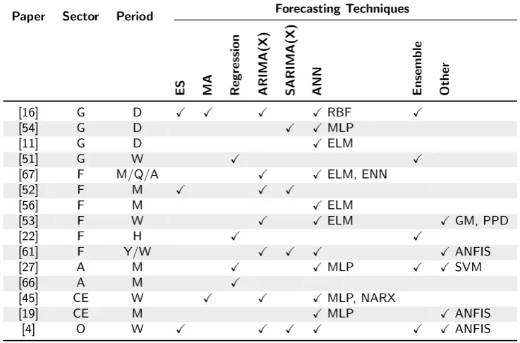
“dairy”) and perishability are provided. For this study, only perishable products will be considered, which leaves a dataset with 986 perishable items. The large size of this dataset makes it a good basis for a robust comparison of different demand fore-casting techniques. Table 3.1 gives an overview of the different perishable product categories that are present in the dataset and what percentage of items falls in each of those categories.
3.3.2
External Factors Considered
Figure 3.1 gives an overview of the external factors that are taken into account in this study, which fall in the weather, events, economic and promotions categories. Daily Ecuadorian weather data was obtained from DarkSky2. The weather data includes minimum and maximum temperature, cloud cover, humidity, dew point, visibility and wind speeds for the cities where the 54 Favorita stores are located. Data for the other external factor categories was already included in or derived from the Favorita dataset. The events data that is used contains days of the week and national Ecuadorian holidays (regional holidays were excluded). Three types of holidays were distinguished: holidays, events and additional days. Additional days are the days around holidays or events, such as the days before Christmas. The promotions data that is used contains whether a product was on promotion (true or false). The economic data that is used the daily oil prices in Ecuador.
The options for external factor feature selection were evaluated as well, although not automatically for each individual item during the evaluation since this would
2DarkSky API:
CHAPTER 3. RESEARCH METHOD 32
consume too much time. A manual evaluation was performed on a small subset of items where the K (= 5, 10, 15, 20, all) best features were selected based on the mutual information scores. This indicated that using all features resulted in the best performance.
When comparing figure 3.1 with figure 2.3 which provided an overview of all external factor categories that could be used for demand forecasting, it can be seen that some external factor categories were not considered during this study. External factors from the product, competitors, social media and search trends categories were not considered, since such data was unfortunately not available. For example, no detailed product information and no price information was available because Favorita anonymized the publicly available dataset. To find relevant social media messages or search trends, at least brand and preferably product names would have to be available.
3.3.3
Data Preprocessing
No special data preprocessing was necessary for NAIVE, MA and ES. Since ARIMA assumes that the data is stationary and that it has a zero mean, some pre-processing was required to make sure these assumptions are met. The raw time series data was demeaned to make sure it had a zero mean. The augmented dickey-fuller (ADF) test was performed to check whether the time series is stationary before applying the ARIMA model. For the LINREG, ADA, SVR, MLP and LSTM models more pre-processing was required and in particular the data is scaled so all features have the same scale and have values between 0 and 1.
4
Performance Comparison
Results
This chapter covers the results from the performance comparison of DF techniques. Section 4.1 discusses results for the one-step ahead forecasting scenarios, section 4.2 for the multi-step ahead forecasting scenarios and section 4.3 covers the results on the influence of external factors.
For each scenario, a table is provided with for each DF technique the average, minimum and maximum RelRMSE score. The average RelRMSE score can be seen as a measure of each technique’s performance consistency, since it reflects how well it performs on average across all items. When a retailer wants to use a single forecasting technique for all its items, he most likely wants to choose the DF technique that performs best on average (lowest average RelRMSE). The last row in each table, with ‘BEST’, reports the RelRMSE score when the best-performing DF technique was chosen for each individual item. The last column in the table reports the %best, which is the percentage of items for which each DF technique was the best-performing one. When the retailer wants to use an algorithm that automatically selects the best DF technique for each item, the best% score reflects how important it is to include each DF technique in the set of techniques the forecasting algorithm can choose from.
Wilcoxon signed-rank tests were conducted for all pairs of DF techniques in each scenario to test whether the distributions of their RelRMSE scores were significantly different. More details about this test and the significance test results can be found in appendix B.
4.1
Results for One-Step Ahead Scenarios
This section first describes the results for each individual one-step ahead scenario and then discusses the results in a cross-scenario comparison.
OWC Scenario results
Table 4.1 contains the RelRMSE scores for the OWC forecasting scenario. ARIMA performed best for the largest amount of items (27.6%), followed closely by LINREG (24.0%) and ADA (18.9%). When looking at performance consistency, it can be