First observation of the charmless decay B+ > K+π0π0 and study of the Dalitz plot structure

(1)

University of Warwick institutional repository: http://go.warwick.ac.uk/wrap

A Thesis Submitted for the Degree of PhD at the University of Warwick

http://go.warwick.ac.uk/wrap/49168

This thesis is made available online and is protected by original copyright. Please scroll down to view the document itself.

(2)

First observation of the

charmless decay

B

+

→

K

+

π

0 π

0 and study of the Dalitz plot structure

Eugenia Maria Teresa Irene Puccio

Thesis

Submitted to the University of Warwick for the degree of

Doctor of Philosophy

Department of Physics

University of Warwick

(3)

(4)

List of Figures

1.1 The unitarity triangle with three mixing angles and sides as a function

of the elements in the CKM matrix. . . 6

1.2 Constraints in the (¯ρ,η¯) plane including recent measurements of α

and γ in the global CKM fit. The red hashed region of the global

combination corresponds to 68% confidence level (CL) [19]. . . 7

1.3 Box diagram forB0_B0 _{mixing via the exchange of two} _W _{bosons. . .} ₉

1.4 Feynman diagrams forB _→Kπ: (a) tree and (b) penguin. . . 13

1.5 Feynman diagrams for the decay processes in B+ _→_K∗+_π0 _{. . . 17}

1.6 Relation between the four K∗_π _{decays and the six} _Kππ _{decays. . . . 18}

1.7 Illustration of a sample Dalitz plot (left) and square Dalitz plot

(right) obtained from toy MC events and showing B+ _→_K+_π0_π0

non resonant (black) and the resonances B+ _→_K∗₍₈₉₂₎+_π0 _(red),

B+_→_K∗+

2 (1430)π0(cyan),B+ →f0(980)K+(green),B+ →f2(1270)K+

(magenta) andB+ _→_χ

c0K+ (blue). . . 21

2.1 A schematic of the PEP-II rings and the collision region. The blue

(11)

2.2 Schematic of the PEP-II interaction region. The pink areas around

the interaction point represent the dipole magnets used to bring the

beams together and the regions with a Q label indicate the positions of

the various quadrupole magnets. (Graphic source: SLAC Accelerator

Systems Division via Ref. [44]) . . . 24

2.3 Luminosity distribution over the experiment running period [47]. . . . 25

2.4 Longitudinal section and front end view of the BaBar detector. [48] . 27

2.5 The SVT (a) fully assembled with visible outer layers and carbon

fibre frame and (b) schematic view of the transverse section with the

various layers around the beam pipe [48]. . . 28

2.6 Longitudinal cross section of the DCH with the principal dimensions

in mm and offset with respect to interaction point (IP) [48]. . . 30

2.7 Measurement of the average dE/dx as a function of track momenta

from the DCH. The curves superimposed to the data show the

Bethe-Bloch predictions for energy loss of a sample of particles of different

masses [48]. . . 31

2.8 Schematics of the DIRC fused silica radiator bar [48]. . . 32

2.9 Expected K/π separation as a function of track momentum [48]. . . . 33

2.10 A longitudinal cross-section of the EMC indicating the arrangements

of the 56 crystal rings. All dimensions are given in mm [48]. . . 34

2.11 Overview of the IFR showing barrel sectors and forward and backward

end doors. The shape and dimensions of the RPC modules are also

shown. [48] . . . 36

(12)

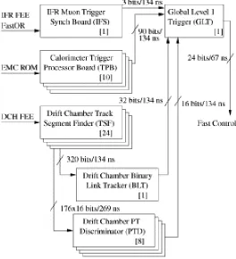
2.13 Simplified L1 trigger schematic. Indicated in the figure are the

num-ber of components and the transmission rates between them in terms

of signal bits. [48] . . . 38

3.1 Layout of a Multilayer Perceptron with one hidden layer [56]. . . 47

3.2 An example ∆E sPlot (data points) for signal (left) and background

(right) obtained from a maximum likelihood fit to the sample mES

distribution only. Overlayed is the distribution generated from the

Gaussian and linear PDFs (blue line). . . 52

4.1 Distributions for signal MC (blue line) and offpeak data (red line)

of the ratio of Legendre polynomials, L2

L0. Both distributions were

normalised to unity. . . 59

4.2 Absolute value of the cosine of theB direction on the left and the B

thrust to the right with respect to the beam axis for signal MC (blue

line) and offpeak data (red line). Both distributions were normalised

to unity. . . 60

4.3 Absolute value of the output of the flavour tagging NN for signal MC

(blue line) and offpeak data (red line) . . . 61

4.4 Comparison of the performance of three MVAs using the same

vari-ables. The MLP Neural Network gives the best performance for this

mode. . . 61

4.5 Correlation matrices between the five event shape variables for signal

MC and offpeak data. . . 62

4.6 Neural Network distribution for signal Monte Carlo and offpeak data.

The green arrow indicates the position of the selection applied on the

(13)

4.7 π0_π0 _{invariant mass distribution in}_B+ _→_K0 SK

+_{, K}0 S →π

0_π0 _Monte

Carlo before the veto is applied. The arrows indicate the vetoed region. 64

4.8 Variation of signal efficiency over the conventional Dalitz plot (left)

and square Dalitz plot (right). . . 66

4.9 Difference between generated and reconstructed momenta divided

by reconstructed momentum error plotted against reconstructed

mo-menta for lowest momentumπ0 _{candidate (left), highest momentum}

π0 _{candidate (centre), kaon candidate (right). . . 67}

4.10 mES and ∆E distributions for different ranges ofxi, wherexi is ppull

for all three final state particles. . . 69

4.11 mES (left) and ∆E (right) distributions for TM (red histogram) and

SCF (blue histogram) events based upon a definition of SCF from

ppull >5.0. Both TM and SCF histograms have been normalised. . . 70

4.12 Fraction of self cross feed events as a function of Dalitz plot position

in conventional (left) and square (right) Dalitz plot form. . . 70

5.1 Variation of the signal mES, ∆E and NNout distributions over the

Dalitz plot in terms of the mean and rms of the distributions. These

Dalitz plots were constructed from nonresonant signal MC events that

lie in the signal region ofmES and ∆E (see Section 5.1.2). The events

were selected as described in Chapter 4 except that the K0

SK

+ _veto

was not applied. . . 74

5.2 mES and ∆E distributions for signal MC (black line), continuum

background (red line), generic B+_B− _{MC (green line) and generic}

B0_B0 _{MC (blue histogram). The black dashed arrows indicate the}

(14)

5.3 Signal PDF distributions (red line) overlaid on nonresonant MC (black

data points) for TM mES (left) and NNout histogram (right). . . 79

5.4 Control channel, B+ _→ _D0_ρ+ _→ ₍_K+_π−_π0_{) (}_π+_π0_{), PDF}

distribu-tions (red line) overlaid on MC (black data points) formES (left) and

NNout histogram (right). . . 80

5.5 (Left)mES and (right) NNout projection distributions from the fit to

the control channelB+_→_D0_ρ+ _→₍_K+_π−_π0_{) (}_π+_π0_{). Black markers}

are the data points with fit overlaid (blue line), green dashed lines

are theBB background, red dotted lines the continuum background

and black dashed lines the signal. . . 81

5.6 Signal (left) and continuum (right) sPlot distributions for mES

ob-tained from a fit to the control channelB+ _→_D0_ρ+_→₍_K+_π−_π0_{) (}_π+_π0_).

Black dots show thesPlotdistributions and the red lines show the fit

results. . . 82

5.7 Signal PDF distributions (red line) overlaid on nonresonant MC (black

data points) for SCF signal mES (left) and NNout (right). . . 84

5.8 qqPDF distributions (red line) overlaid on: offpeak data formES(left)

and USB and GSB onpeak data withBB background subtracted for

NNout (right). . . 85

5.9 Distributions of mES (left), NNout (centre) and ∆E (right) for: (a)

category 1 BB backgrounds, (b) category 2 BB backgrounds, (c)

category 3 BB backgrounds, (d) category 4 BB backgrounds. . . 88

5.10 Gaussian fits to the distributions of fitted SCF fractions and signal

yields. The toy experiments are generated from: nonresonant MC –

expected SCF fraction 5.3 % (left);K∗₍₈₉₂₎+_π0 _{MC – expected SCF}

(15)

5.11 Signal Dalitz plot distributions calculated from the signal MC (right)

and from thesWeights (left) for the nonresonant mode. The Dalitz

plot distribution to the left is obtained by running a toy experiment

of 100 times the number of expected signal events. . . 95

5.12 (Top)mK+_π0

min distribution in theK

∗+_{(892) region from} _K∗₍₈₉₂₎+_π0

(left) and nonresonant (right) MC; (Middle)mπ0_π0 distribution in the

f0(980) region, from f0(980)K+ (left) and nonresonant (right) MC;

(Bottom)mπ0_π0 distribution in theχ_c₀ region, fromχ_c₀K+ (left) and

nonresonant (right) MC. The arrows in the left plots indicate the

selection requirements of signal (red) and sidebands (green) used for

the sideband subtraction. The blue line represents the fit to the MC

data. . . 100

6.1 Pull and fitted uncertainties distributions for B+_→_K+_π0_π0

nonres-onant, B+ _→_K∗₍₈₉₂₎+_π0 _and _B+_→_f

0(980)K+ obtained from 500

pure toy experiments. . . 104

6.2 Projections ofmES (left) and NNout (right) for the fit to: (a) offpeak

data and (b) blind fit to onpeak. The data points (black) show the

sPlot distribution for the continuum background and the line

(ma-genta) is the background PDF generated from the fit. . . 108

6.3 Projection distributions for mES (left) and NNout (right) after

im-plementing the additional requirements on the other fit variable to

enhance the signal visibility. Points with error bars show the data,

the solid (blue) line represent the total fit result, the dashed (green)

curves show the total background contribution and the dotted (red)

curve is theqq component of the background. The dash-dotted curve

(16)

6.4 Signal sPlot distributions (black data points) with PDF (red line)

overlaid, where appropriate, for mES (top left), NNout (top right),

∆E (bottom center). . . 110

6.5 Negative log likelihood distribution versus signal yield. . . 111

6.6 Signal Dalitz plot distribution, obtained usingsWeights, for

conven-tional (left) and square (right) Dalitz plots for uncorrected (top) and

corrected for efficiency using the signal MC efficiency from Figure 4.8

(bottom). . . 112

6.7 Signal sPlot distributions for mKπ0

min (a) over all mass range, (b)

zoomed into mass range 0.5< mKπ0

min <2.0GeV /c

2_{. . . 114}

6.8 SignalsPlotdistributions formπ0_π0 (a) over all mass range, (b) zoomed

into mass range 0.5 < mπ0_π0 < 2.0 GeV /c2, (c) zoomed into mass

range 3.0< mπ0_π0 <4.0GeV /c2. . . 115

6.9 Typical sPlot distributions obtained from one experiment in each

cocktail mixtures for: (left to right)mK+_π0

mindistribution in theK

∗+₍₈₉₂₎

region, mπ0_π0 distribution in the f₀(980) region; and m_π0_π0

distribu-tion in the χc0 region. χc0, K∗(892)+ and f0(980) are missing from

one cocktail in this order. Red (green) arrows indicate the signal

(sidebands) region. . . 117

6.10 Distribution of branching fractions from each cocktail for: (from left

to right)K∗₍₈₉₂₎+_π0_,_f

0(980)K+ andχc0K+. The distributions were

(17)

6.11 Mass region distributions for K∗₍₈₉₂₎+ _{(top left),} _f

0(980) (top right)

and χc0 (bottom) from data with fit result overlaid. The black data

point show the sPlot data, the blue continuous line is the overall

fit and the red dashed the nonresonant contribution. The red and

green arrows indicate the signal and sideband regions used in the

subtraction method. . . 121

7.1 Pull distributions for the signal asymmetry with error distributions on

the right obtained from generated samples with asymmetries ₋40%

(top row), 0% (middle row) and 40% (bottom row). . . 124

7.2 Projection plots onmESand NNout from the fit to data for the positive

charged decay,qB = 1 (left plot) and negative charged decay,qB=−1

(right plot). Points with error bars show the data, the solid (blue)

line represent the total fit result, the dashed (green) curves show the

total background contribution and the dotted (red) curve is the qq

component of the background. The dash-dotted curve represents the

signal contribution. . . 126

7.3 Result of fit in the mass region of K∗₍₈₉₂₎+ _(top), _f

0(980) (middle)

andχc0(bottom) forB+decay (left) andB−decay (right). The black

points show the sPlot data, the blue continuous line is the overall fit

and the red dashed line the NR contribution. Red (green) arrows

indicate the signal (sidebands) region. . . 127

8.1 Linear correlations coefficients obtained from the fit to the mES

dis-tribution of theB+ _→_D0_ρ+_→₍_K+_π−_π0_{) (}_π+_π0_{) MC control sample. 131}

8.2 Ratio of the NNout sPlot distribution and the MC based PDF for the

(18)

8.3 Distributions of SCF events in mES and NNout for nonresonant and

resonant decay modes. Refer to Table 3.1 to match the MC number

to a specific decay. . . 133

8.4 Projection plots onmES and NNout from the fit to the control sample

for the positive charged decay (left plot) and negative charged decay

(right plot). Points with error bars show the data, the solid (blue)

line represent the total fit result, the dashed (green) curves show the

total background contribution and the dotted (red) curve is the qq

component of the background. The dash-dotted curve represents the

signal contribution. . . 139

A.1 Dalitz plot dependences of the mean and width of the distributions

for ∆E, |_σ∆t|

∆t, the NNout, as a consequence of the dependence in

|∆t_| σ∆t,

and finally ∆_σ E

∆E. . . 153

A.2 Migration of (a) TM and (b) SCF events within the Dalitz plot,

plot-ted at their MC truth coordinates. Note the different scales on the

z-axes. . . 155

A.3 Signal yield distributions from embedded signal MC toy with 500

experiments. The red arrow indicated the expected yield with a loose

∆E signal region of 673 events. Biases range from 40 events to as

high as 171 for resonances decaying to π0_π0_{. . . 156}

B.1 Single ratio momentum distributions of (left) charged pions in the

zero bump sample and (right) neutral pions in the one and two bumps

samples. The red line is the distribution obtained from MC and black

line data. The blue data points with blue axis to the right show the

(19)

B.2 Double ratio as a function of π0 _{momentum using additional}

require-ments from the Pi0AllLoose list. The black data points show the

ratio of the π0 _{momentum of 1 and 2 bump events to pion}

momen-tum for events with no bumps. The green line indicates the first order

polynomial fit to the double ratio. . . 164

B.3 Double ratio as a function of π0 _{momentum using additional}

require-ments from the Pi0AllLoose list. The black data points show the

nominal double ratio distribution with statistical errors and the red

extended error bars the additional uncertainty from the

systemat-ics. The green line is the linear fit to the double ratio that includes

(20)

List of Tables

1.1 Experimental results [33] and theoretical fit predictions for the

branch-ing fractions and CP asymmetries for all B _→ Kπ and ∆ACP,

ob-tained using the diagrammatic approach. C(K0

Sπ

0_{) and}_S₍_K0

Sπ

0_{) are}

the parameters of the time-dependent amplitude in Eq. 1.20. The fit

prediction of ∆ACP is obtained by removing both ACP(K+π0) and

ACP(K+π−) from the fit [1]. . . 14

1.2 Branching ratios (in units 10−6_{) and direct} _CP _{asymmetries (in units}

10−2_{) obtained from the QCDF method [35]. . . 15}

1.3 Amplitudes, branching fractions and asymmetries for B _→ Kπ and

B _→K∗_π _{modes, including}_B0 _→_π+_π−_and _B0 _→_ρ+_π−_{. Branching}

fraction and ACP averages are taken from Ref. [33]. . . 18

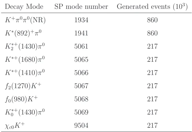
3.1 List of nonresonant and resonant MC modes. The “SP” followed by

the mode number is a unique identifier for each signal decay. . . 43

3.2 The “R24a3-v03” dataset . . . 44

4.1 PID selector performance for B+ _→_K+_π0_π0_{. . . 58}

4.2 Selection cut summary and efficiencies for the NR modeK+_π0_π0 _and

(21)

4.3 Summary of veto efficiency, average efficiency and SCF fraction for

all nonresonant and resonant signal modes. . . 71

5.1 An overview of the fitting model giving a description of the PDFs

including if the parameters are fixed or floated in the fit. . . 73

5.2 Correlations with Dalitz plot coordinates ofmES, ∆E and NNout

dis-tributions. . . 75

5.3 Optimisation of the ∆E cut. For each set of cut values, the total

sig-nal efficiency, expected number of background events, the Punzi FOM

and the ∆E cut efficiency based on nonresonant MC. The coloured

row indicates the signal selection used. . . 76

5.4 Signal mES PDF parameters obtained from fit to control sample in

MC and data, together with the obtained data/MC calibration

fac-tors. . . 83

5.5 The uncorrected values of the parameters for the TM signal mES

Cruijff, obtained from a fit toB+_→_K+_π0_π0 _{nonresonant MC with}

errors, together with the values calibrated using the data/MC

correc-tion factors and errors obtained from the control sample Table 5.4. . 83

5.6 Parameters of the signal SCFmES PDF (a 3rd order Chebychev

poly-nomial). Values and their uncertainties are obtained from a fit to the

nonresonant MC distributions. All of these parameters are fixed in

the fit to data. . . 84

5.7 Parameters for the qq mES PDF. The initial value given is obtained

from the fit to offpeak data. . . 85

5.8 Initial values of the parameters for the qq NNout PDF obtained from

a fit to the sideband regions (USB and GSB) in onpeak with BB

(22)

5.9 Expected numbers of events used in the generation process in each

signal and background category and their status in the fit.

Uncer-tainties on the measured values are given for the fixed yields. . . 91

5.10 Table of branching fractions and CP asymmetry (if known) for each

B background mode along with the expected number of events in the

signal region. The “DP” next to the mode description indicates that

the Dalitz plot model is used and therefore MC includes nonresonant

and resonant contributions. The values listed are found using the

world averages taken from HFAG [33] and PDG [38]. A decay with†

indicates that the full or part of the branching fraction was estimated

using isospin relations. . . 92

5.11 Table of values of fSCF, calculated using sWeights, and signal yields

after each iteration, up to convergence, of the fit to single toy

experi-ments generated using MC for each nonresonant (NR),K∗₍₈₉₂₎+_π0_,

K∗+

2 (1430)π0, K∗+(1410)π0 and f2(1270)K+. . . 93

5.12 Selection requirements used to isolate resonances in the relevant MC

samples. Units of GeV/c2 _{have been suppressed. . . 97}

5.13 Parameters obtained from an unbinned fit to the signal MC mass

distributions. These are all fixed in the fit to the mass sPlot. . . 98

5.14 Fit parameters obtained from the nonresonant MC in the resonance

mass region. These parameters are allowed to float in the fit to the

mass sPlot. . . 99

6.1 Mean and width of the pull distributions together with the mean of

the signal yield uncertainties and their errors obtained from pure toy

experiments forB+_→_K+_π0_π0 _nonresonant, _B+ _→_K∗₍₈₉₂₎+_π0 _and

B+_→_f

(23)

6.2 List of signal yields and biases for the embedded toy experiments

using nonresonant and all resonant signal MC. . . 105

6.3 Results for the signal yield in one toy experiment embedding

sig-nal and BB backgrounds with 3_× the statistics for nonresonant,

K∗₍₈₉₂₎+ _and _f

0(980). . . 106

6.4 Yield results for the fit to offpeak data allowing for a signal component

including the errors. . . 107

6.5 Results at each iteration for fSCF and signal yield of the fit to data

up to convergence. . . 109

6.6 Number of events for each signal MC used to reproduce the total yield

and preserve the overall SCF fraction. This mixture also reproduces

the broad features of the Dalitz plot. . . 113

6.7 Composition of the cocktail Monte Carlos. Events are drawn from

large samples – the numbers quoted are the average numbers of events

from each SP mode in each cocktail experiment. The corresponding

branching fractions (in units of 10−6_{) for the Q2B decays are also}

given. . . 116

6.8 Efficiencies of mass cut selections of the signal region and (signal+sidebands)

regions obtained from the MC samples of each resonance. . . 118

6.9 Validation of the method to determine quasi-two-body branching

frac-tions. The values given are the measured branching fractions (in units

of 10−6_{) for each cocktail and are taken from Gaussian fits to the BF}

distributions in Figure 6.10. The uncertainty is the width of the

Gaussian, which we use as an estimate of the statistical uncertainty

of the result of one experiment. . . 118

(24)

6.11 Mean branching fractions and bias obtained for each resonance from

a cocktail reflecting the number of events observed in data. These

results were obtained using the subtraction method. . . 120

7.1 List of values for theACP used in toy MC generation and their status

in the fit. . . 123

7.2 List of signal asymmetries and biases on the asymmetry obtained

from fits. . . 125

7.3 B+ _and _B− _{yields for each resonance obtained using the background}

subtraction method. . . 128

8.1 Results of the fits made by varying theBB background yields within

their uncertainties. This table lists the differences between signal

yields obtained in these fits and the nominal value. . . 134

8.2 Summary of systematic uncertainties associated to the fit model for

the inclusive branching fraction measurement ofB+_→_K+_π0_π0_{. . . . 135}

8.3 Summary of systematic uncertainties due to PID and selection

effi-ciencies in the inclusive branching fraction measurement ofB+ _→_K+_π0_π0_.138

8.4 Variation in the fitted signalACP with varyingBBbackground

asym-metries. . . 140

8.5 Summary of systematic uncertainties for asymmetry measurement. . 141

8.6 Variations in the nominal result using reduced sidebands. . . 142

8.7 Variation of the signal cut efficiency in the MC with fSCF. . . 143

8.8 Summary of systematic uncertainties on the branching fraction

(25)

9.1 Comparison of our results to previous measurements [33, 38]. The

world averages of the branching fraction andCP asymmetry ofB+ _→_K∗₍₈₉₂₎+_π0

come from a sole prior measurement byBA_BAR_{[3] and are superceded}

by our results. Note that the decayB+ _→_χ

c0K+andACP ofB+→f0(980)K+

have been studied in theK+_π−_π+ _{final state, giving more precise}

re-sults. . . 147

B.1 Branching fractions forτ leptons to final states containing one charged

track with or without additional neutral particles (γ, π0 _or _η_{), from}

(26)

Acknowledgements

I would like to thank the Particle Physics Group at the University of Warwick for

giving me the opportunity to work with them; it was a pleasure to be a part of

this group and learn from such amazing people. In particular I would like to thank

Dr. Tim Gershon for all his support, advice and encouragement in what turned

out to be quite a tricky and challenging analysis. I also would like to thank STFC

for providing the funding for my Ph.D and my long term attachment in California,

which allowed me to become more involved within the Collaboration.

A particular thanks to the amazing people I met along the way both at Warwick

and in California who have contributed to make these four years so enjoyable. To

Andy Bennieston, Nicola McConkey, Nikola Chmel, Leigh and Mark Whitehead for

always being there for me and keeping me company in the essential coffee breaks.

To everyone at SLAC: Mark Tibbetts, Sudan Paramesvaran, Michael Sigamani,

Jen Watson and in particular Kim Alwyn, Graham Jackson, Jasmine Hasi, Manuel

Franco and Aidan Randle-Conde for making my life experience in America so fun

and every Collaboration Meeting interesting! A very special thanks to Aidan and

Jelena Ilic for their friendship and support in overcoming the hardest and most

difficult time of my life. I would not have been able to finish this work without you!

To Jean Sutherland and George Lafferty for their support while on LTA and for

making those dinner parties in California so special.

A very special thanks to Tom Latham who taught me so much, not only about

Particle Physics and programming, but also about life. You have been there for me

(27)

partner in life.

Finally to my family, to whom I dedicate this thesis, because without your love and

faith in me this thesis would have never happened. In particular to my mother who

gave me all her support and encouragement even in the final moments of her life

(28)

Declaration

I declare that the work in this thesis was carried out in accordance with the

Regu-lations of the University of Warwick. No part of this thesis has been submitted for

any other academic award at this or any other university.

The data used in this analysis was recorded by the BABAR detector run by the

BABAR Collaboration. The author contributed to the running of the detector by

taking general shifts, being Run Quality Manager for the reprocessing of the final

dataset, used in this analysis, and performing the neutral pion efficiency study in

Appendix B. The event reconstruction uses code developed by the Collaboration,

with packages for 3-bodyB meson decay reconstruction and final selection (QnBUser

and CharmlessFitter) written by Dr. Fergus Wilson and Dr. Thomas Latham

respectively. The software used for the likelihood fit (Laura++) was first developed

by Prof. Paul Harrison, Dr. John Back and Dr. Thomas Latham, further extended by

the author to incorporate the PDF needed for misreconstructed signal modelling.

The π0 _{efficiency study code in Appendix B was mostly written by Dr. Thomas}

Latham with significant contributions from the author and Dr. Tim Gershon. The

likelihood scan (Figure 6.5) used to determine the statistical signal significance and

the final calculation of the π0 _{efficiency corrections (part of Section 6.3.3) was done}

by Dr. Thomas Latham. The remainder of the work described in this document

(Chapters 4–8 and all Appendices) was carried out solely by the author with support

from Dr. Tim Gershon, Dr. Thomas Latham and the Charmless 3-body Analysis

Working Group from BABAR. All views expressed are those of the author.

(29)

Abstract

Results for the first measurement of the inclusive branching and CP asymmetry of

the charmless 3-body decayB+ _→_K+_π0_π0 _{are presented. The analysis uses a data}

sample with an integrated luminosity of 429.0 fb−1, recorded by theBA_BAR _detector

at the PEP-II asymmetricBFactory. This sample corresponds to 470.9_±2.8 million

BBpairs. Measurements of the branching fractions (_B) andCP asymmetries (ACP)

of some of the intermediate resonances in theK+_π0_π0_{Dalitz plot are also presented.}

The results are summarised here:

⋄ B(B+ _→_K+_π0_π0_{) = (16}_.₂_±₁_.₂_±₁_.₄₎_×₁₀−6

⋄ B(B+ _→_K∗₍₈₉₂₎+_π0_;_K∗0₍₈₉₂₎_→_K+_π0_{) = (2}_.₇₂_±₀_.₅₀_±₀_.₃₄₎_×₁₀−6

⋄ B(B+ _→_f

0(980)K+;f0(980)→π0π0) = (2.77±0.56±0.43)×10−6

⋄ B(B+ _→_χ

c0K+;χc0 →π0π0) = (0.51±0.22±0.09)

⋄ ACP(B+ →K+π0π0) = (−6±6±4) %

⋄ ACP(B+ →K∗(892)+π0) = (−4±26±4) %

⋄ ACP(B+ →f0(980)K+) = (17±18±4) %

(30)

Introduction

This thesis presents the first study of the charmless 3-body decay, B+ _→_K+_π0_π0_.

It includes the inclusive measurement of the branching fraction andCP asymmetry.

Additionally a study is performed on the Dalitz plot to obtain the branching fractions

and CP asymmetries of the following intermediate quasi-two-body decays: B+ _→

K∗₍₈₉₂₎+₍_→ _K+_π0₎_π0_, _B+ _→ _f

0(980)(→ π0π0)K+ and B+ → χc0(→ π0π0)K+.

The ACP measurement of B+ →K∗(892)+π0 is particularly interesting in the light

of new theoretical approaches to study the “Kπ” puzzle in theK∗_π _{system [1,2]. A}

previous measurement of the quasi-two-body decay ofB+ _→_K∗+_π0_{was published in}

Physics Review Letters by theBA_BAR_{Collaboration. This analysis used 232 million}

BB pairs and obtained a branching fraction of _B(B+ _→_K∗₍₈₉₂₎+_π0_{) = [6}_.₉ _±

2.0(stat.)_±1.3(sys.)]_×10−6_{, with a statistical significance of 3}_._{6 standard deviations,}

and an asymmetry ofACP(B+ →K∗(892)+π0) = 0.04±0.29(stat.)±0.05(sys.) [3].

The large statistical error associated to the asymmetry measurement makes it hard

to extract conclusive results and a more precise measurement is needed. This thesis

makes use of the fullBA_BAR_{dataset of 470}_._{9 million}_BB_{events collected at the}_Υ₍₄_S₎

resonance, more than double the dataset available in the previous measurement.

Since the asymmetries forB+_→_f

0(980)K+andB+→χc0K+are already measured

in theK+_π+_π−_{final state [4,5], these results serve as a cross-check of the procedure.}

The branching fractions of the decays B+_→_K∗₍₈₉₂₎+_π0 _and _B+ _→_χ

c0K+ serve

mainly as a cross-check from previous world average measurements, correcting for

K∗₍₈₉₂₎+ _→ _K+_π0 _and _χ

c0 → π0π0 assuming isospin conservation. However it is

(31)

2

this mode the ratio of product branching fractions is quoted instead:

B(B+ _→_f

0(980)K+)× B(f0(980)→π0π0)

B(B+_→_f

0(980)K+)× B(f0(980)→π+π−)

= B(f0(980)→π

0_π0₎

B(f0(980)→π+π−)

(1)

The prediction from isospin symmetry is that the ratio of these two decays should

(32)

1

Theoretical Motivations

Until 1964, the weak interaction was known to violate both charge conjugation

and parity transformation individually. However in that year evidence of violation

of the combination of these two transformations, known as CP, was found in the

decay channel KL → π+π− at Brookhaven National Laboratory [11]. CP violation

is one of the three Sakharov conditions required to explain the matter-antimatter

asymmetry in the Universe [12]. The primary goal of the BABAR experiment is

the study of CP asymmetries and the measurement of CP violation parameters in

the B meson system. This chapter introduces the concept of CP asymmetry and

the Standard Model formalism. It also introduces the primary motivations for this

measurement,i.e. the study of the equivalent of the so called “Kπ puzzle” in K∗_π

(33)

1.1. Flavour mixing and the CKM formalism 4

1.1 Flavour mixing and the CKM formalism

This chapter gives a brief overview of the theory behind the CKM matrix and its

formulation in the Standard Model. For a more detailed derivation of the CKM

formalism refer to Refs. [13–16]. In the Standard Model, all matter is made up of

quarks and leptons each of which comes in six different types or “flavours”. Quark

flavours change under the charged current weak interaction. These flavour changing

quark transitions are described by the following Lagrangian:

L(CC)₌₋_√g

2(J

µ

(CC)Wµ(+)+J

†µ (CC)W(

−)

µ ) (1.1)

whereW±

µ represents the charged vector boson field,g is the weak coupling constant.

The operatorJ₍µ_CC₎ is the weak charged quark current operator and takes the form:

J₍µ_CC₎ = ¯uLγµdL (1.2)

where (uL, dL) is the notation for the left-handed SU(2) quark doublet and γµ the

Dirac matrices. To represent fully the mass eigenstates that propagate through

space and time, it is useful to transform the Lagrangian to the mass basis. Denoting

the unitary basis transformation _S, the quark flavour basis is rotated to states of

definite mass,um

L and dmL, by writing:

um_L =_S_LuuL dmL =SLddL (1.3)

Using the transformation in the expression for the charged weak currents coupling

uL todL, becomes:

J₍µ_CC₎ = ¯um_Lγµ(_S_Lu_S_Ld†)dm_L (1.4)

This expression shows the origin of the unitary matrix V _{≡ S}u

LS d†

L also known as

the CKM matrix, which was named after the theorists Cabibbo, Kobayashi and

Maskawa [17, 18]. Each up-type quark couples to a mixture of down-type quarks so

that the CKM matrix defines the rotation from the down-type quark states produced

(34)

“seen” by the weak interaction (d′_,_s′ _and _b′_):



 

d′

s′

b′ 

  =



 

Vud Vus Vub Vcd Vcs Vcb Vtd Vts Vtb



 



 

d s b





 (1.5)

The origin of the CKM matrix is related to the fermion masses via the Yukawa

interaction. The Lagrangian of the Yukawa interaction takes the form:

LY =−Yijuq¯LiφuRj−Yijdq¯Liǫφ∗dRj (1.6)

where Yu,d _{are 3}_×_{3 complex matrices,} _ǫ _{is a 2}_×_{2 antisymmetric tensor,} _φ _{is the}

Higgs field and indices run over the flavour generations. Whenφ acquires a vacuum

expectation value, the Yukawa interaction yields non-diagonal mass matrices for

the quarks. To determine the quark masses, Yukawa terms have to be diagonalised

by different transformations for left-handed up and down quarks. As a result the

charged current interactions couple to um

L and dmL states shown in Eq. 1.3 with

couplings given by the elements of the CKM matrix.

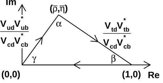
1.1.1 The unitarity triangle

The CKM matrix has four independent parameters, which can be thought of as three

mixing angles between the three pairs of quark generations and a complex phase.

The unitarity requirement of the CKM matrix places the following constraint on its

elements:

VudVub∗ +VcdVcb∗ +VtdVtb∗ = 0 (1.7)

This is only one of six orthogonality constraints and each can be represented as a

triangle in the complex plane. Eq. 1.7 is known by theB Factories as “the unitarity

triangle” and is shown in Figure 1.1. Each angle of the triangle is given by ratios of

(35)

[image:35.595.202.467.134.269.2]

Re

Im

cb *

V

cd

V

ub *

V

ud

V

cb *

V

cd

V

tb *

V

td

V

γ

α

β

)

η

,

ρ

(

(0,0)

(1,0)

Figure 1.1: The unitarity triangle with three mixing angles and sides as a

function of the elements in the CKM matrix.

α=₋arg VtdV

∗

tb VudVub∗

!

(1.8)

β =₋arg VcdV

∗

cb VtdVtb∗

!

(1.9)

γ =₋arg VudV

∗

ub VcdVcb∗

!

(1.10)

and can be experimentally determined via specific decay modes. A few examples

include the time dependent analysis ofB0 _→_{J/ψ K}0

S, also known as the golden mode

for measuring β, and Cabibbo suppressed modes like B _→ DD. Measurements of

the angles and sides have to be made through as many independent decay modes

as possible to overconstrain the triangle and to be able to probe for contributions

from physics beyond the Standard Model. All measurements are then combined into

a fit, an example of which is shown in Figure 1.2. The area of the triangle gives

a convention independent measure of the amount of CP violation in the Standard

(36)

γ

γ α

α

d

m

∆

K

ε

K

ε

s

m

∆

&

d

m

∆

ub

V

β

sin 2

(excl. at CL > 0.95) < 0

β

sol. w/ cos 2

excluded at CL > 0.95

α

β γ

ρ

-1.0 -0.5 0.0 0.5 1.0 1.5 2.0

η

-1.5 -1.0 -0.5 0.0 0.5 1.0 1.5

excluded area has CL > 0.95

ICHEP 10

CKM

[image:36.595.165.484.258.573.2]

f i t t e r

Figure 1.2: Constraints in the (¯ρ,η¯) plane including recent measurements of

α andγ in the global CKM fit. The red hashed region of the global combination

(37)

1.2. CP violation 8

1.2 CP

violation

This section gives a brief overview of the different types ofCP violation observed in

meson decays. For a more detailed description refer to Refs. [20, 21]. In quantum

theory a transformation maps a state to another through a unitary operator U

where the unitarity condition is required to maintain normalisation. This can be

generalised by:

|Ψ_{i → |}Ψ′

i=U_|Ψ_i (1.11)

The symmetry properties of a physical system arise by the invariance of the measured

quantities when performing a transformation. A symmetry violation occurs when a

symmetry, well-established in a class of physical processes, is broken under certain

circumstances. The discrete transfomations of interest here in particle physics are

listed below.

⋄ Charge conjugation: this is the process associated with the exchange of

particles and antiparticles under the transformation of all charges into their

opposite sign by the unitary operator, C. Charge conjugation symmetry

re-quires that for every particle, an antiparticle exists which behaves in exactly

the same way except with all its internal charges reversed.

⋄ Parity: the effect of parity transformation is defined as the inversion of spatial

coordinates with respect to an origin via the unitary operator, P. The most

common interpretation of this transformation is a process under which a

right-handed reference system becomes a left-right-handed system.

⋄ Time reversal: this is the transformation corresponding to the inversion of

the time coordinate. Time reversal invariance is simply the statement that two

processes related to one another by a reversal of all momenta and angular

mo-menta have equal rates. Since momo-menta and angular momo-menta are derivatives

with respect to time, reversing these quantities is mathematically equivalent

(38)

1.2. CP violation 9

While there is no evidence of violation of these transformations in electromagnetic

and strong interaction processes, charge conjugation and parity are found to be

max-imally violated by the weak interaction. The CP T theorem states that the product

of the three transformations is a valid symmetry and is the only combination of

C,P and T which is at, this time, believed to be an exact symmetry of Nature. CP

symmetry is the discrete symmetry which attracted the most attention

experimen-tally and theoretically, the reason being that despite its fundamental significance

and connection to time reversal symmetry through CP T, it has been found to be

violated, first in the kaon system and later on in theB meson system. In addition to

this, T symmetry violation has been observed in the neutral kaon decays as expected

as a corollary of CP violation if CP T is to be conserved [22]. CP violation can be

classified in three categories which are detailed in the following subsections.

1.2.1 CP

violation in mixing

The spontaneous oscillation of neutral mesons into their antiparticles was first

ob-served in the kaon system [23], then in the B system [24] and most recently in the

Dmeson system [25, 26]. A typical Feynmann diagram forB0_B0 _{mixing is shown in}

Figure 1.3.

b

d 0 B

d

b 0 B

W W

q=u,c,t

t , c , u = q

(39)

1.2. CP violation 10

A generic neutral mesonM0 _{and its antiparticle ¯}_M0 _{are defined by the}

transforma-tions

CP M

0E

=ηCP

M¯

0E _CP

M¯

0E₌_η∗

CP M 0E (1.12)

where ηCP has an arbitrary phase. The mass and lifetime eigenstates of the mixing

of M0 _{and ¯}_M0 _{are written in full generality as:}

|Mai=pa

M

0E

+qa

M¯

0E _|_M

bi=pb

M

0E

−qb

M¯

0E _(1.13)

CP T symmetry requires the composition of each flavour eigenstate to be symmetric

in terms of the two physical states hence the ratios of the complex parameters pa,b

andqa,b respect the following relation q_pa_a = _pqb

b = q

p. Adopting a phase convention we

obtain the following generic relation for mixing:

|Mai=p

M 0E +q M¯

0E _|_M

bi=p

M 0E −q M¯

0E _(1.14)

with the normalisation _|p_|2 +_|q_|2 = 1. CP violation in mixing occurs when the

physical states do not correspond to the CP eigenstates, i.e.

q p 6

= 1. (1.15)

1.2.2 CP

violation in decay

This type of CP violation occurs when the decay amplitudes of two CP conjugate

processes into two generic final states f and ¯f differ in modulus. If several

ampli-tudesAj contribute to the decay then the total amplitudeAf and its CP conjugate

amplitude ¯A_f¯ can be defined in terms of the weak phase term, eiφj, and strong

phase term, eiδj, of the contributing amplitudes. The convention independent ratio

is given by:

¯

A_f¯ Af = P

j|Aj|ei(δj−φj)

P

j|Aj|ei(δj+φj)

. (1.16)

CP violation in decay occurs when the physical decay amplitudes for CP conjugate

processes into final statesf and ¯f are different in modulus,

¯ Af¯

Af

(40)

1.2. CP violation 11

the presence of at least two contributing amplitudes with different weak and strong

phases. CP violation in decay can be observed by comparing the decay rates Γ(P _→

f) and Γ( ¯P _→f¯), where P is a generic particle decaying to a final statef. TheCP

asymmetry, ACP is then defined as:

ACP =

Γ(P _→f)₋Γ( ¯P _→f¯)

Γ(P _→f) + Γ( ¯P _→f¯) (1.17)

or in terms of the decay amplitudes as follows:

ACP =

1₋

A/A¯ 2

1 +

A/A¯

2. (1.18)

This is the only type of CP violation that can occur in both neutral and charged

mesons. Charged mesons are forbidden to mix due to conservation of charge and

hence exhibit only directCP violation. The measurement of directCP asymmetries

is particularly important for this analysis.

1.2.3 CP

violation in interference between mixing and decay

This type of CP violation occurs from a phase mismatch between mixing and

de-cay amplitudes for neutral mesons. When dealing with dede-cays into a final state f

that can be reached by both flavour eigenstates, a complex quantity is introduced

combining the physical states from the mixing and the decay amplitudes in:

λf = q p

¯

Af Af

=ηfCP q p

¯

A_f¯ Af

(1.19)

whereηfCP is theCP eigenstate of final statef. Some of the most interesting decays

involve final states that are common to B0 _and _B0_{. This form of} _CP _{violation can}

be observed using the time-dependent asymmetry of neutral meson decays into final

CP eigenstates, f, given by:

Af(t) = Sf sin (∆mdt)−Cfcos (∆mdt) (1.20)

where ∆md is the difference in the mass eigenstates of B0 meson and

Sf =

2_Im(λf)

1 +_|λf|

, Cf =

1_{− |}λf|

1 +_|λf|

(41)

1.3. New Physics in CP asymmetries 12

From the definitions of mixing-induced and direct CP violation, it follows that the

coefficient Sf is not zero when there is mixing-induced CP violation, while Cf not

equal to zero indicates the presence of directCP violation.

1.3 New Physics in

CP

asymmetries

Interesting results were obtained in the measurement of B _→Kπ decays by the B

factories where, as the data became more and more precise, phenomenological

anal-yses could not reproduce it. The direct CP violation in the charged B± _→ _K±_π0

was observed to be different from its neutral counterpart (B0 _→_K+_π−₎

contradict-ing current theoretical predictions. This is referred to as the “Kπ puzzle” and,

although these measurements are susceptible to strong interaction effects needing

further clarifications [1], large deviations inCP violation between these charged and

neutralB meson decays could indicate the presence of new sources ofCP violation.

1.3.1 The “

Kπ

puzzle”

The decayB _→Kπ occurs via two major processes: tree and strong QCD penguin

(see Figure 1.4). The interference between these two processes leads to differences

in the decay amplitudes between B and B decays. In the neutral B decay, the B

factories observed that the rate of B0 _→ _K+_π− _{is 10% larger than the equivalent}

antiparticle decay [27]. It is expected that charged B mesons would produce the

same asymmetry. However experimental results have shown that the decays B± _→

K±_π0 _{have asymmetry of opposite sign [28, 29]. This effect is measured with a}

significance larger than five standard deviations showing that it is indeed real and

was therefore referred to as the “Kπ puzzle”. Of particular interest is the difference

∆ACP which is defined as:

(42)

a)

b u u s u u + W + B + K 0 π

b)

b u s u u u + W + B + K 0 π

Figure 1.4: Feynman diagrams for B _→Kπ: (a) tree and (b) penguin.

where ACP(K+π0) and ACP(K+π−) are the CP asymmetries measured in B± →

K±_π0 _and _B0 _→_K+_π− _{respectively [30].}

Decay amplitudes for B _→ Kπ can be described in a model independent way by

using the topological contributions involved [2],

−A(K+π−) = V_tb∗Vts(Ptc+2 3P

C

EW) +Vub∗Vus(Puc+T), (1.23)

A(K0π+) = V_tb∗Vts(Ptc−

1 3P

C

EW) +Vub∗Vus(Puc+A), (1.24)

−√2A(K+π0) = V_tb∗Vts(Ptc+PEW + 2 3P

C

EW) +Vub∗Vus(Puc+T+C+A),(1.25)

√

2A(K0π0) = V_tb∗Vts(Ptc−PEW − 1 3P

C

EW) +Vub∗Vus(Puc+C), (1.26)

The notation used in the amplitude relations represent each of the following type

of processes [31]:

⋄ T is the “colour-favoured” tree amplitude associated with the transition ¯b _→

¯

uu¯s where theus¯forms one pseudoscalar meson and the ¯u combines with the

spectator quark to form the other,

⋄ Ptc and Puc are the QCD penguin amplitudes associated with the transitions

¯_b _→ _s_¯ _{and are defined using the magnitudes of the CKM matrix elements}

which multiply them, i.e. Pqc≡

V

∗

qbVqs

( ˜Pq−P˜c) [32],

⋄ PEW and PEWC are the electroweak penguin and the “colour-suppressed”

(43)

⋄ C is the “colour-suppressed” tree amplitude with transition ¯b _→ uu¯ s¯ where

the uu¯ forms the π0 _{meson and the ¯}_s _{combines with the spectator quark to}

form the kaon,

⋄ Ais the annihilation process contributing only to charged B decays by means

of the exchange of a W boson.

The theoretical results shown in Table 1.1 follow from a diagrammatic approach,

which makes use of existing measurements and SU(3) flavour to predict decay rates

and asymmetries. This method is based on the principle that a certain hierarchy

between amplitudes can exist [34]. The theoretical fit is performed using

theoreti-cal input parameters, such as form factors and CKM parameters, and experimental

observables. By removing one of the inputs from the fit, a prediction of the

corre-Table 1.1: Experimental results [33] and theoretical fit predictions for the

branching fractions andCP asymmetries for allB _→Kπ and∆ACP, obtained

using the diagrammatic approach. C(K0 Sπ

0₎ _and _S₍_K0 Sπ

0₎ _{are the parameters}

of the time-dependent amplitude in Eq. 1.20. The fit prediction of ∆ACP is

obtained by removing both ACP(K+π0) and ACP(K+π−) from the fit [1].

Decay Mode HFAG average fit prediction

B(K+_π−_{) [}

×10−6_] ₁₉_.₄_±₀_.₆ ₁₉_.₇_±₁_.₀ B(K+_π0_{) [}_×₁₀−6_] ₁₂_.₉_±₀_.₆ ₁₂_.₄_±₀_.₇ B(K0_π+_{) [}_×₁₀−6_] ₂₃_.₁_±₁_.₀ ₂₄_.₉_±₁_.₂ B(K0_π0_{) [}_×₁₀−6_] ₉_.₈_±₀_.₆ ₈_.₇_±₀_.₆

ACP(K+π−) [%] −9.8±1.2 3.9±6.8

ACP(K+π0) [%] 5.0±2.5 −6.2±6.0

ACP(K0π+) [%] 0.9±2.5 6.2±4.5

C(K0 Sπ

0₎ ₀_.₀₁_±₀_.₁₀ ₀_.₁₀_±₀_.₀₃

S(K0 Sπ

0₎ ₀_.₅₇_±₀_.₁₇ ₀_.₇₄_±₀_.₀₄

(44)

sponding experimental observable is obtained.

An alternative approach obtains the decay rates andCP asymmetries of these decays

within the framework of QCD factorisation (QCDF). QCDF formalism allows to

compute systematically the matrix elements of the effective weak Hamiltonian for

b _→ s transitions and therefore extrapolate the decay amplitudes for B _→ πK

and πK∗ _{from first principle. The strength of this method is that it also allows}

estimates of some suppressed contributions such as the annihilation corrections.

The QCDF results together with the current experimental world averages are given

in Table 1.2 [35]. As expected in the SM, the CP asymmetry of B+ _→ _K+_π0 _is

predicted also by this method to be very close toB0 _→_K+_π− _{so that ∆}_A

CP ≈1.6.

This prediction agrees with the theoretical fit value of ∆ACP in Table 1.1.

Table 1.2: Branching ratios (in units 10−6_{) and direct} _CP _{asymmetries (in}

units 10−2_{) obtained from the QCDF method [35].}

Decay Mode BF (_×10−6₎ _A

CP (%)

B+ _→_K+_π0 ₁₂_.₅_±₁_.₆ ₋₁₀_.₈_±₀_.₈

B0 _→_K+_π− ₂₂_.₇

±3.3 ₋12.4_±0.7

Both of these methods contribute to show that it is very hard to accomodate a

large value of ∆ACP in the SM with the methods available for hadron-dynamics

in B decays. An explanation for this effect is that other processes that

preferen-tially produce u quarks rather than d quarks might affect the asymmetry, such as

electroweak penguins. Alternatively the difference could be due to exotic particles

entering the loop diagrams and altering the decay rates of charged B mesons [36].

All of the above amplitudes involve unknown strong phases limiting the accuracy

of the prediction for the amplitudes of B _→ Kπ decays. Given this, New Physics

(45)

1.3.2 The “

Kπ

” puzzle in the

K

∗

π

system

B _→ K∗_π _{decays via identical tree and penguin processes as} _B _→ _Kπ _{but with}

different weights associated to the contributing processes. The amplitudes for the

K∗_π _{decays follow easily from Eqs. 1.23–1.26. Figure 1.5 shows all the processes}

contributing to B+ _→ _K∗+_π0_{. The method described below uses broken flavour}

SU(3) and existing measurements to calculate ratios of tree (T) to penguin (P)

amplitudes and infer the maximal potentialCP asymmetry of B _→K∗_π _compared

to B _→ Kπ. The values of these ratios are estimated by relating within SU(3)

flavour the amplitudes of these processes to those forB0 _→_π+_π− _and _B0 _→_ρ+_π−_.

This method is presented in detail in Ref. [2]. Table 1.3 shows the dominant terms

in the amplitudes of these decay modes, with branching fraction andCP asymmetry

averages, where the extra terms in the dominant amplitudes ofπ+_π− _and_ρ+_π− _are:

⋄ ˜λ= 0.232 – a constant term dependent on the Wolfenstein parameter, λ [37],

⋄ two ratios of meson decay constants fπ/fK = 0.84 and fρ/fK∗ = 0.96 [38].

An estimate of the amplitude ratios is then given by:

|TKπ| |PKπ| ≃

˜

λ fK fπ

!v_u u t

rτB(π+π−)

B(K0_π+₎ (1.27)

|TK∗_π|

|PK∗_π| ≃

˜

λ fK∗ fρ

!vu u t

rτB(ρ+π−)

B(K∗0_π+₎ (1.28)

whererτ is the ratio of the lifetimes of the charged and neutral B mesons. Including

quadratic corrections in the estimates for the strong phase difference betweenP and

T, the following bounds are obtained for the ratios in Kπ and K∗_π_:

0.09_≤ |TKπ|

|PKπ| ≤

0.16 0.28_≤ |TK∗π|

|PK∗_π| ≤0.35 (1.29)

The conclusion is that the ratio of the amplitudes in B _→ K∗_π _{is between two to}

three times larger than the corresponding ratio in B _→ Kπ. The decay B+ _→

(46)

1.3. New Physics in CP asymmetries 17 b u u u s u + B *+ K 0 π b u u u s u + B 0 π *+ K

“Colour-favoured” Tree (T) “Colour-suppressed” Tree (C)

b u s u u u +

B K*+

0 π b u s u u u + B *+ K 0 π

“Colour-favoured” EW penguin (PEW) “Colour-suppressed” EW penguin (PEWC )

b u s u u u + B *+ K 0 π b u s u u u + B + W 0 π *+ K

[image:46.595.127.555.192.660.2]

QCD penguin (Pqq) Annihilation (A)

(47)

Table 1.3: Amplitudes, branching fractions and asymmetries for B _→ Kπ

and B _→ K∗_π _{modes, including} _B0 _→ _π+_π− _and _B0 _→ _ρ+_π−_{. Branching}

fraction and ACP averages are taken from Ref. [33].

Mode Amplitude _B(10−6₎ _A

CP

B+_→_K0_π+ _P ₂₃_.₁_±₁_.₀ ₀_.₀₀₉_±₀_.₀₂₅

B0 _→_K+_π− ₋₍_P ₊_T₎ ₁₉_.₄_±₀_.₆ ₋₀_.₀₉₈+0.012

−0.011 B+_→_π+_π− _λP˜

−λ˜−1_T fπ fK

5.16_±0.22 0.38_±0.06

B+ _→_K∗0_π+ _P ₉_.₉+0.8

−0.9 −0.038±0.042 B0 _→_K∗+_π− ₋₍_P ₊_T₎ ₈_.₆+0.9

−1.0 −0.18±0.08 B+ _→_ρ+_π− ˜_λP

−˜λ−1_T fρ fK∗

15.7_±1.8 0.11_±0.06

hence the asymmetry in this mode could potentially be two to three times larger

then the corresponding processes in Kπ. Because of the non-negligible width of

the K∗ _{resonance, these quasi-two-body modes are best studied via the analysis}

of the three body decay. Figure 1.6 shows the four K∗_π _{decays together with the}

corresponding three body decays where they can be studied.

First observation of the charmless decay B+ > K+π0π0 and study of the Dalitz plot structure

First observation of the

charmless decay

B

+

→

K

+

π

0

π

0

and study of the Dalitz plot structure

Eugenia Maria Teresa Irene Puccio

Thesis

Submitted to the University of Warwick for the degree of

Doctor of Philosophy

Department of Physics

University of Warwick

Contents

List of Figures

List of Tables

Acknowledgements

Declaration

Abstract

Introduction

1

Theoretical Motivations

1.1

Flavour mixing and the CKM formalism

1.1.1

The unitarity triangle

Re

Im

V

V

V

V

V

V

V

V

γ

α

β

)

η

,

ρ

(

(0,0)

(1,0)

ρ

η

1.2

CP

violation

1.2.1

CP

violation in mixing

1.2.2

CP

violation in decay

1.2.3

CP

violation in interference between mixing and decay

1.3

New Physics in

CP

asymmetries

1.3.1

The “

Kπ

puzzle”

a)

b)

1.3.2

The “

Kπ

” puzzle in the