Experimental validation of simulations on flow through venturis and diffusers

(1)

1

Faculty of Engineering Technology

Experimental Validation of

Simulations on flow through

Venturis and Diffusers

Bastiaan Drenth Internship report

April 2016

(2)

(3)

Summary

The R&D department of Bosch Thermotechnology B.V. in Deventer focuses its

re-search on wall mounted boilers. Wall mounted boilers are used in houses for central heating and the supply of hot water. Heat is generated by burning a mixture of air and gas. The hot gases pass a heat exchanger with metal pins which transfer the heat from the hot gases to the water. Mixing of the air and gas is done in a so called venturi pipe. A venturi is a section of pipe with a contraction. The velocity in this contraction is increased, which causes the static pressure to drop. This section of low pressure can be used to suck in the gas. The venturi will also ensure the right ratio of gas to air which is needed to ensure safe combustion and the right amount of emissions. Venturi pipes will induce a certain amount of pressure loss, caused mostly in the diverging part of the venturi. The EHC5 department in Deventer does simulations on the flow through venturis to try and minimize the amount of pressure loss and optimize venturis. Minimizing the amount of pressure loss will increase the modulation range of the boiler. The goal of this research is to validate these simulations by experiment by performing pressure measurements on diffusers and venturis.

A number of experiments will be performed to make sure the experimental set-up is reliable. The main set-up will consist of a fan to create an airflow and an orifice meter to measure the amount of mass flow. The challenge is to create a fully de-veloped flow in the test section. This requires a certain amount of entry length of pipe. The accuracy of the pressure measurement will first be tested by measuring the pressure distribution on a section of PVC and copper pipe. Results showed vari-ations in the pressure drop over small sections of pipe, which were accredited to defects in the manufacturing of the pressure taps. During the next experiments the pressure distribution was measured over a set of diffusers with and without gas inlet and with different diverging angles. For these experiments better care was taken in the manufacturing of the static pressure taps. Results of the pressure distribu-tion of the diffusers without a gas inlet showed good agreement with simuladistribu-tions. The only large difference in static pressure between measurements and simulations occurred at the entry of the diffusers. This difference was due to a deviation in the diameter of the entry pipe, which caused a higher velocity and thus lower static

(4)

(5)

List of symbols

Symbol Quantity Unit

β Ratio between orifice throat

diameter and pipe diameter

-δ Boundary layer thickness m Roughness height m f Expansion factor -κ Isentropic component -µ Dynamic viscosity Pa s ρ Density kg m−3

τw Wall shear stress Pa φ Equivalence ratio -A Cross-sectional area m2

C Discharge coefficient

-D Diameter m

L Length m

P Static pressure Pa

Rs Specific gas constant J kg−1 K−1 Re Reynolds number

-ReD

Reynolds number based on diameter D

-− →

S Area vector m2 Y Mass fraction -d Orifice throat diameter m f Darcy friction factor -q Dynamic pressure Pa qm Mass flow rate kg s−1 s Mass stoichiometric ratio

-−

→_u _{Velocity vector} _{m s}−1

v Velocity m s−1

(10)

(11)

Chapter 1

Introduction

1.1 Company

The Bosch Group was founded in 1886 by Robert Bosch in Stuttgart. The company is a leading global supplier of technology and services and covers different business sectors including mobility solutions, industrial technology, consumer goods and en-ergy and building technology.

The brands Bosch, Nefit and Buderus have been brought together in 2013 to form Bosch Thermotechniek B.V., which is located in Deventer. It has an R&D and

production department, both focused on wall mounted boilers. Wall mounted boilers produced in Deventer are sold under the brand Nefit.

1.2 Wall mounted boilers

A schematic of a wall mounted boiler can be found in Figure 1.1. An airflow is generated by the fan and enters the set-up through the air intake. Mixing of the air and gas takes place in the venturi nozzle. When the airflow passes the contraction the velocity increases. This increase in velocity will cause the pressure to drop to a value which is lower then the ambient pressure. This underpressure is used to inject the gas in the flow of air. Mixing of the gas with the air is improved when the flow passes the fan. Heat is generated in the boiler by burning the air-gas mixture in the burner unit. The hot flue gas flows through a heat exchanger containing metal fins, which transfer the heat from the hot gases to water. The condensate which is formed when the temperature of the burned gases decreases, is collected in a condensate collector. The remaining gases exit the boiler through the exhaust.

There is a certain maximum and minimum output power that the boiler can de-liver. Maximum output power is achieved when the fan operates at maximum power. The fan power can be decreased until at a certain point the amount of

(12)

[image:12.595.81.493.86.305.2]

Figure 1.1: Schematic of a wall mounted boiler.

sure in the venturi will be too low to inject enough gas into the flow of air. Beyond this point the mixture of gas to air is too lean to ensure combustion. The ratio between the highest and lowest output power the boiler can deliver is known as the modu-lation range. A high modumodu-lation range is desired since it will reduce the amount of on/off cycling of the boiler, which improves the efficiency and the amount of wear on the boiler components.

The modulation range is affected by several factors. As the air flows through the boiler it will experience pressure losses, most of which occur in the venturi and the burner. Because of size and noise limitations, the fan can deliver a limited amount of pressure difference. By optimizing the flow through the venturi and heat exchanger the modulation range can be increased. The Reynolds numbers at which the ap-pliances operate are depend on the output power. At 30 kW, the Reynolds number based on a pipe diameter of 3 cm is approximately 32000.

1.3 Research goal

(13)

1.4. REPORT ORGANIZATION 3

1.4 Report organization

(14)

(15)

Chapter 2

Theory

2.1 Continuity equation

The relation between the velocity and cross-sectional area in a diffuser (Figure 2.1) can be determined by using the continuity equation which for steady flow yields:

‹

ρ−→u ·d−→S = 0 (2.1)

The integral can be evaluated over A1, A2 and the area of the wall to form a

closed contour.

‹

A1

ρ−→u ·d−→S +

‹

A2

ρ−→u ·d−→S +

‹

Awall

ρ−→u ·d−→S = 0 (2.2)

Assuming the velocity is always tangent along the wall, the third term will drop out. The resulting integrals can easily be evaluated since the areas are known and the assumption is made that there are no vertical velocity components. Assuming an incompressible fluid, this yields:

‹

A1

ρ−→u ·d−→S +

‹

A2

ρ−→u ·d−→S =−A1v1+A2v2 = 0 (2.3)

A1v1 =A2v2 (2.4)

The first term in Equation 2.3 is zero sinced−→S always points outward.

2.2 Bernoulli’s equation

Bernoulli’s equation gives a relation between the pressure and velocity along stream-lines. It is a simplified form of the Lamb-Gromeka form of the momentum equation.

(16)

Figure 2.1: Schematic of a diffuser with increasing cross-sectional area.

If body forces are neglected, Bernoulli’s equation for steady, inviscid, incompressible flow is given by:

p+1 2ρv

2

=constant along streamlines (2.5)

Where p is the static pressure and v is the fluid velocity. The second term in

Bernoulli’s equation is also known as the dynamic pressure. Rewriting Bernoulli’s equation and combining it with the Continuity equation gives the pressure in dimen-sionless form:

vEAE =vxAx (2.6)

vx =vEAE Ax

(2.7)

PE +

1 2ρv

2

E =Px+

1 2ρv

2

x=Px+

1 2ρv 2 E AE Ax 2 (2.8)

Px−PE =

1 2ρv

2

E 1−

AE Ax

2!

(2.9)

Px−PE

1 2ρv

2

E

= 1−

AE Ax

2

(2.10)

WherePE andAE are the pressure and cross-sectional area at the diffuser entry

andPxandAxare the pressure and cross-sectional area at location x in the diffuser.

The right-hand side of Equation 2.10 is a measure for the pressure increase in the diffuser without frictional losses and losses due to flow separation.

2.3 Boundary layers

If a viscous flow moves over a body, the assumption is made that the fluid velocity

(17)

2.4. FLOW THROUGH A PIPE 7

is also known as the ”no-slip” condition. The thin layer with reduced fluid velocity above the surface of the body is known as the velocity boundary layer. Figure 2.2 shows the flow over a flat plate with corresponding boundary layer. The velocity at the surface of the flat plate is zero due to the no slip condition. With increasing y, u also increases. At a certain point above the plate the velocity will reach the value of ue = 0.99u, where u is the free-stream velocity. ue Is the velocity at the edge of

the boundary layer. The thickness of the boundary layer is often expressed as δ.

Downstream of the leading edge, the flow will be retarded due to skin friction at the surface of the plate. The extent of this retarded flow above the plate will grow larger with increasing x, which means an increase in the boundary layer thickness. The

flow just downstream of the leading edge of the plate will be laminar. After a certain distance, instabilities will form in the laminar flow which will cause the boundary layer to experience a transition from laminar to turbulent flow. This transition occurs in a finite region called the transition region. Flow will generally be turbulent at Reynolds numbers greater than 2000.

Figure 2.2: Transition from laminar to turbulent boundary layer, from [1].

The transition from a laminar to turbulent boundary layer can be stimulated by using tripping devices which disturb the flow [2]. Examples of such tripping devices include tripping wires, sandpaper and silicon granule strips. In the research of Rona [2], the most effective tripping device was found to be a strip of silicon granules which increased the boundary layer thickness by more than 200 percent. The tripping devices were tested at Reynolds numbers ranging from Re = 0.145 ·106 to Re = 0.58·106.

2.4 Flow through a pipe

(18)

steep due to the small thickness of the boundary layer. These high gradients will cause large shear stresses and subsequently higher pressure drops than in fully developed flow. The wall shear stress is defined as:

τw =µ

∂u ∂y

(2.11)

Whereµis the viscosity anduis the velocity parallel to the wall.

Figure 2.3:Boundary layer development a pipe.

The entrance length for fully developed pipe flow has been thoroughly investi-gated and several values of the entry length have been found. 25 to 40 diameters have been found by J. Nikuradse [3]. In the experiment of C. Parchen et al. [4] the entry length was found to be Reynolds number dependent and approximately 140 pipe diameters at Reynolds numbers in the order of 105. This value was also

ob-served by K. Lien et al. [5]. Velocity measurements were performed in a rectangular duct with a width of 1170 mm and height of 100 mm. The Reynolds numbers based on channel height were approximately 40,000, 105,000 and 185,000. The resulting entrance length was found to be approximately 130 diameters for all three cases. In the experiments mentioned further in this report, an entry length of 33 diameters is used. The reason for this entry length is the limited amount of space and the amount of pressure loss a longer pipe will induce. This entry length should however be long enough according to [3].

2.5 Pressure losses

(19)

2.5. PRESSURE LOSSES 9

2.5.1 Skin friction

The pressure loss due to skin friction can be calculated by using the Darcy-Weisbach equation for pressure loss in a pipe [7].

∆P =fL

D ρv_avg2

2 (2.12)

vavg is the average velocity in the pipe,Lis the length andDis the diameter. f is

the Darcy friction factor, which for laminar flow is defined as:

f = 8τw

ρv2

avg

(2.13)

Where τw is the wall shear stress as defined in Equation 2.11. Several

experi-ments have been performed to obtain an expression for the friction factor in turbulent flow by measuring the flow rate and pressure drop. The experimental data was com-bined by C.F. Colebrook to obtain a function form of the friction factor for turbulent flow, known as the Colebrook equation:

1

√

f =−2.0 log

/D

3.7 + 2.51

Re√f

(2.14)

Where is the roughness height. For smooth pipes, the roughness height is

assumed to be approximately zero. The Colebrook equation has to be solved iter-atively because of its implicit form. An approximate explicit form of the Colebrook equation was given bij S.E. Haaland:

1

√

f ≈ −1.8 log

"

6.9

Re +

/D

3.7

1.11#

(2.15)

f ≈ 1

3.24 log

6.9

Re +

/D

3.7

1.112

(2.16)

The pressure loss in a diffuser can be calculated by taking the integral over the diffuser length L (Figure 2.4). This yields:

∆Pdif f user =

ˆ L

0

xρvavg(x)2

6.48D(x) log

6.9

Re +

/D(x) 3.7

1.112

dx (2.17)

(20)

Figure 2.4: Diffuser geometry.

∆Pdif f user= N−1

X

j=1

(xj+1−xj)

1 2     

ρvavg(xj)2

6.48D(xj) log

6.9

Re + _/D₍_x

j)

3.7

1.112

(2.18)

+ ρvavg(xj+1)

2

6.48D(xj+1) log

6.9

Re+

_/D₍_x

j+1)

3.7

1.112     

Wherej runs from1toN −1andxruns from0toL. The diameter and velocity

can be expressed in terms ofxin the following way:

D(x) = Dexit−DE

L x+DE (2.19)

vavg(x)A(x) =vavg,EAE (2.20)

vavg(x) =

vavg,EDE2 DE−Dexit

L x+DE

2 (2.21)

2.5.2 Flow separation

(21)

2.6. REFERENCE EXPERIMENTS 11

be a negative velocity component, resulting in an area of reversed flow [1]. The wake that results from the flow separation will result in a pressure loss. Figure 2.5 elaborates this effect.

Figure 2.5: Separated flow induced by an adverse pressure gradient. [1]

2.6 Reference experiments

Several detailed experiments have been performed on diffusers, which can serve as a comparison for the experiments performed in this report.

H. Sprenger performed static pressure measurements on several curved and straight conical diffusers [8]. These diffusers were tested at Reynolds numbers rang-ing from 56,000 to 800,000. One diffuser used in the experiments has an angle of 4 degrees and an inlet and outlet diameter of 100 mm and 120 mm, respectively (Fig-ure 2.6) and will be used as a comparison for the experiment mentioned in Chapter 3.5 and 3.6. Pressure taps were positioned at intervals of 2 mm along the wall of the diffuser. Results were presented in terms of the dimensionless pressure versus dimensionless position, where the pressure was made dimensionless according to Equation 2.10.

(22)

Figure 2.6: Conical diffuser used in the experiments of Sprenger [8].

For extreme turbulence intensity and appreciable instantaneous flow reversals the pulsed-wire technique was found superior to the hot-wire technique.

Measurements on the flow through a conical contraction and a 20 degree diffuser were performed by Spencer et al. [10]. Measurements were performed both with air and water at Reynolds number ranging from 100,000 to 200,000. Velocity measure-ments were performed with a LDV system and by a hot-wire probe. Intercomparison between measurements and simulations showed that the velocity profile through a 20 degree conical diffuser could be predicted with reasonable accuracy when using standard turbulence models and a sound numerical scheme.

(23)

2.6. REFERENCE EXPERIMENTS 13

were performed at a Reynolds number of 20,000, based on channel height.

Figure 2.7:Diffuser geometry used in the experiments of Obi et al., from [11] .

C.U. Buice and J.K. Eaton also investigated the flow through the asymmetric plane diffuser in Figure 2.7 [12], to try and re-create the experiments of Obi et al. [11]. Wall pressure measurements were performed and compared compared with Large Eddy Simulations and a k−−v2 turbulence model. Good similarity could

be observed between the pressure coefficient obtained from measurements and simulations.

(24)

(25)

Chapter 3

Experimental set-up

The main experimental set-up can be seen in Figure 3.1. The main set-up consists of a fan controlled by a control unit and an orifice meter. The test section is fitted to the end of this set-up and can easily be removed. The ambient pressure and temperature are measured by the test rigs present in the lab. The density can be calculated by using the ideal gas law: ρ = P/RsT, where Rs is the specific gas

constant.

Figure 3.1: Main experimental set-up.

3.1 Equipment

3.1.1 Fan

The airflow is generated by an RG128 centrifugal fan (Figure 3.2). Some important characteristics of the fan can be found in Table 3.1. The fan is controlled by a control unit. The input power can be set as a percentage of the maximum power at a

(26)

Speed 7400 rpm

Power input 67 W

Air flow 134 m3/h

Back pressure 2000 P a

Table 3.1: Nominal data of the RG128 fan.

resolution of 1 percent. This percentage corresponds to a certain rotational speed, which is displayed on the control unit (Figure 3.3).

Figure 3.2: RG128 fan. Figure 3.3: Control unit for the fan.

3.1.2 Orifice flow meter

An orifice meter was used to measure the mass flow generated by the fan. It con-tains an orifice plate with pressure meters on each side (Figure 3.4). As the flow passes the orifice the cross-sectional area decreases, which causes a rise in veloc-ity and thus a drop in static pressure (according to the conservation of mass and Bernoulli’s law). The pressure drop in the two pressure chambers is measured and can be linked to the mass flow rate according to the following formula [14]:

qm =

Cf

p

1−β4

πd2

4

p

2ρ1∆P (3.1)

Where C is the discharge coefficient (ratio between actual flow rate and

theo-retical flow rate), f is the expansion factor, which serves as a correction for the

compressibility of the gas, β is the ratio between the orifice throat diameter d and

pipe diameter D, ∆P is the static pressure difference between measuring point 1

and 2 andρ1 is the density at measuring point 1.

(27)

3.1. EQUIPMENT 17

Figure 3.4: Orifice meter with corresponding pressure distribution along the wall, from [14].

for the discharge coefficient and expansion factor in Equation 3.1. This means that orifice meters made according to this standard can be used without having to cali-brate it at a known flow rate.

Discharge coefficient

The discharge coefficient contains several factors: C∞, Cs and tapping terms. The

tapping terms are based on the location on the pressure taps. These terms are important because the pressure distribution along the wall of the orifice is not uni-form (Figure 3.4). C∞ is the discharge coefficient using corner tappings for infinite

Reynolds number and Cs is the slope term, which gives the increase in discharge

coefficient for lower Reynolds numbers. The individual terms will not be treated in detail. A detailed derivation can be found in [14] The resulting equation for the discharge coefficient forReD ≥5000andD <71.12mm is given by:

(28)

+(0.0188 + 0.0063a)β3.5(106/ReD)0.3

+(0.043 + 0.080e−10L1 ₋₀_.₁₂₃_e−7L1₎₍₁₋₀_.₁₁_A₎ β

4

1−β4

−0.031(M₂0 −0.8M₂01.1)β1.3+ 0.011(0.75−β)

2.8− D

25.4

Whereβ,aandM₂0 are defined by:

β = d

D, a=

19000β

ReD

0.8

, L0₂ = L2

D and M

0

2 =

2L0₂

1−β (3.3)

Expansion factor

The equation for the expansion factor is derived from experiment by comparing the performance of the orifice meter when an incompressible fluid like water is used versus the performance of the orifice when a compressible fluid like air is used. The equation for the expansion factor used in ISO 5167-2 is given by:

f = 1−(0.351 + 0.256β4+ 0.93β8)

(

1−

p2

p1

1/κ)

(3.4)

Whereκ is the isentropic component. The orifice meter used in the experiments

can be found in Figure 3.5). The orifice plate is mounted between two pressure chambers. The static pressure in these chambers is measured through static pres-sure taps (Figure 3.6). The arrows on the side of the orifice meter indicate the direction of the flow. The dimensions of the orifice, as mentioned in Figure 3.4, can be found in Table 3.2.

D 57 mm

d 35 mm

e 1 mm

E 3.2 mm

β _Dd 0.614

α 45 ◦

L1 57 mm

L2 28.5 mm

L0₂ L2

D 0.5 M₂0 2L2

1−β 2.5907

Table 3.2: Orifice dimensions.

(29)

3.1. EQUIPMENT 19

Figure 3.5: Orifice plate made according to ISO 5167-2.

Figure 3.6: Orifice plate mounted in the experimental set-up.

and Reynolds number are both unknown, several iterations will be made based on an estimation of the flow rate. After four iterations, a value for the Reynolds number and the flow rate is obtained with an error of less than 0.001% with respect to the

third iteration.

3.1.3 Pitot tube

A Pitot tube is the most common device for velocity measurements on aircraft and in wind tunnels. A Pitot tube has an open end facing directly towards the flow, measur-ing the stagnation pressure and pressure taps perpendicular to the flow measurmeasur-ing the static pressure (Figure 3.7).

Figure 3.7: Schematic of a Pitot tube inserted in a flow.

(30)

defined as:

q= 1 2ρv

2 ₌_P

0−Ps (3.5)

WhereP0 is the stagnation pressure and Ps is the static pressure. A correction

has to be made to the velocity for flow in pipes, since the velocity distribution across the cross-sectional area of the pipe is not uniform. Pitot tubes come in different varieties. The most common Pitot tubes are displayed in Figure 3.7 and measure the fluid velocity in one direction. However, two- or three-dimensional Pitot tubes are also available which have multiple inlets to measure the stagnation pressure. A boundary layer probe [15] was ordered to do boundary layer velocity measurements in the diffusers which will be mentioned in Chapter 3.5 and 3.6. This boundary layer probe has a sensing head diameter of 0.635 mm. The probe could however not be delivered in time to perform these measurements.

3.1.4 Constant Temperature Anemometry

Figure 3.8: Measurement principle for Constant Temperature Anemometry, from [16].

(31)

3.1. EQUIPMENT 21

of the fluid. The voltage over the Wheatstone bridge can be measured and is a direct measure for the fluid velocity. The signal is transferred to an A/D converter which translates the analog signal for data processing. Hot wire probes can come in differ-ent varieties. Single wire probes measure the fluid velocity in one-direction, whereas tri-axial wire probes can measure the fluid velocity in three dimensions, providing the possibility to measure turbulence profiles. A calibration has to be performed before each measurement to link the Anemometer voltage to the fluid velocity. A hot-wire probe was also ordered to do velocity measurements, but could also not be deliverd in time.

3.1.5 Static pressure measurement

Static pressure measurements are performed through static pressure taps. The taps have an internal diameter of 0.5 mm. Two types of manometers were used to measure the pressure: a TT series micromanometer (Figure 3.9) and Neotronics micromanometer (Figure 3.10). The manometers measure the difference between the static pressure at the tap location and the ambient pressure in Pascals in case of the TT series micromanometer and in mmH20 in case of the Neotronics

micro-manometer.

Figure 3.9: TT series micromanome-ter.

(32)

3.2 Experiment A: PVC pipe

Figure 3.11: PVC pipe with pressure taps connected to the main set-up.

The first step is to measure the pressure drop over a pipe, which can be com-pared to available experimental data. This will give insight in the precision of the pressure measurement and if enough entry length is present for precise measure-ments. The test section is mounted to the set-up with the fan and the orifice meter and consists of a PVC tube with an inner diameter of 22.3 mm (Figure 3.11). There are three pressure taps located on the walls of the tube. The first tap is located 10 pipe diameters from the entry of the tube. The second and third tap are located 0.5 m and 1 m downstream of the first tap. The tube is connected to the main set-up by a PVC nozzle with an inlet and outlet diameter of 57 mm and 22.6 mm, respectively. An overview of the dimensions can be found in Figure 3.12.

(33)

3.3. EXPERIMENTB: COPPER PIPE 23

3.3 Experiment B: Copper pipe

Figure 3.13: Copper pipe with pressure taps connected to the main set-up.

For the second measurement, a copper tube with an increased amount of pres-sure taps is used to get a better view of the prespres-sure profile along the tube. This may also give insight in the required entry length for precise pressure measure-ments. The copper tube used in the measurements can be seen in Figure 3.13. The inner diameter of the tube is 20 mm. The tube has ten pressure taps with equal spacing of 200 mm. The inlet length before the first pressure tap is 10 pipe diame-ters, so also 200 mm. The tube is connected to the main set-up by a PVC nozzle with an inlet and outlet diameter of 57 mm and 20 mm, respectively. An overview of the dimensions can be found in Figure 3.14.

(34)

3.4 Experiment C: Copper pipe with grid

Figure 3.15: Postion of the grid in the ex-perimental set-up.

Figure 3.16: Postion of the grid in the ex-perimental set-up.

The goal of this measurement is to see the effect on the pressure drop measure-ment when a fine and a coarse grid are placed right behind the fan (Figure 3.15 and 3.16). In wind tunnels, a series of screens and honeycombs is used to reduce non-uniformities in the velocity profile and create a homogeneous flow in the test section [17]. Wind tunnel screens are often made of interwoven metal wires which form a square or rectangular mesh. The screens will cause a drop in the static pres-sure which will make the flow velocity profile more uniform. A screen will also refract the incident flow towards the local normal and reduces the turbulence intensity in the entire flow-field. Screens reduce the longitudinal components of turbulence or mean-velocity variation to a greater extent than the lateral components. These lat-eral components can be reduced more effectively by a honeycomb. A honeycomb is often placed between a set of screens. The honeycombs and screens are placed in a settling chamber to reduce the amount of pressure loss over each screen and honeycomb. A more detailed explanation on the effect of screens and honeycombs can be found in [18]. An example of an experimental set-up with a settling chamber containing screens and a honeycombs can be found in Figure 3.17. The set-up is powered by a 12 kW radial fan. The flow passes several grids, denoted by LB and DN, and several honeycombs, denoted by GR. Most of the grids and honeycombs are present in the settling chamber, apart from two grids and a honeycomb which are located upstream of the settling chamber. The entry length upstream of the test section could be varied between 3.5 cm and 163.5 cm, wich corresponds to 0.35 to 16.35 entry diameters. The test section consists of a conical diffuser. For a more detailed explanation of the set-up the reader is referred to [8].

(35)

In-3.4. EXPERIMENTC: COPPER PIPE WITH GRID 25

Figure 3.17: Experimental set-up used in the experiments of Sprenger [8].

stead, metal grids are placed right behind the fan to test the effect on the pressure measurement in the test section. The experimental set-up is similar to the set-up described in Chapter 3.3, with the exception of the grids. Both a fine grid and a coarse grid will be tested. The fine grid has a hole diameter of 2 mm, whereas the coarse grid has a hole diameter of 5 mm (Figure 3.18 and 3.19). The measurements with both grids will be compared with measurements without the presence of a grid.

(36)

3.5 Experiment D: Diffuser without gas inlet

Figure 3.20: Ten degree diffuser mounted in the experi-mental set-up.

Figure 3.21: Inside of the four degree diffuser with static pressure taps.

In this experiment two conical diffusers with a diverging angle of four and ten degrees degrees will be used. The pressure profile along the diffusers is measured through a range of static pressure taps which have been mounted to the walls of the diffusers. These pressure taps are made of tubes with an external diameter of 3 mm and internal diameter of 1 mm. The axial distance between the taps is small around the entry and exit of the diffusers (2 mm) since these are the locations where the most variations in the pressure are expected. The spacing is slightly larger inside the diffusers (4 mm to 10 mm) to limit the total amount of pressure taps.

Figure 3.22: Set-up containing a diffuser with an angle of 4 degrees.

(37)

3.5. EXPERIMENTD: DIFFUSER WITHOUT GAS INLET 27

Figure 3.23: Set-up containing a diffuser with an angle of 10 degrees.

length. Due to the available amount of space the entry length is kept at 33 diameters. A larger entry length will also induce a larger amount of pressure loss. Since the power of the fan is limited, this will reduce the maximum possible Reynolds number. Also, an entry length of 33 diameters is most likely to be sufficient for static pres-sure meapres-surements according to [3]. For detailed meapres-surements on for example turbulence or velocity profiles a larger entry length may be needed. A pipe with a diameter of 40 mm and length of 400 mm is fitted downstream of the diffuser exit, corresponding to an exit length of 10 diameters. Taps are also placed on the entry and exit pipe because the diffuser will also have an influence on the pressure up-stream and downup-stream of the diffuser itself. The test section is connected to the main set-up by a nozzle. The geometry of both set-ups can be found in Figure 3.22 and 3.23. The location of all of the static pressure taps can be found in Figure 3.24 to 3.27. The dimensions of these figures are in mm.

Figure 3.24: Entry pipe with corresponding pressure tap locations.

(38)

Figure 3.25:Exit pipe with corresponding pressure tap locations.

Figure 3.26: 4 Degree diffuser with cor-responding pressure tap lo-cations.

(39)

3.6. EXPERIMENTE: DIFFUSER WITH GAS INLET 29

3.6 Experiment E: Diffuser with gas inlet

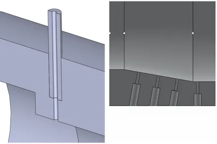
[image:39.595.97.515.189.400.2]

A diffuser with an angle of 4 degrees and 10 degrees with gas inlet will be used in this experiment. The diffusers will have the same geometry as the diffusers mentioned in Chapter 3.5, with the exception of several adjustments:

Figure 3.28: Cross-sectional view of the 10 degree diffuser with closed gas inlet.

Figure 3.29: Cross-sectional view of the 10 degree diffuser with open gas inlet.

• A gas inlet with a hole diameter of 7.5 mm will be placed 10 mm before the

diffuser entry. A pin can be placed inside this hole to block the gas inlet and test the diffuser without a gas inlet (Figure 3.28 and 3.29). This provides the possibility to compare the results with the results obtained from Experiment D.

• A 1 mm hole is drilled through the diffuser wall at each pressure tap location.

A 3 mm chamber is drilled on top of the 1 mm holes in which the pressure taps are mounted (Figure 3.30). The holes on the inside of the diffusers are cleared of any burrs. This ensures that the holes on the inside of the diffuser are as smooth as possible.

• Holes that are drilled on the oblique side of the diffuser are drilled

perpendicu-lar to the oblique side (Figure 3.31).

(40)

[image:40.595.68.507.84.376.2]

Figure 3.30: Cross-section of a pressure tap on the 10 degree dif-fuser.

Figure 3.31: Pressure tap holes drilled on the oblique side of the 10 degree diffuser.

is chosen based on the gas to air ratio used in appliances. The mass stoichiometric ratio is the ratio of oxidizer to fuel where all the fuel and oxidizer are used [19]. It is defined as: s= YO YF st

, with Yk = mk

mtotal (3.6)

WhereY0 and YF are the mass fractions of oxidizer and fuel, respectively. The

choice of gas and oxidizer (in this case air) will define the stoichiometric ratio. The equivalence ratio can then be defined as:

φ =sYF YO

(3.7) Appliances operate at an equivalence ratio lower than one. This implies that more air than needed for stoichiometric combustion is present in the air-gas mix-ture. This is done for safety reasons, since an equivalence ratio ofs >1will result in

incomplete combustion and thus the formation of carbon monoxide. An equivalence ratio which is too low is also unwanted, since it will result in acoustic instability of the burner flame (instable flame). At a certain value ofφ the flamability limit is reached.

(41)

3.6. EXPERIMENTE: DIFFUSER WITH GAS INLET 31

appliances is typically around 0.8. The combination of the equivalence ratio, appli-ance output power and type of gas result in values for the mass flow of the gas and air. Choosing an output power of 30kW (which is typical for a regular household), G20 gas and atmospheric operating conditions results in the following mass flow rates of unburnt gas and air:

˙

mgas = 6.0403·10−4 kg/s mair˙ = 1.2990·10−2 kg/s (3.8)

The mass flow of air is generated by the fan and can be monitored with the orifice flow meter. The mass flow of gas is generated by the underpressure which is present before the diffuser entry. A hole is drilled at the location at which the gas is to be injected, on which a tube is mounted. This tube will ensure a better developed entry flow. The inlet length of the tube is chosen to be 10 pipe diameters. No extra flow meter is used to measure the mass flow rate of the gas or the total mass flow rate. Instead, the mass flow is estimated based on the amount of underpressure at the gas inlet location, the hole diameter and the amount of resistance the tube for the gas inlet will generate. Also, the G20 gas is replaced by air for practical reasons. This will result in different behavior of the flow inside the diffuser due to the difference in density, viscosity and amount of mass flow. The goal of the measurements is to validate simulations, which will also be performed with air as a replacement for gas.

Figure 3.32: Schematic of the diffuser set-up with gas inlet.

The hole diameter needed to achieve a mass flow of 6.0403·10−4 kg/s of air at

the inlet can be estimated by analysing the static pressure at the gas inlet location from previous experiments at a flow rate of 1.2990·10−2 kg/s. The location of the

gas inlet is chosen to be 1 cm upstream of the diffuser entry. In experiment D, at

ReD = 40280 the mass flow rate was1.117·10−2 kg/s for the 4 degree diffuser. The

(42)

-438 Pa compared to the ambient pressure. The hole diameter can be determined by applying Bernoulli’s equation:

p1 + 0.5ρv12 =p2+ 0.5ρv22 (3.9)

Where0.5ρv2 is the dynamic pressure. Figure 3.32 shows that the dynamic

pres-sure at location 1 is zero, since the velocity in the y-direction is zero. At location 2, the static pressure is assumed to be ambient. This results in:

p1 =pambient+ 0.5ρv22 (3.10)

p1−pambient = 0.5·1.2∗v22 =−438 (3.11)

The negative pressure indicates thev2 operates in negative y-direction.

v2 =

r

438

0.6 ≈27m/s (3.12)

The gas inlet diameterDg follows from the known mass flow rate:

˙

m= 0.25πd

2_v ρ (3.13) Dg = r ˙ mρ

0.25πv ≈5.84mm (3.14)

Since this calculated diameter does not include the pressure loss that occurs in the pipe, this diameter will have to be larger in reality. An estimation of the pressure loss can be made by assuming a pipe with a diameter of 5.8 mm and length of 58 mm (10 pipe diameters). Applying the Darcy-Weisbach equation gives the amount of pressure loss:

∆P =f L

Dg ρv2_avg

2 ≈136.09Pa (3.15)

This value can be added to the static pressure used in Equation 3.11 to correct for the pressure loss due to skin friction. Equation 3.12 to 3.14 can be re-evaluated to obtain a new value for the diameter: Dg = 6.5mm.

(43)

3.7. EXPERIMENTF: DIFFUSER WITHOUT GAS INLET,EXTRA PRESSURE TAPS 33

3.7 Experiment F: Diffuser without gas inlet, extra

pressure taps

The results of Experiment D and E showed deviations from the simulations and theory upstream of the diffuser entry. To investigate this behavior further, some extra pressure taps were mounted upstream of the entry of the diffuser. The locations of these taps can be found in Figure 3.33. The location of the first and last pressure tap and the diffuser entry and exit can be found in Figure 3.34 to 3.36, where x = 0 mm is the position of the first pressure tap. The exact position of each pressure tap can be found in Appendix B.

The diffuser of 10 degrees showed no real signs of flow separation, since the theoretical pressure loss (without flow separation) matched the pressure loss of the simulations and measurements. For this reason an extra diffuser was made with an angle of 20 degrees. The expectation is that this diffuser will experience flow sep-aration. This way the accuracy of the simulations where flow separation is present can be tested. Detailed drawings of the 20 degree diffuser can be found in Appendix A.

(44)

Figure 3.34: Geometry of the test section containing the static pressure taps with 4 degree diffuser.

Figure 3.35: Geometry of the test section containing the static pressure taps with 10 degree diffuser.

(45)

3.8. EXPERIMENTG: WB6VENTURI 35

3.8 Experiment G: WB6 venturi

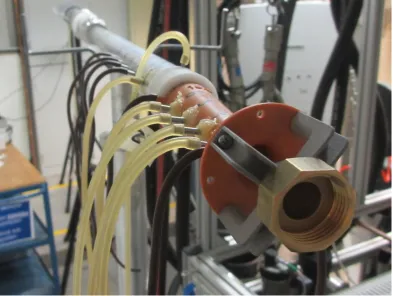
The next step is to measure an actual venturi which is used in the WB6 project. The venturi has a throat diameter of either 15.0 mm or 15.3 mm and a removable gas injection (Figure 3.37 and 3.38). In this experiment, air is used instead of gas through the gas inlet for practical reasons. The venturi will be tested both with and without gas inlet. The experimental set-up can be seen in Figure 3.39. In contrast to Experiment D to F, air enters the set-up through the venturi and exits the set-up through the fan. The reason for this is that the exit of the venturi has the same diameter as the end of the main set-up and that the gas injection is fitted to the entry of the venturi. A total of seven pressure taps are located on the wall of the venturi. Six more pressure taps are present at the section of tube downstream of the venturi.

Figure 3.37: 15.3 mm WB6 venturi with gas injection.

(46)

[image:46.595.89.483.264.560.2]

(47)

Chapter 4

Results

The next Chapters will discuss the results of the experiments mentioned in Chapter 3.

[image:47.595.98.531.391.655.2]

4.1 Experiment A: PVC pipe

Figure 4.1: Pressure drop over the first section of PVC pipe versus the Reynolds number.

The pressure at different locations on the pipe was measured at different Reynolds numbers. The locations of the static pressure taps can be found in Figure 3.12. Dif-ferent measurements were performed at fan output powers ranging from 30% to

(48)

[image:48.595.199.373.86.258.2]

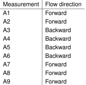
Measurement Flow direction A1 Forward A2 Forward A3 Backward A4 Backward A5 Backward A6 Backward A7 Forward A8 Forward A9 Forward

Table 4.1: Configurations during each PVC pipe measurement.

100%, at intervals of 10%. At fan output powers below 30%the mass flow

measure-ment in the orifice meter became inaccurate due to the fact that the fluctuations in the pressure readout were high in comparison with the pressure drop over the orifice meter. Before each measurement the ambient air temperature and pressure were determined to calculate the air density. An overview of the configuration of each measurement can be found in Table 4.1. The fan blows air into the experimental set-up during the first two measurements, which will be referred to as measurements with forward flow. For measurement A3 to A6 the fan and thus the flow direction was reversed. The flow then enters the set-up at the end of the PVC pipe and exits through the fan. This will be referred to as measurements with backward flow. The pressure drop from the first to the second tap and from the second to the third tap are plotted versus the Reynolds number. The results can be found in Figure 4.1 and 4.2. The pressure drop from the first to the last tap versus the Reynolds number can be found in Figure 4.3. The Reynolds number ReD corresponds to the Reynolds in

the test section, whereD is the diameter of the PVC tube. The atmospheric

condi-tions during each measurement can be found in Table 4.2. Figure 4.4 to 4.6 show the absolute difference between the theoretical pressure drop and the measured pressure drop plotted versus the Reynolds number.

(49)

4.1. EXPERIMENTA: PVCPIPE 39

Property Dynamic

viscosity

Specific gas

constant Pressure Temperature Density

Symbol µ Rs P T ρ

Unit Pa s J kg−1_K−1 _Pa _K _{kg m}−3

Measurement A1 1.79·10−5 ₂₈₇ ₁₀₁₁₀₀ _293.15 _1.202

Measurement A2 1.79·10−5 ₂₈₇ ₁₀₁₁₀₀ _293.15 _1.202

Measurement A3 1.79·10−5 ₂₈₇ ₁₀₁₈₀₀ _293.85 _1.207

Measurement A4 1.79·10−5 ₂₈₇ ₁₀₁₈₀₀ _293.85 _1.207

Measurement A5 1.79·10−5 ₂₈₇ ₁₀₁₈₀₀ _293.85 _1.207

Measurement A6 1.79·10−5 ₂₈₇ ₁₀₁₈₀₀ _293.85 _1.207 Table 4.2: Atmospheric conditions during experiment A

that the measured pressure drop over 1 meter is more accurate than the measured pressure drop over 0.5 meter. The difference between each measurement is quite large. No clear conclusion can be drawn as to which measurement shows the best results.

During each measurement the problem occurred that the set-up was disturbed each time the manometer was connected to another pressure tap. This caused the set-up to move at connection points, resulting in small gaps through which the airflow could escape. These gaps cause a deviation in the volume flow calculated by the orifice meter. For the next measurement, any connection in the set-up was properly sealed with aluminum tape and a long and flexible plastic tube was connected to each pressure tap, which could be sealed with a plug. A total of three measurements was performed over a range of Reynolds numbers. The results can be seen in Figure 4.7 and 4.8. The configuration during the measurements can be found in Table 4.1. The absolute difference between the theoretical and measured pressure drop can be found in Figure 4.10 to 4.12.

(50)

[image:50.595.69.501.91.356.2]

Figure 4.2: Pressure drop over the second section of PVC pipe versus the Reynolds number.

(51)

[image:51.595.99.530.100.366.2]

Figure 4.3: Pressure drop over 1 meter of PVC pipe versus the Reynolds number.

[image:51.595.97.531.438.703.2]

(52)

[image:52.595.69.501.94.364.2]

Figure 4.5: Absolute difference between theoretical and measured pressure drop versus the Reynolds number.

[image:52.595.69.503.442.708.2]

(53)

[image:53.595.99.530.263.532.2]

(54)

[image:54.595.72.500.262.530.2]

(55)

[image:55.595.100.527.90.361.2]

Figure 4.9: Pressure drop over 1 meter of PVC pipe with improved set-up versus the Reynolds number. The Reynolds number is determined at the test section.

[image:55.595.97.530.445.714.2]

(56)

[image:56.595.70.499.93.365.2]

Figure 4.11: Absolute difference between theoretical and measured pressure drop versus the Reynolds number.

[image:56.595.69.501.441.708.2]

(57)

4.2 Experiment B: Copper pipe

Measurement Flow direction Adjustments B1 Backward

-B2 Forward

-B3 Forward

Tubes are fitted to each pressure tap to prevent any movement of the experimental set-up when the manometer is fitted to another pressure tap

B4 Backward

-B5 Forward Any possible gaps in the set-up are made airtight.

B6 Backward

-Table 4.3: Configurations during each copper pipe measurement.

The second measurement was performed with the copper pipe shown in Figure 3.14. The pressure at different locations on the pipe was measured at the same fan output powers as in Experiment A. A total of six measurements was performed at a range of flowrates. After each measurement several adjustments were made to the set-up. An overview of these adjustments can be found in Table 4.3. The internal diameter of the pipe was determined by measuring the internal diameter of 10 small pieces of pipe (Figure 4.13). The diameter was measured at both ends of each piece of pipe. The results can be found in Table 4.7. The average of these values, Davg = 20.064 mm, is taken as the internal diameter of the pipe.

During measurement B1 and B2, the pressure taps that were not connected to a manometer were sealed with pieces of plastic tubing. The problem with this

config-Property Dynamic

viscosity

Specific gas

Measurement B1 1.79·10−5 ₂₈₇ ₁₀₁₈₀₀ _293.85 _1.207

Measurement B2 1.79·10−5 ₂₈₇ ₉₉₁₀₀ _293.65 _1.176

Measurement B3 1.79·10−5 ₂₈₇ ₁₀₀₂₀₀ _293.35 _1.190

Measurement B4 1.79·10−5 ₂₈₇ ₁₀₀₂₀₀ _293.35 _1.190

Measurement B5 1.79·10−5 ₂₈₇ ₁₀₃₄₀₀ _293.55 _1.227

(58)

[image:58.595.115.456.86.312.2]

Figure 4.13: Copper pipe samples.

uration is that the set-up was disturbed each time the manometer was connected to another pressure tap, as explained in Experiment A. This effect was again limited by fitting long plastic tubes to each pressure tap that could be closed with a plug. For measurement B5 and B6, any possible gaps in the connections of the set-up were made airtight by applying aluminum tape. Gaps in the set-up can result in pressure drops and errors in the measurement of the volume flow. The measured pressure drop from 0.0 m to 0.8 m and from 0.8 m to 1.6 m can be found in Figure 4.14 and 4.15. For the section from 0.0 m to 0.8 m the entry length is 0.2 m and the exit length 1.1 m. From 0.8 m to 1.6 m the entry length is 1.0 m and the exit length is 0.3 m. The pressure drop from the first to the last tap can be found in Figure 4.16. The pressure drop over each segment of 0.2 m can be found in Figure 4.17 to 4.25. The Reynolds numberReD corresponds to the Reynolds number in the test section, whereDis the

diameter of the copper pipe. The atmospheric conditions during each measurement can be found in Table 4.4.

(59)

[image:59.595.100.530.91.358.2]

Figure 4.14: Pressure drop from 0.0 m to 0.8 m versus the Reynolds number. The Reynolds number is determined at the test section.

(60)

[image:60.595.68.504.95.363.2]

Figure 4.15: Pressure drop from 0.8 m to 1.6 m versus the Reynolds number. The Reynolds number is determined at the test section.

[image:60.595.72.503.445.713.2]

(61)

[image:61.595.99.530.96.365.2]

Figure 4.17: Pressure drop from 0.0 m to 0.2 m versus the Reynolds number for the copper pipe.

[image:61.595.99.530.442.710.2]

(62)

[image:62.595.70.505.95.366.2]

[image:62.595.69.503.442.708.2]

(63)

[image:63.595.99.531.96.365.2]

[image:63.595.98.532.441.710.2]

(64)

[image:64.595.71.503.97.364.2]

[image:64.595.68.503.442.709.2]

(65)

[image:65.595.100.531.273.537.2]

(66)

4.3 Experiment C: Copper pipe with grid

The measurement procedure in this experiment was similar to the procedure in Chapter 4.2. The flow direction will be forward since this configuration showed the best results in Experiment B. The pressure drop from 0.0 m to 0.8 m and from 0.8 m to 1.6 m can be found in Figure 4.26 and 4.27. The pressure drop over the entire pipe can be found in Figure 4.28. The pressure drop over each section of 0.2 m can be found in Figure 4.29 to 4.37. The atmospheric conditions during each measure-ment can be found in Table 4.6. The configuration during each measuremeasure-ment can be found in Table 4.5.

Measurement Flow direction Grid type C1 Forward Fine grid C2 Forward Coarse grid C3 Forward No grid

Table 4.5: Configurations during Experiment C.

viscosity

Specific gas

Measurement C1 1.79·10−5 287 100400 293.25 1.193

Measurement C2 1.79·10−5 287 100400 293.25 1.193

Measurement C3 1.79·10−5 287 100400 293.25 1.193 Table 4.6: Atmospheric conditions during experiment C.

(67)

4.3. EXPERIMENTC: COPPER PIPE WITH GRID 57

Figure 4.26: Pressure drop from 0.0 m to 0.8 m of versus the Reynolds number, copper pipe with and without grids. The Reynolds number is deter-mined at the test section.

measurements do not show a significant effect on the entry length needed for pre-cise pressure measurements. For the section (0.0 m to 0.8 m) the entry length is 10 diameters. For the second section of pipe (0.8 m to 1.6 m), the entry length is 50 di-ameters. Figure 4.29 to 4.37 show that there is still a large variation in the pressure drop per section of 0.2 m.

The reason that the effect of the grids cannot be noticed may be due to the fact that more screens and a honeycomb are needed in the presence of a settling chamber to effectively create a homogeneous flow in the test section. One grid may not be enough to achieve a noticeable improvement as it is located far away from the test section. Detailed velocity analyses should be performed to properly investigate the effect of the grid.

4.3.1 Error estimation

(68)

Figure 4.27: Pressure drop from 0.8 m to 1.6 m of versus the Reynolds number, copper pipe with and without grids. The Reynolds number is deter-mined at the test section.

roughness heightare not taken into account in the errobars because they are hard

to quantify. The error in the internal diameter of the copper pipe was determined by taking the minimum and maximum found in Table 4.7, and subtracting them from the average value of 20.06 mm. This results in an error of -0.094 mm and +0.076 mm. These errors have an effect on the theoretical pressure drop, but also on the flow rate and the Reynolds number. The error in the Reynolds number is small how-ever, less than 1 percent at most. The errors in the pressure readout are mainly due to fluctuations in the pressure displayed by the manometers. The TT series micro-manometer had a readout error ranging between 0.5 Pa and 2.0 Pa, depending on the Reynolds number. The error in the readout of the Neotronics micromanometer ranged between 0.2 and 1 mmH20. Multiplying by a factor 9.81 gives the pressure

in Pascals. This results in an error of approximately 2 to 10 Pa. The resolution of the manometers is negligible in comparison with the error in the readout (± 0.05 Pa).

(69)

Figure 4.28: Pressure drop over 1.8 meter versus the Reynolds number, copper pipe with and without grids. The Reynolds number is determined at the test section.

(70)

Figure 4.30: Pressure drop from 0.2 m to 0.4 m versus the Reynolds number for the copper pipe with and without grids.

(71)

(72)

(73)

(74)

Tube number 1 2 3 4 5 Diameter 1 (mm) 20.02 20.06 20.05 20.07 20.14 Diameter 2 (mm) 20.05 20.0 20.04 19.97 20.13 Tube number 6 7 8 9 10 Diameter 1 (mm) 20.09 20.12 20.04 20.01 20.12 Diameter 2 (mm) 20.05 20.11 20.09 20.04 20.08

Table 4.7: Internal diameter of the copper tube. Diameters 1 and 2 correspond to diameters at both ends of the tubes.

Error source Parameter Approximate error

PVC pipe dimension

Variation in diameter ±0.2 mm

Theoretical pressure drop Depending on flow rate, ranging from 20 to 90 Pa Reynolds number <1 percent

Copper pipe dimensions

Variation in diameter +0.076 mm, -0.094 mm Theoretical pressure drop Depending on flow rate,

ranging from 3 to 16 Pa/m Reynolds number <1 percent

Pressure taps Pressure Unknown

Orifice meter Internal error Unknown Readout error ±1 Pa

Manometers Resolution ±0.05 Pa

Readout error Depending on flow rate, ranging from 0.5 to 10 Pa

(75)

4.4. EXPERIMENTD, EAND F,NO INJECTION 65

4.4 Experiment D, E and F, no injection

The static pressure in the diffusers without air injection was measured at three differ-ent Reynolds numbers for all three experimdiffer-ents. The Reynolds numbers (ReD) are

determined at the entry of the diffuser, which has a diameter of D = 30 mm. One

Reynolds number should be approximately 55000 to be able to compare the mea-surement to the experiments of Sprenger [8]. The resulting pressure distributions are compared to the theoretical pressure distributions and simulations. Chapter 4.4.1 to 4.4.3 will show the results for the 4, 10 and 20 degree diffusers. The theo-retical pressure distribution includes the pressure increase in the diffuser according to Bernoulli’s equation and pressure losses due to skin friction, where the pressure is assumed to be atmospheric at the exit of the set-up. Pressure losses due to pos-sible flow separation are not taken into account. The corresponding geometries of the test sections containing the 4, 10 and 20 degree diffuser can be found in Figure 4.38, 4.48 and 4.58. The atmospheric conditions during each measurement can be found in Table 4.9.

Simulations were performed in ANSYS Fluent using a standard k−turbulence

model with enhanced wall treatment and axisymmetric geometry [20]. In addition, simulations on the 20 degree diffusers at the lowest Reynolds number were also performed using a realisable k− model and Reynolds stress model. The reason

for this is that the standardk− model did not show the same amount of pressure

drop as in the measurements. The meshes and resulting pressure and velocity distributions in the diffuser can be found in Chapter 4.4.1 to 4.4.3.

viscosity

Specific gas

Experiment D 4◦ _NI ₁_.₇₉_·₁₀−5 ₂₈₇ ₁₀₁₂₀₀ _293.55 _1.201

Experiment D 10◦ _NI ₁_.₇₉_·₁₀−5 ₂₈₇ ₁₀₁₉₀₀ _293.25 _1.211

Experiment E 4◦ _NI ₁_.₇₉_·₁₀−5 ₂₈₇ ₁₀₂₂₀₀ _293.25 _1.214

Experiment E 10◦ _NI ₁_.₇₉_·₁₀−5 ₂₈₇ ₁₀₁₉₀₀ _293.85 _1.208

Experiment F 4◦ _NI ₁_.₇₉_·₁₀−5 ₂₈₇ ₁₀₂₂₀₀ _293.25 _1.214

Experiment F 10◦ _NI ₁_.₇₉_·₁₀−5 ₂₈₇ ₁₀₁₁₀₀ _293.25 _1.201

Experiment F 20◦ _NI ₁_.₇₉_·₁₀−5 ₂₈₇ ₁₀₀₅₀₀ _293.55 _1.193 Table 4.9: Atmospheric conditions during experiment D, E and F without air injection

(76)

4.4.1 4 Degree diffuser

Figure 4.38: Geometry of the test section with the 4 degree diffuser.

Figure 4.39: Mesh for the simulation of the 4 degree diffuser.

(77)

Figure 4.41: Velocity distribution in the 4 degree diffuser, ReD = 52980.

Figure 4.42: Static pressure distribution in the 4 degree diffuser,ReD = 52980.

Figure 4.43: Velocity distribution in the 4 degree diffuser, zoomed in around the diffuser entry,

ReD = 52980.

(78)

Figure 4.45: _{Static pressure versus length, 4 degree diffuser. ReD corresponds to}

the Reynolds number at the diffuser entry.

(79)

(80)

4.4.2 10 Degree diffuser

Figure 4.49: Mesh for the simulation of the 10 degree diffuser.

(81)

Figure 4.51:Velocity distribution in the 10 degree diffuser, ReD = 52230.

Figure 4.52: Static pressure distribution in the 10 degree diffuser, ReD = 52230.

Figure 4.53: Velocity distribution in the 10 degree diffuser, zoomed in around the diffuser entry,

ReD = 52230.

(82)

(83)

(84)

4.4.3 20 Degree diffuser

(85)

(86)

4.4.4 Discussion

Figure 4.62: Streamlines in a diffuser without viscous effects.

Figure 4.63: Streamlines in a diffuser with viscous effects.

(87)

locally around the entry before it increases in the diffuser itself. This effect can also be noticed in Figure 4.43, 4.44, 4.53 and 4.54.

The pressure increase in the diffuser itself is also different in theory than it is in measurements and simulations. The reason for this behavior can be explained by looking at the velocity profiles along the cross-section of the diffuser (Figure 4.41 and 4.51). When the flow enters the diffuser the bulk flow wants to follow a straight path and does not evenly spread in the diffuser. This will cause the velocity to be lower at the wall of the diffuser than it would be in the ideal case where the velocity profile across the diffuser is fully developed. It will take a certain length of pipe for the velocity profile to be fully developed again. This effect becomes easier to notice when the diverging angle of the diffuser becomes larger, as can be seen in the resulting pressure distribution for the 4, 10 and 20 degree diffuser.

The pressure drop in the 20 degree diffuser shows larger values for the pressure drop in experiment than the theory and simulations predicted. This is due to the presence of flow separation. The realisable k − shows slightly more pressure

drop than the standardk −model. The Reynolds stress model shows even more

pressure drop. However, the pressure distribution in the tube before the diffuser entry deviates from the theoretical and measured pressure distribution.

(88)

Experiment E and F showed a slight increase in pressure upstream of the dif-fuser entry before the drop in pressure at the difdif-fuser entry (Figure 4.64). This was not the case for experiment D. The reason for this behavior is probably due to slight differences in the geometry of both diffusers. Measurements with a caliper showed that the diameter of the entry tube was approximately 29.7 mm, whereas the diam-eter of the diffuser entry of Experiment E and F was approximately 30.0 mm. The transition from pipe to diffuser is located at a distance of 255 mm. This transition in diameters explains the slight increase in pressure. This also means that the pres-sure from 0 mm to 230 mm in the plots of the prespres-sure in the 4, 10 and 20 degree diffuser will be slightly higher if the entry tube has a diameter of exactly 30 mm. This also means the difference between the simulations and measurements will be slightly higher. The extra amount of pressure loss can be accredited to the fact that the inside of the diffuser is not smooth. The extra amount of roughness heightwill

result in more pressure loss due to skin friction.

To compare the results of the 4 degree diffuser with the diffuser from the exper-iments of Sprenger [8] and the 10 degree diffuser, the pressure and position in the diffuser can be written in a dimensionless form as described in Chapter 2.2. The position in the diffuser can be written in dimensionless form by dividing the diffuser diameter at location x by the diffuser diameter at the entry (Dx/DE). Figure 4.65

shows a plot of the dimensionless pressure versus the dimensionless position in the diffuser. PE is measured at the pressure tap at L = 274 mm (6 mm before the diffuser

entry) for experiment E and F (Figure 4.46). The entry pressure for Experiment D is hard to determine since there are a lot of fluctuations around the entry. It is taken at L = 278 mm, so 2 mm before the diffuser entry.

(89)

Figure 4.65: Dimensionless pressure versus dimensionless position for the 4 de-gree diffuser.

Experimental validation of simulations on flow through venturis and diffusers

Faculty of Engineering Technology