University of Warwick institutional repository: http://go.warwick.ac.uk/wrap
This paper is made available online in accordance with
publisher policies. Please scroll down to view the document
itself. Please refer to the repository record for this item and our
policy information available from the repository home page for
further information.
To see the final version of this paper please visit the publisher’s website.
Access to the published version may require a subscription.
Author(s): DWIGHT BARKLEY, M. GABRIELA M. GOMES and
RONALD D. HENDERSON
Article Title: Three-dimensional instability in flow over a backward-facing
step
Year of publication: 2002
Link to published version:
DOI: 10.1017/S002211200200232X Printed in the United Kingdom
Three-dimensional instability in flow over a
backward-facing step
By D W I G H T B A R K L E Y1, M. G A B R I E L A M. G O M E S1 AND R O N A L D D. H E N D E R S O N2
1Mathematics Institute, University of Warwick, Coventry CV4 7AL, UK 2Aeronautics and Applied Mathematics, California Institute of Technology,
Pasadena, CA 91125, USA
(Received 10 April 2002 and in revised form 1 July 2002)
Results are reported from a three-dimensional computational stability analysis of flow over a backward-facing step with an expansion ratio (outlet to inlet height) of 2 at Reynolds numbers between 450 and 1050. The analysis shows that the first absolute linear instability of the steady two-dimensional flow is a steady three-dimensional bifurcation at a critical Reynolds number of 748. The critical eigenmode is localized to the primary separation bubble and has a flat roll structure with a spanwise wavelength of 6.9 step heights. The system is further shown to be absolutely stable to two-dimensional perturbations up to a Reynolds number of 1500. Stability spectra and visualizations of the global modes of the system are presented for representative Reynolds numbers.
1. Introduction
The two-dimensional, absolute, linear stability of this flow has been examined extensively and is discussed in several publications (Gartling 1990; Greshoet al. 1993; Fortin et al. 1997). Computational studies have established that the two-dimensional laminar flow is linearly stable with respect to two-dimensional perturbations up to a Reynolds number of at least Re= 600. (As discussed in §2, several definitions of the Reynolds number are used in the literature. Appropriate reference scales for this problem are the upstream centreline velocity U∞ and step height h; all cited results
are expressed in these units.) However, additional computational evidence supports the existence of a local convective instability (again to two-dimensional disturbances) for a sizable portion of the domain at Reynolds numbers above 525 (Kaiktsis et al. 1996).
Denham & Patrick (1974) conducted experiments on laminar flow over a backward-facing step with an expansion ratio of 3. Velocity profiles and reattachment lengths of the primary recirculation zone were measured in the steady two-dimensional regime for Reynolds numbers up to 344. Denham & Patrick also describe transient three-dimensional flows within the primary recirculation zone following perturbations (obtained by tapping the channel) at Re= 344. Experiments by Armalyet al. (1983) on air flow in a backward-facing step geometry with nominal expansion ratio of approximately 2 provide quantitative measurements of two- and three-dimensional flows over a large range of Reynolds number, from about 50 to 6000. In addition to providing data on separation and reattachment points, streamwise velocity measure-ments are reported for several Reynolds numbers throughout the range of the study. Below Reynolds number 300 the flow is essentially spanwise invariant, although some deviation from two-dimensionality necessarily exists near the lateral sidewalls of the channel (see below). Above Re = 300 there is a measurable deviation from two-dimensionality. At about the same Reynolds number a secondary separation bubble is observed on the upper wall of the channel (the wall opposite the step).
Ghia et al. (1989) computed two-dimensional solutions of the backward-facing step flow throughout the laminar regime and found good agreement with the two-dimensional flows observed by Armalyet al. (1983). They discuss two mechanisms for the onset of three-dimensionality based on available information. They postulate that instability of the two-dimensional flow could result from a Taylor–G¨ortler instability after the formation of the secondary separation bubble on the upper wall because the main flow is then subject to destabilizing concave curvature. They also consider, but reject, the possibility that the sidewall boundary layer contributes to three-dimensional transition. Kaiktsiset al. (1991) studied the onset of three-dimensionality using direct numerical simulations, primarily for the case of a spanwise-periodic domain. They reported both two- and three-dimensional instability (unsteadiness) at approximately the same Reynolds number: Re'525. However, Kaiktsiset al. (1996) later showed that this two-dimensional instability was convective rather than absolute. They report that the three-dimensional instability occurs at the ‘boundaries between the primary and secondary recirculation zones with the main channel flow’.
plane’. The implication is that the three-dimensionality observed in the experiments results from an extrinsic effect induced by the lateral boundary conditions, and thus will probably depend on the system aspect ratio. The observed three-dimensionality does not follow from a fundamental hydrodynamic instability of a two-dimensional flow.
Thus in spite of the numerous investigations of flow over a backward-facing step available in the literature, some of the most basic questions for this flow remain open: in the ideal problem with no sidewalls, at what Reynolds number does the flow first become linearly unstable, what is the nature of this instability, and where in the flow does it originate? These are the questions we wish to address. We focus on the accurate determination of the initial intrinsic three-dimensional instability. This is similar in spirit to the work of Kaiktsiset al. (1991) which attempted to quantify the transition to three-dimensionality in backward-facing step flow via direct numerical simulations. Our approach is a computational bifurcation analysis of the flow. We will show that the primary instability for the backward step flow is a three-dimensional, steady bifurcation.
Our presentation is organized as follows. In§§2 and 3 we formulate the problem and describe our numerical methods. In §4 we report the results of our stability analysis for Reynolds numbers up to 1050, and in §5 we discuss these results in the context of experiments and transition to turbulence for the flow over a backward-facing step.
2. Problem formulation
Consider the motion of a viscous fluid contained between two fixed plates with a step change in separation distance at the origin. We take the flow direction to be such that fluid moves toward the larger gap, i.e. a backward-facing step. The fluid is assumed to have constant densityρand constant kinematic viscosityν. The Reynolds number is Re ≡ UrefLref/ν, where the reference scales Lref and Uref for length and
velocity are specified below.
The fluid motion is governed by the incompressible Navier–Stokes equations, written in non-dimensional form as
∂u
∂t =N(u)−∇p+ 1
Re∇2u in Ω, (2.1a)
∇ ·u= 0 in Ω, (2.1b)
where u(x, t) is the velocity field,p(x, t) is the static pressure,Ω is the computational domain, and N(u) represents the nonlinear advection term:
N(u)≡ −(u· ∇)u. (2.1c)
αh
h x
y
z
Li Lo Lz
(1 + α)h
Figure 1.Flow geometry for the backward-facing step. The origin of the coordinate system is at the step edge. In this work we take the ratio of inlet height to step height asα= 1, so that the expansion ratio is 1 + 1/α= 2.
range 15h6Lo 655h. Finally we take the system to be homogeneous in the spanwise direction and we take the system to be infinitely large in this direction, i.e. Lz = ∞, by considering all spanwise Fourier modes (see §3).
Boundary conditions are imposed on the flow as follows. At the inflow boundary (x=−Li, 06y6αh) we impose a parabolic profile:u= 4y(αh−y)/(αh)2,v=w= 0. Along the step and all channel walls we impose no-slip conditions. At the outflow boundary (x=Lo, −h6y 6αh) we impose a standard outflow boundary condition for velocity and pressure:
∂xu(x, t) = (0,0,0), p(x, t) = 0. (2.2) Along all other boundaries the pressure is forced to satisfy the high-order Neumann boundary condition given by Karniadakis, Israeli & Orszag (1991).
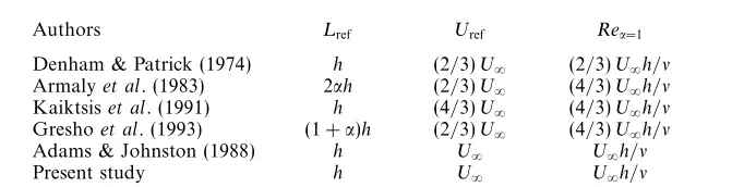
Several different choices of non-dimensionalization appear in the literature. Table 1 provides a representative list of reference scales,Lref andUref, and the corresponding
Reynolds number in the case α = 1. The step height h is a natural length scale for defining the problem geometry and measuring quantities like downstream separation points, and it is the most common choice for Lref. Other common length scales used
are the downstream channel height (1 +α)hor, if the incoming flow is turbulent, the momentum thickness of the upstream boundary layer. Two different velocity scales are commonly used: the maximum upstream centreline velocity U∞ and the average
upstream velocity U:
U= αh1 Z αh
0 u(y) dy.
Note that U = (2/3)U∞ for parabolic inflow velocity. In the present work we take
Lref =handUref =U∞, giving the Reynolds number as
Re≡ U∞h
ν . (2.3)
This definition of Reynolds number is independent of α. All quantities cited from the literature (Reynolds numbers, separation points, velocities, eigenvalues, etc.) are rescaled using this non-dimensionalization.
3. Computational methods
Authors Lref Uref Reα=1
Denham & Patrick (1974) h (2/3)U∞ (2/3)U∞h/ν Armalyet al. (1983) 2αh (2/3)U∞ (4/3)U∞h/ν Kaiktsiset al. (1991) h (4/3)U∞ (4/3)U∞h/ν Greshoet al. (1993) (1 +α)h (2/3)U∞ (4/3)U∞h/ν Adams & Johnston (1988) h U∞ U∞h/ν
[image:6.595.135.476.139.225.2]Present study h U∞ U∞h/ν
Table 1.Comparison of reference scales used in various studies. The most common choice is the last one:Lref =h(step height) andUref =U∞(upstream centreline velocity). Different scalings lead to different definitions of the Reynolds number, tabulated forα= 1.
by Mamun & Tuckerman (1995), Barkley & Henderson (1996), and Barkley & Tuckerman (1999).
All of the calculations were carried out using a non-conforming spectral element program (Prism, Henderson 1994). In the spectral element method a two-dimensional domain Ω is represented by a mesh of K elements. Within each element both the geometry and the solution variables, in this case u(x, t) and p(x, t), are represented usingNth-order (Legendre) polynomial expansions. Figure 2 shows the basic compu-tational domains used for simulations of the backward-facing step flow over the entire range of Reynolds numbers. Non-conforming elements allow local mesh refinement in regions like the step corner yet preserve the block structure of the calculations. Computational domains with various refinement levels and outflow lengths were used at different Reynolds numbers and will be discussed in §3.3.1 below. Beyond the details of the polynomial basis and the treatment of non-conforming elements in the mesh, the method follows a standard Galerkin finite element procedure to discretize equation (2.1). Henderson & Karniadakis (1995) discuss further details of the method and solution techniques, along with various validation studies for the particular code employed here.
For the most part the method we use to study bifurcation problems does not depend on any particular spatial discretization so we can describe the relevant algorithms in the following abstract way. Let u(t) be the n-dimensional vector containing the discrete representation of the velocity field u(x, t). Discretizing the Navier–Stokes equations (2.1) gives a system of differential algebraic equations schematically of the form
du
dt =N(u) +Lu, (3.1)
whereL and N(·) are linear and nonlinear operators respectively. For linear stability and steady-state calculations we also require equations describing the linear evolution about some given reference state U. These equations take the form
du
dt = (NU+L)u, (3.2)
where NU is the linearization (Jacobian) of the operator N about state U. More specifically, letU +ube an infinitesimal perturbation to a steady flowU. Equations for the evolution of uare obtained by replacing the nonlinear advection term in the Navier–Stokes equations with the linearization
M1
M2
M4 M3a
M3b
" "
Figure 2.Computational domains used in the present study. Subscripts label external dimensions (specifically outflow lengthLo). Each domain is divided intoKelements. Where necessary, lower-case letters label the degree of internal mesh refinement: theM3amesh hasK= 83 elements and theM3b mesh hasK= 203 elements. Within each element the solution and geometry are represented byN2
polynomial coefficients. Two subsections of meshM4are expanded to show the internal distribution
of quadrature points for polynomial orderN= 7. To simulate a three-dimensional flow the solution is decomposed into M Fourier modes in the periodic spanwise direction, each computed on the same two-dimensional grid.
The boundary conditions for the perturbation u are the same as those for the base flow U except that u= 0 at the inlet. Therefore U +u satisfies the same boundary conditions asU.
Our primary tool is a method for evolving some given state forward in time. Define the operatorsAand AU as follows:
Au(t)≡u(t) + Z t+T
t (N(u) +Lu) dt
0, (3.3)
AUu(t)≡u(t) +
Z t+T
t (NU+L)udt
0. (3.4)
A gives the nonlinear evolution of u(t) over time interval T. It also represents our simulation code as a black box for integrating the Navier–Stokes equations: given a velocity field u(t), it provides the solution at a later time u(t+T) =Au(t). The operator AU gives the analogous linear evolution ofu(t) about some given reference state U. In practice both equations (3.1) and (3.2) are integrated using the third-order semi-implicit splitting scheme described by Karniadakis et al. (1991). For the remainder of this section, however, we will only refer to the operators A and AU rather than the time-dependent Navier–Stokes equations that they represent.
3.1. Steady-state calculations
is to use fixed-point iteration:
Uk+1 =AUk. (3.5)
If all eigenvalues µi ofAU satisfy|µi|<1, then the steady-state solutionU islinearly stable and the sequence converges, Uk→U, for most initial conditions. This is equivalent to performing time-integration. To accelerate convergence, once the initial (fast exponential) transients decay we switch to a Newton iteration:
(AUk−I)uk= (A−I)Uk, Uk+1=Uk−uk.
)
(3.6)
Each Newton iteration requires an inversion of the linear operator (AU−I). This is accomplished with a generalized minimum residual (GMRES) iterative method (Saad & Schultz 1986).
For moderate Reynolds numbers (up to Re≈800) our steady-state calculations for the backward-facing step flow consist of only a few explicit steps followed by Newton iterations. For the definition of the operators A and AU we use T equal to a typical time step (∆t= 5×10⁻³). For larger values of the Reynolds number
(Re>800) we typically find that the number of GMRES iterations necessary to invert (AU −I) becomes so large that simple fixed-point iteration (3.5) requires less computation time. The Stokes preconditioning method of Mamun & Tuckerman (1995) does not work in our case because our numerical operators derive from a third-order splitting scheme (Karniadakis et al. 1991) which does not impose exact incompressibility of the flow. The divergence of the velocity field is of order ∆t3,
which is acceptable in direct simulations or in our Newton’s method with ∆t small. However, in Mamun–Tuckerman preconditioning ∆tis large and so the divergence of the flow becomes very large and the numerical method fails. What this implies for the present study is that our method for computing steady states works well up to and slightly above the Reynolds number for the primary three-dimensional instability of the flow (§4.1). However our method is not well suited for larger Reynolds numbers, for example those which must be attained for two-dimensional linear instability of the flow (§4.3). We are able to obtain steady two-dimensional flows between Reynolds number 800 and 1500 only by fixed-point iteration (3.5), effectively time integration. This is feasible since the flows we consider are globally two-dimensionally stable, but the convergence is very slow due to the smallness of the leading two-dimensional eigenvalues (§4.3).
3.2. Stability analysis
For the linear stability calculations we need to solve the eigenvalue problemAUu˜=µu˜, where µis an eigenvalue of the operator AU and ˜u is the corresponding eigenmode. For a time-independent base flowU, the eigenvaluesσ+ iω of the linearized Navier– Stokes operator NU+L are related to the eigenvaluesµviaµ= exp((σ+ iω)T). An instability occurs ifσ >0 and the resulting bifurcation may be either steady (ω = 0) or oscillatory (ω6= 0).
Again we turn to iterative methods. Let u1 be some initial guess for the dominant
eigenmode of AU. To begin we generate the Krylov sequence
u1, u2=AUu1, u3=AUu2, . . . , um=AUum−1.
X=hu1, u2. . . umi. Next we execute the block power iteration
Xk+1=AUXk. (3.7)
Because Xk is a Krylov subspace, each iteration of (3.7) requires only a single matrix-vector multiplication to generate the next element of the sequence. Computing an orthonormal basis for the space Xk after each iteration gives estimates for the dominant eigenvalues and eigenmodes of AU. Any absolute global instability will necessarily be found by this method as long as u1 is not exactly orthogonal to
the unstable mode of the system. Not only is this very unlikely (and essentially impossible in the presence of random round-off errors), but in addition we often effectively generate several different choices for u1 at the same Reynolds number by
using different meshes.
For the backward-facing step problem we use a subspace dimension m typically between 20 and 80 and obtain highly accurate leading eigenvalues after O(100) subspace iterations. Typically 200 subspace iterations are required to obtain the four leading eigenvalues accurately. In defining the operator AU for these calculations we use an evolution time of T = 5. For more details and additional applications see Edwards et al. (1994), Mamun & Tuckerman (1995), Schatz, Barkley & Swinney (1995), and Barkley & Henderson (1996).
Our primary concern here is the three-dimensional stability of steady two-dimen-sional flows, and in this case the eigenmodes take a special form. Because the system is homogeneous in the spanwise direction, we can decompose general perturbations into Fourier modes with spanwise wavenumbersβ:
(u, p) = Z ∞
−∞( ˆu,pˆ) e
iβzdβ.
At linear order, modes with different |β| are decoupled. It follows directly from the linearized Navier–Stokes equations that any eigenmode of AU with a given β must be of the following form:
˜
u(x, y, z) = ( ˆu(x, y) cosβz,vˆ(x, y) cosβz,wˆ(x, y) sinβz), ˜
p(x, y, z) = ˆp(x, y) cosβz,
)
(3.8)
or an equivalent form obtained by translation in z. Restricting attention to modes with a particular β reduces the full three-dimensional stability problem at any given Reynolds number to a one-parameter family of problems for the Fourier components ( ˆu,v,ˆ wˆ) of the eigenmode u(˜ x, y, z). These Fourier components are computed on a two-dimensional domain withβappearing in the linearized equations as an additional parameter. Linearizing the equations in this way also frees us from the erroneous effects of imposing periodic boundary conditions with an incorrect length, since β can be varied continuously. Our stability calculations therefore produce a family of eigenvalues µ(β), or equivalently σ(β) + iω(β), for a discrete set of fixed Reynolds numbers.
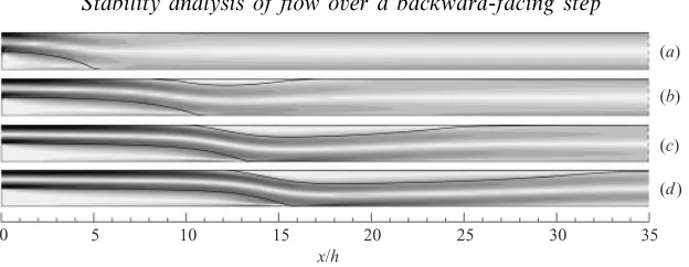
(a)
(b)
(c)
(d)
0 5 10 15 20 25 30 35
[image:10.595.142.454.117.238.2]x/h
Figure 3.Visualization of the steady two-dimensional base flows at (a) Re= 150, (b) 450, (c) 750 and (d) 1050. Each image shows the separation streamlines associated with the primary and secondary recirculation zones. Shaded regions correspond to vorticity magnitude in the range 0 6|ωh/U∞|62. Note the appearance of a separation bubble on the upper wall at Re'300 (between the (a) and (b)). The dashed lines on the right indicate the outflow boundary of the computational domain. For (d)Lo= 45hand the outflow boundary is outside the range shown.
3.3. Convergence tests
Flow past a backward-facing step is a deceptively difficult problem to fully resolve, especially at large Reynolds number. The combined effects of the geometric singularity at the step corner and the convective instability of the core flow can produce and then amplify numerical errors that mimic an intrinsic temporal flow instability. Gresho
et al. (1993) illustrate the minimum resolution requirements atRe= 600 for a variety of methods. In this section we outline our own convergence tests for both the base flow and stability calculations to establish that the numerical results we present are well-resolved.
3.3.1. Base flow
There are two central issues in checking convergence of the base flow calculations: external dimensions of the grid (Li and Lo) and the degree of internal refinement. External dimensions can be determined from a simple parameter study, but the unstructured nature of the discretization makes the internal refinement study more difficult to organize. Below we highlight only representative tests near the three-dimensional critical Reynolds number, although we did perform a large number of calculations to test both domain size and resolution over the full parameter range.
Figure 3 shows an overview of our base flow calculations in terms of steady-state vorticity fields and separation streamlines at various Reynolds numbers, and provides a qualitative picture of how the base-flow structure evolves with increasing Re. At moderate Reynolds number the steady flow consists of a primary separation bubble extending from the step and a secondary separation bubble that first appears on the upper wall at Re' 300. This secondary separation bubble was first reported by Armalyet al. (1983) and has been confirmed in numerous computational studies (e.g. Ghiaet al. 1989; Gartling 1990; Kaiktsiset al. 1991; Williams & Baker 1997).
The skin-friction coefficient, Cf, passes through zero exactly at the boundaries of the separation zones. This quantity provides a sensitive measure of the overall grid resolution. In the present case the skin-friction coefficient can be defined as
Cf ≡ −U2ν2 ∞
∂u ∂yny,
(a)
(b)
x/h x1
x2 x3
6
4
2
0
–2 (×10–3)
Cf
4
2
0
–2 (×10–3)
Cf
– 4
0 10 20 30
Figure 4. Computed skin-friction coefficients at Re= 750 along (a) the upper wall and (b) the lower wall of the channel. Solid circles (
•
) mark the three downstream locations whereCf(xj) = 0. Open circles () indicate results from a coarse grid, M3a with Nb = 7, while the solid lines (—) indicate results from a fine grid,M3b withNb= 7. Note the oscillations in the coarse-grid solution nearCf(x2); this is typical of a high-order method on an under-resolved grid.on the upper wall and ny =−1 on the lower wall. Although this quantity is only evaluated along the walls, its downstream distribution obviously depends on the dissipation of momentum in the core part of the flow. Figure 4 shows the computed distribution of Cf for both a coarse and fine grid calculation at Re = 750. The coarse and fine grids are based on the M3a and M3b meshes, respectively, shown in figure 2. Both calculations were run with a fixed polynomial order of Nb = 7. Even though the spectral-element method does not impose continuity of derivatives at element boundaries, continuous velocity gradients are obtained for sufficiently high polynomial order. This is evidenced by the fact that our Cf distributions appear continuous in the downstream direction. Oscillations in the solution along the upper wall suggest that the flow is ‘under-resolved’ on the coarse grid. These oscillations disappear upon grid refinement and the entire distribution converges to a smooth curve. Both solutions agree extremely well in the regions of the flow where Cf varies slowly.
[image:11.595.173.418.119.334.2]To further quantify the base flow calculations, we track the position of separation– reattachment points in the domain as a function of Reynolds number, i.e. the set of locations along the walls where Cf(xj) = 0. Figure 4 indicates the location of these points forRe= 750 based on the converged fine-grid solution. Since the extent of the primary and secondary separation zones varies with Reynolds number, the location of these points provides another good test of domain size and appropriate resolution. In particular it indicates the minimum external dimensions of the computational domain required to enclose the separation zones.
Figure 5 compares calculations on a variety of grids over the entire range of Reynolds number considered in our study. Our basic criterion for choosing Lo is to locate it five or more step heights downstream of the reattachment pointx3. We have
x/h x1
x2 x3
1500
Re
0 10 20 30
M1
Coarse
Fine 1000
500
40
M2 M3 M4
Figure 5. Separation–reattachment points in the backward-facing step flow as a function of Reynolds number. This figure compares results for several meshes with different geometries and internal levels of refinement. Dashed lines mark the location of the downstream boundary (Lo) for each mesh, with the vertical extent indicating the valid range inRefor each.
point for each consecutive grid pair. On the scale of the plot these overlaid points can barely be distinguished, thus showing that the computed reattachment points are insensitive toLo for the indicated Reynolds number range for each mesh. Consistent with the sensitivity of Cf shown in figure 4, the location of the separation point x2
does show some sensitivity to the degree of internal refinement, withx2 shifting just
slightly downstream on the finer grid.
The results in figure 5 agree well with published computational data. Below
Re= 300 the computed primary separation length also agrees with the experimental data of Armaly et al. (1983), although those experiments were performed with and expansion ratio of 1.94 rather 2. We also find that the secondary separation zone first appears at Re'300, as reported by Armaly et al. (1983). At larger Reynolds num-bers the primary separation length does not agree with the experimentally measured values because the experimental flow is three-dimensional. This effect is well docu-mented by Williams & Baker (1997). However, our results do agree well with other two-dimensional computations in this regime. In particular, Gartling (1990) reports from highly resolved computations that atRe= 600 these points occur atx1= 12.2,
x2= 9.7, and x3= 21.0. The corresponding values from our fine-grid calculations
are: x1 = 11.91, x2= 9.5, and x3= 20.6, giving a discrepancy of only about 2%.
Discrepancies at this level may be attributed to the slightly different inflow boundary conditions used in each calculation.
Nb Ne σ1 σ2 σ3 ω3 σ10
7 5 0.000129 −0.012811 −0.014109 0.031406 0.005919 7 7 0.000042 −0.012898 −0.014236 0.031633 0.004985 9 7 0.000033 −0.012966 −0.014234 0.031615 0.004927 9 9 0.000030 −0.012972 −0.014247 0.031615 0.004903
Table 2. Dependence of eigenvalues on polynomial order. Parameters Nb and Ne indicate the independent polynomial order of the base flow and eigenmode. Three leading eigenvalues computed on the meshM3b atRe= 750, β= 0.9 are given; the first two eigenvaluesσ1 andσ2 are real, the
third is complex:σ3±iω3. The leading eigenvalue σ10 computed on theM4 mesh at Re= 1050,
β= 1.5 is given in the last column.
refinement and recomputed these flows to generate fine-grid solutions at a few Reynolds numbers bracketing points of interest, e.g. the primary bifurcation.
3.3.2. Tests of stability calculations
To quantify the precision of eigenpairs (µ,u˜) produced by subspace iteration we compute the residual
r=kAUu˜−µ˜uk,
where k·k is the standard L2 vector norm and the eigenmodes are scaled so that
ku˜k= 1. In most cases we continue iterating until r <10−6 for one or more
eigen-modes, although in calculations that generate several modes the residuals for the dominant ones are orders of magnitude smaller than this. For practical purposes these can be considered exact eigenvalues of the operator AU so that the true accu-racy is determined by how well the numerical operator AU approximates the linear stability operator for the continuous problem.
Since accurate eigenvalue computations are predicated on having an accurate base flow U, the grid requirements (external dimensions and level of internal refinement) are dictated to a large degree by the base flow considerations discussed previously. However, we frequently use a lower polynomial order for the stability computations, particularly when scanning a large range of spanwise wavenumbers for a fixed base flow.
To demonstrate the accuracy of the eigenvalue computations, we present in table 2 results as a function of base flow and eigenmode polynomial order, Nb and Ne. We give the leading eigenvalues at Re= 750, β= 0.9, values extremely close to the primary instability, and also atRe= 1050,β= 1.5, values near those giving the largest growth rate found in our study. In all cases the residual satisfies r < 10−8 for the
leading eigenvalues σ1 and σ10, and satisfies r <10−6 for the other eigenvalues. The
eigenvalues have converged to an absolute accuracy of less than 10−4 at the highest
resolution (Nb=Ne= 9). The relative error ofσ1 in table 2 is large (becauseσ1≈0),
but the absolute error is small and sufficient to determine the primary instability to high precision.
backward-facing step geometry.† Such good agreement with an independent cal-culation – a relative difference less than 0.2% – gives us further confidence in our results.
Finally, as a test of the effect of outflow length on the stability computations we have computed the leading eigenvalue atRe= 1050 forβ= 0 andNb=Ne= 9 using two outflow lengths. For the M4 mesh (outflow L0 = 45) we obtain σ=−0.002896.
For a similar mesh with outflow L0 = 55 we obtain σ = −0.002904, thus verifying
that, just as for the base flow, L0 = 45 gives a well-resolved result at this Reynolds
number.
Our stability computations follow a similar protocol to that used for obtaining converged base flows. We initially compute eigenvalue branches using a moderate resolution. Typically we use theM3b mesh with polynomial ordersNb= 7 andNe= 7. Once the approximate location of a bifurcation point is known, we repeat the calculations in that vicinity at higher resolution, up to polynomial orderNb=Ne= 9.
4. Results
4.1. Parameter dependence
We begin by summarizing our findings for the dependence of eigenvalues on Reynolds number and spanwise wavenumber β. Figure 6 shows the real part of the leading eigenvalues (those with largest real part) as a function of β for three values of Reynolds number encompassing the primary instability. The eigenvalue curves are symmetric with respect to a change in sign of β and only portions with β>0 are plotted. Figure 7 shows the leading part of the spectrum at Re= 750, β= 0.9 (parameter values near the primary instability), and serves to illustrate where the eigenvalues plotted in figure 6 lie in the complex plane.
The three eigenvalue plots in figure 6 have much the same general character. There are two local maxima in the leading branch: one at β≈0.15 and the other at β≈0.9. Between these local maxima the two real eigenvalues join to form a complex-conjugate pair over a small range in β. For Re= 750 and Re = 1050 the leading eigenvalues become complex again at larger spanwise wavenumbers. There is also a separate branch of complex eigenvalues (also seen in figure 7) with real part comparable to that of the purely real eigenvalues. These complex eigenvalues do not become positive in the range of Reynolds number studied and thus play no active role in the instability of the flow. We have investigated wavenumbers larger than those shown in figure 6 and find no evidence of other eigenvalues that would give rise to instabilities in this Reynolds number range. Note that we have not plotted in figure 6 eigenvalues associated with damped downstream channel modes seen in figure 7. They are not relevant to linear instabilities at these Reynolds numbers.
(a)
(b)
(c) 0.02
– 0.02 0
– 0.04
σ
0.02
– 0.02 0
– 0.04
σ
0.02
– 0.02 0
– 0.04
σ
0 1 2 3
β
Figure 6. Leading eigenvalues at (a) Re = 450, (b) Re= 750 and (c) Re= 1050 as function of spanwise wavenumber. The real part σ of eigenvalues σ+ iω is plotted. Circles denote real eigenvalues (ω = 0) and crosses denote complex eigenvalues (ω 6= 0). These results have been obtained on theM3b mesh with polynomial ordersNb= 7, Ne= 7.
0.10
– 0.05 0
– 0.10
σ 0
ω
0.05
– 0.04 – 0.02
12
10
8
6
4
700 800 900 1000
Re
ì
= 2
ð
/
â
Figure 8.Neutral stability curve for backward-facing step flow. Everywhere in the shaded region the flow is linearly unstable to three-dimensional perturbations over a finite band of wavelengths. The points have been obtained on the M3b mesh with polynomial orders Nb =Ne= 7, and the curve is a fit to these data.
linearly interpolate between the maxima to find the Reynolds number and spanwise wavenumber at which the maximum crosses zero. We have done this for outflow lengths of Lo = 35 and Lo = 45 and several polynomial orders up to Nb = Ne = 9. From these data we find the critical values for the primary instability to beRec= 748 and βc= 0.91, to within an uncertainty of 1%. The critical spanwise wavelength is 2π/βc= 6.9 step heights.
The critical Reynolds number that we find for the flow without lateral sidewalls is considerably larger than the Reynolds number at which Armaly et al. (1983) first report observing three-dimensional motions. In our units, Armaly et al. (1983) observed significant three-dimensionality at Re = 300. Kaiktsis et al. (1991) report stable three-dimensional flows starting at Reynolds numbers of about 525 in spanwise-periodic simulations, and Williams & Baker (1997) find, in simulations with lateral sidewalls, some degree of three-dimensionality even belowRe= 300. There are several reasons for these discrepancies which we discuss fully in section§5.
In figure 8 we plot the neutral stability curve for the backward-facing step flow up to Reynolds number 1000. Everywhere to the right of the curve the flow has at least one positive eigenvalue and is therefore linearly unstable. Points along the curve were obtained by locating the zero crossings of eigenvalue branches as a function of β for several fixed Reynolds numbers between 750 and 1000. The neutral stability curve becomes more complicated just aboveRe= 1000 because a complex-eigenvalue portion of the leading branch crosses the imaginary axis (this can be seen in figure 6(c) forRe= 1050,β∼0.5). However, this is far above the primary instability.
4.2. Eigenmodes
We turn now to the structure of the linear mode that destabilizes the basic two-dimensional flow. Figures 9 and 10 show the leading eigenmode atRe= 750,β= 0.9. This is essentially the critical eigenmode. The spanwise-velocity contours of figure 10 clearly show that the bifurcating mode is localized to the primary recirculation region downstream of the step. The instability involves neither the bulk flow nor the secondary separation bubble to any significant degree. While the exact size and shape of the primary recirculation zone depends on the global flow properties, the three-dimensional instability is driven by this local part of the flow field.
y
z ì = 6.9h
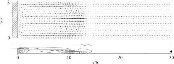
Figure 9. Three-dimensional flow structure of the critical eigenmode at Re= 750 and β = 0.9. Contours indicate the strength of the streamwise velocity component and vectors show the (v, w) flow pattern in each cross-sectional plane:x= 1.2, 6.2 and 12.2.
z h
ì
0
0 10 20 30
x/h
Figure 10.Sections of the critical three-dimensional eigenmode. Upper plot show (u, w) velocity vectors in the plane y=−0.65 (indicated by a triangle at the right of the lower plot). The lower plot containswvelocity contours (in the planez=λ/4) with solid and dashed contours indicating the sign ofw.
behind the step edge and at the downstream reattachment point (x1 '13.2). The
[image:17.595.149.443.394.502.2]secondary flow generated by the instability can best be described as a flat roll lying within the primary recirculation zone. This flow is qualitatively similar to the transient secondary flow sketched by Denham & Patrick (1974) following perturbations to the two-dimensional flow at Reynolds number 344. However, the spanwise wavelength of 6.9h is considerably smaller than that reported by Denham & Patrick (1974). We make further comparison with experiment in section §5.
Figure 11 shows the modes associated with the next three largest eigenvalues in the spectrum atRe= 750 andβ= 0.9 (see table 2 and figure 7). The next real eigenmode (corresponding to σ2 ' −0.013) plotted in figure 11(a) is localized to the secondary
separation region on the upper wall. The separation and reattachment points on the upper wall are located at x2 '10 and x3'25, respectively. This secondary mode is
z h
ì
0
0 10 20 30
x/h
(a)
(b)
(c)
z h
ì
0
0 10 20 30
z h
ì
0
0 10 20 30
Figure 11.Structure of the next three eigenmodes atRe= 750 andβ = 0.9: (a) real eigenmode corresponding to eigenvalue σ2; (b) and (c) real and imaginary parts of the complex eigenmode
corresponding to eigenvaluesσ3±iω3. In each case the upper plot show (u, w) velocity vectors in
they-plane indicated at the right of the lower plot. The lower plot containswvelocity contours in the planez=λ/4.
modes but are associated with quite different regions of the flow. The first complex mode is displayed in figure 11(b,c) in terms of its real and imaginary parts. The dynamics associated with this mode is a periodic oscillation between the two states. While it is principally associated with the primary recirculation region, this mode does extend into the upper recirculation region as well. The flow has a more complicated spatial structure with several ‘rolls’ within the primary recirculation region: the sign of the spanwise velocity component changes two (figure 11b) and three (figure 11c) times.
Finally, for completeness we show in figure 12 one of the channel modes whose eigenvalues are plotted in figure 7 (the one with right-most eigenvalue). As is evident from the spectrum, numerous similar modes are found in our computations. However, these modes are irrelevant to the linear instability of the step flow and we do not consider them further.
4.3. Two-dimensional stability
z h
ì
0
0 10 20 30
x/h
Figure 12.Structure of the channel eigenmode corresponding to the channel eigenvalue with largest real part. Only the real part of the complex eigenmode is plotted.
arises of when the flow becomes linearly unstable two-dimensionally. This has been a point of some controversy in previous computational studies of the two-dimensional flow (see Gresho et al. 1993). While this is not the focus of our study and our numerical methods have not been designed to study large Reynolds numbers for this flow, we have nevertheless continued the two-dimensional stability computations to
Re= 1500, twice the critical value for the onset of three-dimensional instability. The flow remains linearly stable to two-dimensional perturbations and moreover shows no evidence of any nearby two-dimensional bifurcation. Because accurate computations become very demanding at large Reynolds numbers and because there is no evidence that an instability is at hand, we cannot report a threshold for two-dimensional instability but only a lower bound for this threshold.
In figure 13 we plot, as a function of Reynolds number, the two leading eigenvalues from strictly two-dimensional stability computations, i.e. modes of the form
˜
u(x, y) = ( ˆu(x, y),vˆ(x, y),0), p˜(x, y) = ˆp(x, y). (4.1) Eigenvalues for all Reynolds numbers greater than 1050 have been computed with outflow length Lo = 55 and with polynomial orderN= 9. For lower Reynolds num-bers, shorter domains have been used consistent with convergence studies in §3.3. Recall (§3.1) that the two-dimensional base flows above Re= 800 are computed by time integration to a steady state. While this computational method is slow, it has the advantage here of confirming that all of the steady two-dimensional flows we have computed are globally stable with respect to two-dimensional perturbations.
The two eigenvalue branches approach one another at Re ≈ 1250. Generically, as the point of intersection is approached, the eigenvalues will either coalesce in a complex conjugate pair or will instead remain real and undergo avoided crossing. We find that the leading eigenvalues plotted in figure 13 remain real.
–3
400 800
Re
1200 1600 –2
–1
lo
g (–
r
)
Figure 13.Leading two-dimensional eigenvalues. The two branches (denoted by different symbols) remain real as they approach and recede from one another through the avoided crossing at Re≈1250.
5. Discussion
A detailed comparison between our linear stability calculations and either previous experimental work or direct numerical simulations is complicated by several factors. Among these are the existence of a strong convective instability within the core flow, the variety of geometries used in previous studies (expansion ratio, aspect ratio, sidewalls, no sidewalls), different upstream flow conditions, and so forth. Of these effects, the convective instability within the core flow is the most problematic as it renders the system particularly sensitive to upstream conditions, including free-stream noise and external perturbations. The flow may amplify selective components of these perturbations to produce apparent three-dimensionality and unsteadiness well before the onset of any absolute instability. The combined effects of these discrepancies mean that there is no single experiment or computation with which we can make a detailed comparison. In the following we compare our results with data available in the existing literature and try to indicate what further work might help clarify the nature of the absolute instability.
5.1. Comparison with previous work
We begin by comparing our results with the experimental work of Armaly et al. (1983) and the related computations by Williams & Baker (1997) in a system with a nominal expansion ratio of 2 and aspect ratioLz/h= 37. In both the experiments and computations the span of the channel terminated at a solid wall on both sides. These investigators found that below Re = 300 the flow is essentially spanwise invariant while above Re= 300 there is evidence of three-dimensionality in the flow. The value
Re= 300 does not necessarily indicate a critical point. Williams & Baker (1997) note that some deviation from two-dimensionality exists near the sidewalls of the channel below Re = 300, and neither study attempted to pinpoint the value ofRe at which significant three-dimensionality along the span first appeared in the system. Even the characterization of ‘significant’ is arbitrary.
both studies indicate that three-dimensionality is limited to the region within a few step heights of the sidewalls while the bulk flow remains largely spanwise-invariant at these low Reynolds numbers. This type of extrinsic effect is produced by the three-dimensional geometry of the laboratory setup, and it will surely depend on the aspect ratio of the system. It does not represent a fundamental instability of the nominally two-dimensional separated flow.
There is further computational evidence that the sidewalls play an important role. In the three-dimensional simulations of Kaiktsiset al. (1991) using spanwise-periodic boundary conditions, sustained three-dimensionality was first found at a much higher Reynolds number,Re'525, than was found in the numerical studies with sidewalls by Williams & Baker (1997). Interestingly, Kaiktsiset al. (1991) used a spanwise-periodic domain of length 2π, almost exactly the critical wavelengthλc= 6.9hdetermined by our analysis. However, even without sidewall effects the onset of three-dimensionality in the work of Kaiktsis et al. (1991) is still below Rec. There are two possible explanations for this.
The first is that the states observed by Kaiktsis et al. (1991) follow from am-plification of numerical noise due to poor resolution in the form of a convective instability. In later work, Kaiktsis et al. (1996) show this to be the source of the sustained two-dimensional dynamics observed by Kaiktsiset al. (1991) at Re= 600. Our computations are free from any such effects in that we determine only global absolute instability thresholds. However, we have performed preliminary nonlinear calculations of the three-dimensional flow, i.e. direct numerical simulations, that do confirm the existence of a strongly three-dimensional convective instability. These dynamics are poorly understood.
The other possible explanation for sustained three-dimensionality belowRecis that the instability is subcritical. From our linear computations we cannot know whether or not stable, nonlinear, three-dimensional states exist below the linear stability threshold. Whether or not this is the case, the simulation results of Kaiktsis et al. (1991, figures 11 and 24) indicate strong three-dimensionality primarily in the region downstream of the separation zone, and bear little qualitative resemblance to the critical eigenmode. Therefore it seems unlikely that their results provide any evidence of a subcritical bifurcation due to the absolute instability of the flow. This is an interesting point, but further computational work is required to assess whether or not the three-dimensional bifurcation is subcritical.
two peaks in the eigenvalue spectra in figure 6, and at lower Reynolds numbers the small-β peak actually corresponds to a larger eigenvalue, i.e. a slower decay rate. It is therefore possible that Denham & Patrick (1974) have observed evidence of these three-dimensional modes. Other researchers have also reported dynamics within the primary recirculation region, but it is not clear how to connect these flows to the eigenmode.
5.2. Instability mechanisms
Our stability calculations are unambiguous with regard to the critical Reynolds number, wavelength, and flow structure associated with the absolute instability. Here we address the question of why the flow amplifies this particular type of perturbation. One obvious a priori candidate is the Kelvin–Helmholtz instability of the shear layer emanating from the step edge. Although the Kelvin–Helmholtz instability is important at higher Reynolds number and as a source of amplification in the context of convective instability, it plays no role here because the three-dimensional instability is absolute. Furthermore, because of the relative thickness of the shear layer at these Reynolds numbers, and the stabilizing effect of the walls, it is difficult to excite any shear layer response in this parameter range.
Armaly et al. find that three-dimensionality first appears close to the Reynolds number at which the upper separation bubble forms. Ghia et al. (1989) postulate that once the secondary separation bubble forms, the main flow is subjected to a destabilizing concave curvature resulting in a three-dimensional, Taylor–G¨ortler-type instability. This is an interesting speculation. However, from our linear stability computations we can also rule this out. We find not only that the two-dimensional flow remains linearly stable long after the formation of the upper separation bubble, but also that when instability does set in, it is not of the form of streamwise vortices within the main flow as would be expected by this mechanism.
We argue that the essential mechanism is still centrifugal in nature but is associated with the closed streamlines in the primary recirculation zone near the solid boundaries. The basic inviscid condition for a centrifugal instability is Rayleigh’s criterion (e.g. Drazin & Reid 1981) and its generalization by Bayly (1988). Physically, in a flow with closed streamlines one expects instability to arise if there is an outward decrease in the magnitude of angular momentum. To investigate this, let η ≡ −∂|r×u|2/∂r,
wherer= (x−xc, y−yc) with (xc, yc) the centre about which the angular momentum is defined. We take this to be the point where the velocity vanishes, but in fact the results shown below depend only weakly on the choice of (xc, yc) for any reasonable choice. The flow is (inviscidly) centrifugally unstable where η >0.
Figure 14(a) shows the regions inside the primary recirculation zone where η is significantly positive for the two-dimensional flow at the critical Reynolds number. The regions where the magnitude of the angular momentum decreases significantly radially outwards are just behind the step face and just upstream of the re-attachment point. (All along the bottom wall and the step faceηis small and positive. For clarity we do not show regions whereηis less than 0.5% of the maximum value ofη= 0.13.) The regions shown in figure 14(a) are those for which the inviscid Rayleigh criterion predicts three-dimensional instability. Note that these are indeed the regions in which the magnitude of spanwise perturbation velocity is largest. See figure 14(b).
0 10
x/h
(a)
(b)
Figure 14. (a) Regions (black) where the magnitude of the angular momentum decreases away from the centre (marked with a cross) of the primary recirculation zone for the two-dimensional flow at Reynolds number 750. Specifically, the regions are shown whereηis greater than 0.5% of its maximum value. Also shown are representative streamlines. (b) Contours of the magnitude of the spanwise velocity componentwin the critical eigenmode. The separating streamline of the base flow is also shown.
of rotation, and the presence of the walls forces it to flow along the span to form the flat roll structure observed in the eigenmode. The spanwise length scale is not directly related to the step height but instead depends on the length of the separation bubble within which these three-dimensional eddies are generated.
The centrifugal mechanism is fundamentally three-dimensional in nature. This explains our finding that the backward-facing step flow does not become unstable two-dimensionally even at Reynolds numbers of twice the critical value for the onset of the three-dimensional instability. Some other mechanism would need to come into play at larger Reynolds numbers in order for this flow to become two-dimensionally unstable. For example, the upper separation bubble may become globally unstable (Hammond & Redekopp 1998; Alam & Sandham 2000). The flow will certainly become linearly unstable atRe= 2×5772 (e.g. Bayly et al. 1988) when flow in the downstream channel becomes unstable (the factor of 2 accounts for the difference between the Reynolds number used in this paper and the Reynolds number which applies to the downstream channel).
6. Conclusion
We have shown that the primary bifurcation of the steady, two-dimensional flow over a backward-facing step with a 2:1 expansion is a steady, three-dimensional instability. We have computed the critical Reynolds number and spanwise wavelength of the instability to high precision and findRec= 748 andλc= 6.9 in non-dimensional units based on the step height and the centreline velocity of the inflow. We have further determined the band of unstable wavenumbers for Reynolds numbers up to 1000. These data will be particularly useful in future numerical work as they allow the precise selection of appropriate spanwise domain lengths.
We have found that the critical eigenmode consists of a flat roll localized to the primary recirculation region located behind the step edge. Thus, at the linear level, the instability does not arise in either the secondary recirculation zone on the wall opposite the step or the core flow between the primary and secondary recirculation zones. From this we have been able to rule out a Taylor–G¨ortler-type instability of the main flow as the source of three-dimensionality in experiments, but have argued that centrifugal instability is responsible for generating secondary flow with the separation zone.
a lower limit for such a bifurcation of Re= 1500, considerably above the critical Reynolds number for three-dimensional instability. This establishes the fundamental role of three-dimensionality for separated flows similar to this one.
Following on from this work and the work of Kaiktsis et al. (1996), future studies should be conducted to examine three-dimensional convective instabilities of the backward-facing step. In the same way it would also be important to extend this work to nonlinear stability computations and determine whether the bifurcations are supercritical or subcritical.
We thank G. Brown and P. Marcus for many useful discussions on the topic of centrifugal instability. M. G. M. G. acknowledges support from the EPSRC, UK and the FCT, Portugal, and the hospitality of the IMA, University of Minnesota, where part of this research was carried out. R. H. H. acknowledges support from the NSF.
REFERENCES
Adams, E. W. & Johnston, J. P.1988 Effects of the separating shear-layer on the reattachment flow structure part 2: reattachment length and wall shear-stress.Exps. Fluids6, 493–499.
Akselvoll, K. & Moin, P. 1993 Large eddy simulation of a backward-facing step flow. In
En-gineering Turbulence Modeling and Experiments 2 (ed. W. Rodi & F. Martelli), pp. 303–313.
Elsevier.
Alam, M. & Sandham, N. D.2000 Direct numerical simulation of ‘short’ laminar separation bubbles with turbulent reattachment.J. Fluid Mech.410, 1–28.
Armaly, B. F., Durst, F., Pereira, J. C. F. & Sch¨onung, B.1983 Experimental and theoretical investigation of backward-facing step flow.J. Fluid Mech.127, 473–496.
Avva, R. K.1988 Computation of the turbulent flow over a backward-facing step using the zonal modeling approach. PhD thesis, Stanford University.
Barkley, D. & Henderson, R. D.1996 Three-dimensional Floquet stability analysis of the wake of a circular cylinder.J. Fluid Mech.322, 215–241.
Barkley, D. & Tuckerman, L. S.1999 Stability analysis of perturbed plane Couette flow.Phys.
Fluids A11, 1187–1195.
Bayly, B. J.1988 Three-dimensional centrifugal-type instabilities in inviscid two-dimensional flows.
Phys. Fluids 31, 56–64.
Bayly, B. J., Orszag, S. A. & Herbert, T.1988 Instability mechanisms in shear-flow transition.
Annu. Rev. Fluid Mech.20, 359–391.
Bernardi, C., Maday, Y. & Patera, A. T. 1992 A new nonconforming approach to domain decomposition: the mortar element method. In Nonlinear Partial Differential Equations and
their Application(ed. H. Brezis & J. L. Lyons). Pitman and Wiley.
Butler, K. M. & Farrell, B. F.1993 Optimal perturbations and streak spacing in wall-bounded turbulent shear-flow.Phys. Fluids A5, 774–777.
Denham, M. K. & Patrick, M. A.1974 Laminar flow over a downstream-facing step in a two-dimensional flow channel.Trans. Inst. Chem. Engrs 52, 361–367.
Drazin, P. G. & Reid, W. H.1981Hydrodynamic Stability. Cambridge University Press.
Edwards, W. S., Tuckerman, L. S., Friesner, R. A. & Sorensen, D. C.1994 Krylov methods for the incompressible Navier–Stokes equations.J. Comput. Phys.110, 82–102.
Fortin, A., Jardak, M., Gervais, J. J. & Pierre, R.1997 Localization of Hopf bifurcations in fluid flow problems.Intl J. Numer. Meth. Fluids24, 1185–1210.
Gartling, D. K.1990 A test problem for outflow boundary-conditions – flow over a backward-facing step.Intl J. Numer. Meth. Fluids 11, 953–967.
Ghia, K. N., Osswald, G. A. & Ghia, U. 1989 Analysis of incompressible massively separated viscous flows using unsteady Navier–Stokes equations. Intl J. Numer. Meth. Fluids 9, 1025– 1050.
Goldstein, R. J., Eriksen, V. L., Olson, R. M. & Eckert, E. R. G. 1970 Laminar separation, reattachment, and transition of the flow over a downstream-facing step. Trans. ASME D:
Gresho, P. M., Gartling, D. K., Torczynski, J. R., Cliffe, K. A., Winters, K. H., Garratt, T. J., Spence, A. & Goodrich, J. W. 1993 Is the steady viscous incompressible two-dimensional flow over a backward-facing step atRe= 800 stable?Intl J. Numer. Meth. Fluids 17, 501–541.
Hamilton, J. M., Kim, J. & Waleffe, F.1995 Regeneration mechanisms of near-wall turbulence structures.J. Fluid Mech.287, 317–348.
Hammond, D. A. & Redekopp, L. G. 1998 Local and global instability properties of separation bubbles.Eur. J. Mech.B/Fluids 17, 145–164.
Henderson, R. D.1994 Unstructured spectral element methods: parallel algorithms and simulations. PhD thesis, Princeton University.
Henderson, R. D. & Karniadakis, G. E.1995 Unstructured spectral element methods for simulation of turbulent flows.J. Comput. Phys.122, 191–217.
Huerre, P. & Monkewitz, P. A.1990 Local and global instabilities in spatially developing flows.
Annu. Rev. Fluid Mech.22, 473–537.
Kaiktsis, L., Karniadakis, G. E. & Orszag, S. A. 1991 Onset of three-dimensionality, equilibria, and early transition in flow over a backward-facing step.J. Fluid Mech.231, 501–528.
Kaiktsis, L., Karniadakis, G. E. & Orszag, S. A. 1996 Unsteadiness and convective instabilities in two-dimensional flow over a backward-facing step.J. Fluid Mech.321, 157–187.
Karniadakis, G. E., Israeli, M. & Orszag, S. A. 1991 High-order splitting methods for the incompressible Navier–Stokes equations.J. Comput. Phys.97, 414–443.
Le, H., Moin, P. & Kim, J.1997 Direct numerical simulation of turbulent flow over a backward-facing step.J. Fluid Mech.330, 349–374.
Mamun, C. K. & Tuckerman, L. S. 1995 Asymmetry and Hopf bifurcation in spherical Couette flow.Phys. Fluids 7, 80–91.
Patera, A. T. 1984 A spectral element method for fluid dynamics: laminar flow in a channel expansion.J. Comput. Phys.54, 468–488.
Saad, Y. & Schultz, M. H. 1986 Gmres – a generalized minimal residual algorithm for solving nonsymmetric linear-systems.SIAM J. Sci. Statist. Comput.7, 856–869.
Schatz, M. F., Barkley, D. & Swinney, H. L.1995 Instabilities in spatially periodic channel flow.
Phys. Fluids 7, 344–358.