Hierarchical Directed Acyclic Graph Kernel:
Methods for Structured Natural Language Data
Jun Suzuki, Tsutomu Hirao, Yutaka Sasaki, and Eisaku Maeda
NTT Communication Science Laboratories, NTT Corp. 2-4 Hikaridai, Seika-cho, Soraku-gun, Kyoto, 619-0237 Japan
jun, hirao, sasaki, maeda @cslab.kecl.ntt.co.jp
Abstract
This paper proposes the “Hierarchical Di-rected Acyclic Graph (HDAG) Kernel” for structured natural language data. The HDAG Kernel directly accepts several lev-els of both chunks and their relations, and then efficiently computes the weighed sum of the number of common attribute sequences of the HDAGs. We applied the proposed method to question classifica-tion and sentence alignment tasks to eval-uate its performance as a similarity mea-sure and a kernel function. The results of the experiments demonstrate that the HDAG Kernel is superior to other kernel functions and baseline methods.
1 Introduction
As it has become easy to get structured corpora such as annotated texts, many researchers have applied statistical and machine learning techniques to NLP tasks, thus the accuracies of basic NLP tools, such as POS taggers, NP chunkers, named entities tag-gers and dependency analyzers, have been improved to the point that they can realize practical applica-tions in NLP.
The motivation of this paper is to identify and use richer information within texts that will improve the performance of NLP applications; this is in con-trast to using feature vectors constructed by a bag-of-words (Salton et al., 1975).
We now are focusing on the methods that use nu-merical feature vectors to represent the features of
natural language data. In this case, since the orig-inal natural language data is symbolic, researchers convert the symbolic data into numeric data. This process, feature extraction, is ad-hoc in nature and differs with each NLP task; there has been no neat formulation for generating feature vectors from the semantic and grammatical structures inside texts.
Kernel methods (Vapnik, 1995; Cristianini and Shawe-Taylor, 2000) suitable for NLP have recently been devised. Convolution Kernels (Haussler, 1999) demonstrate how to build kernels over discrete struc-tures such as strings, trees, and graphs. One of the most remarkable properties of this kernel method-ology is that it retains the original representation of objects and algorithms manipulate the objects simply by computing kernel functions from the in-ner products between pairs of objects. This means that we do not have to map texts to the feature vectors by explicitly representing them, as long as an efficient calculation for the inner products be-tween a pair of texts is defined. The kernel method is widely adopted in Machine Learning methods, such as the Support Vector Machine (SVM) (Vap-nik, 1995). In addition, kernel function
has been described as a similarity function that satisfies certain properties (Cristianini and Shawe-Taylor, 2000). The similarity measure between texts is one of the most important factors for some tasks in the application areas of NLP such as Machine Trans-lation, Text Categorization, Information Retrieval, and Question Answering.
cal-culate the similarity with regard to these structures at practical cost and time. The HDAG Kernel can be widely applied to learning, clustering and similarity measures in NLP tasks.
The following sections define the HDAG Kernel and introduce an algorithm that implements it. The results of applying the HDAG Kernel to the tasks of question classification and sentence alignment are then discussed.
2 Convolution Kernels
Convolution Kernels were proposed as a concept of kernels for a discrete structure. This framework de-fines a kernel function between input objects by ap-plying convolution “sub-kernels” that are the kernels for the decompositions (parts) of the objects.
Let be a positive integer and
be nonempty, separable metric spaces. This paper focuses on the special case that are
countable sets. We start with as a composite structure and
as its “parts”, where ! "#$ . % is defined as a relation on the set '&
(((
& )& such that%*+, is true if are the
“parts” of .
/ is defined as
/,13254 %67,89
Suppose :; , be the parts of with < , and = be the parts of with =>? . Then, the similarity @/
be-tween and is defined as the following
general-ized convolution:
A$BDCFEHGJILK
MONOPRQFSTVUW XONOPYQFST[ZW
\
]_^a`
A
]
BDC
]
EbG
]
I7c
(1)
We note that Convolution Kernels are abstract con-cepts, and that instances of them are determined by the definition of sub-kernel # 9/d 9 J Y . The Tree Kernel (Collins and Duffy, 2001) and String Subse-quence Kernel (SSK) (Lodhi et al., 2002), developed in the NLP field, are examples of Convolution Ker-nels instances.
An explicit definition of both the Tree Kernel and SSK@/ is written as:
A$BDCFEeG9IfKgihjBDCFIlkmh9BDGJI7noK;p
q
^a`
h
q
BDCoIokrh
q
BDG9I7c
(2)
Conceptually, we enumerate all sub-structures oc-curring in and , where s represents the
to-tal number of possible sub-structures in the ob-jects. t , the feature mapping from the sample
space to the feature space, is given by td>
t /tduv
In the case of the Tree Kernel, and be trees.
The Tree Kernel computes the number of common subtrees in two trees and . tdw_ is defined as
the number of occurrences of the x ’th enumerated
subtree in tree .
In the case of SSK, input objects and are
string sequences, and the kernel function computes the sum of the occurrences ofx ’th common
subse-quencet w / weighted according to the length of the
subsequence. These two kernels make polynomial-time calculations, based on efficient recursive cal-culation, possible, see equation (1). Our proposed method uses the framework of Convolution Kernels.
3 HDAG Kernel
3.1 Definition of HDAG
This paper defines HDAG as a Directed Acyclic Graph (DAG) with hierarchical structures. That is, certain nodes contain DAGs within themselves.
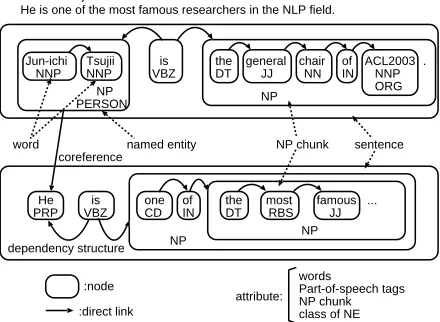
In basic NLP tasks, chunking and parsing are used to analyze the text semantically or grammatically. There are several levels of chunks, such as phrases, named entities and sentences, and these are bound by relation structures, such as dependency structure, anaphora, and coreference. HDAG is designed to enable the representation of all of these structures inside texts, hierarchical structures for chunks and DAG structures for the relations of chunks. We be-lieve this richer representation is extremely useful to improve the performance of similarity measure be-tween texts, moreover, learning and clustering tasks in the application areas of NLP.
Figure 1 shows an example of the text structures that can be handled by HDAG. Figure 2 contains simple examples of HDAG that elucidate the calcu-lation of similarity.
Word-is of
PERSON
NNP NNP VBZ
word named entity NP chunk
dependency structure
sentence coreference
.
... Jun-ichi Tsujii the general chair ACL2003
He is one of the most famous
Junichi Tsujii is the Gereral Chair of ACL2003. He is one of the most famous researchers in the NLP field.
:node
:direct link
DT JJ NN IN NNP
NP NP
PRP VBZ CD IN DT RBS JJ
NP NP
ORG
attribute: words
[image:3.612.76.296.79.240.2]Part-of-speech tags NP chunk class of NE
Figure 1: Example of the text structures handled by HDAG
p1 p2 p3 p4 p5 G1
G2
q1 q3 q4 q6
N
V a
b d a
c
N e b
c
a d
q8
q2 q5 q7
p6 p7
NP
NP
Figure 2: Examples of HDAG structure
Net, and class of the named entity.
3.2 Definition of HDAG Kernel
First of all, we define the set of nodes in HDAGs
y
and y{z
as| and} , respectively,~ and
repre-sent nodes in the graph that are defined as 2~,~ w |x J|8 and2JY}#3a}8 ,
respectively. We use the expression~ 6 ~J ~f
to represent the path from~ to~ through~ .
We define “attribute sequence” as a sequence of attributes extracted from nodes included in a sub-path. The attribute sequence is expressed as ‘A-B’ or ‘A-(C-B)’ where ( ) represents a chunk. As a ba-sic example of the extraction of attribute sequences from a sub-path,
z
in Figure 2 contains the
four attribute sequences ‘e-b’, ‘e-V’, b’ and ‘N-V’, which are the combinations of all attributes in
z
and . Section 3.3 explains in detail the method of
extracting attribute sequences from sub-paths. Next, we define “terminated nodes” as those that do not contain any graph, such as ~
z
, ~l ;
“non-terminated nodes” are those that do, such as , .
Since HDAGs treat not only exact matching of sub-structures but also approximate matching, we allow node skips according to decay factor ! $J when extracting attribute sequences from the
sub-paths. This framework makes similarity evalua-tion robust; the similar sub-structures can be eval-uated in the value of similarity, in contrast to ex-act matching that never evaluate the similar sub-structure. Next, we define parameter ( JJ) as the number of attributes combined in the
attribute sequence. When calculating similarity, we consider only combination lengths of up to .
Given the above discussion, the feature vector of HDAG is written astd
y
' t
y
_tdu@
y
,
where t represents the explicit feature mapping of
HDAG ands represents the number of all possible attribute combinations. The value of t w
y
is the
number of occurrences of thex ’th attribute sequence
in HDAG
y
; each attribute sequence is weighted ac-cording to the node skip. The similarity between HDAGs, which is the definition of the HDAG Ker-nel, follows equation (2) where input objects and
are
y
and y{z
, respectively. According to this ap-proach, the HDAG Kernel calculates the inner prod-uct of the common attribute sequences weighted ac-cording to their node skips and the occurrence be-tween the two HDAGs,y
and y z
.
We note that, in general, if the dimension of the feature space becomes very high or approaches in-finity, it becomes computationally infeasible to gen-erate feature vectortd
y
explicitly. To improve the
reader’s understanding of what the HDAG Kernel calculates, before we introduce our efficient calcu-lation method, the next section details the attribute sequences that become elements of the feature vec-tor if the calculation is explicit.
3.3 Attribute Sequences: The Elements of the Feature Vector
We describe the details of the attribute sequences that are elements of the feature vector of the HDAG Kernel usingy
and y z
in Figure 2.
The framework of node skip
We denote the explicit representation of a node skip by ” ”. The attribute sequences in the sub-path
Table 1: Attribute sequences and the values of nodes
~! and
`
sub-path a. seq. val.
¡
K¢
`
NP 1
j£
a-¤ ¥
£
N-¤ ¥
Y¦
c-¤ ¥
§
¤ -b ¨¥
¡
K
¨
j£ª© §
a-b 1
j£ª© §
N-b 1
¦ © §
c-b 1
« §
sub-path a. seq. val.
¡
K¢ « §
NP 1
«¬
(¤ -¤ )-a ¥
£
«
(c-¤ )-¤ ¥
£
«
(¤ -d)-¤ ¥
£
¡
K
¨
«
(c-d)-¤ ¥ « ©®«¬
(c-¤ )-a ¥ « ©®«¬
(¤ -d)-a ¥
¡
K¯ «O°©®« ¬
(c-d)-c 1
non-terminated node is the same as skipping all the graphs inside the non-terminated node. We intro-duce decay functions±²~f ,³°²o/~f and ´'²/~f; all
are based on decay factor . ±.²a~f represents the
cost of node skip~ . For example, ± ² /~dµJ
z
represents the cost of node skip~
z
¶ and that
of~ ~J ; ±²/~
z
µ is the cost of just node
skip~
z
. ³²/~f represents the sum of the multiplied
cost of the node skips of all of the nodes that have a path to~ ,³²o/~j1 9 that is the sum cost of both
~
z
and~ that have a path to~ , ³²o/~ "·9o¸Y . ´ ² /~f represents the sum of the multiplied cost of
the node skips of all the nodes that ~ has a path
to. ´¹²!/~
z
@º represents the cost of node skip ~l where~
z
has a path to~F .
Attribute sequences for non-terminated nodes
We define the attributes of the non-terminated node as the combinations of all attribute sequences including the node skip. Table 1 shows the attribute sequences and values of~
and .
Details of the elements in the feature vector
The elements of the feature vector are not consid-ered in any of the node skips. This means that
‘A- -B-C’ is the same element as ‘A-B-C’, and ‘A- -
-B-C’ and ‘A- -B- -C’ are also the same element as
‘A-B-C’. Considering the hierarchical structure, it is natural to assume that ‘(N- )-(d)-a’ and ‘(N- )-((
-d)-a)’ are different elements. However, in the frame-work of the node skip and the attributes of the non-terminated node, ‘(N- )-( )-a’ and ‘(N- )-(( - )-a)’
[image:4.612.326.527.97.320.2]are treated as the same element. This framework
Table 2: Similarity values of and in Figure 2
»
`
»
£
att. seq. value att. seq. value
¡
K¢
NP 1 NP 1 1
N 1 N 1 1
a 2 a 1 2
b 1 b 1 1
c 1 c 1 1
d 1 d 1 1
¡
K
¨
(N-¤ )-(¤ )-a ¥
£
(N-¤ )-((¤ -¤ )-a) ¥
¦
¥
¬
N-b 1 N-b 1 1
(N-¤ )-(d) ¥ (N-¤ )-((¤ -d)-¤ ) ¥
¦
¥
§
(¤ -b)-(¤ )-a ¨¥
£
(¤ -b)-((¤ -¤ )-a) ¥
¦
¨¥
¬
(¤ -b)-(d) ¨¥ (¤ -b)-((¤ -d)-¤ ) ¥
¦
¨¥
§
(c-¤ )-(¤ )-a ¥
£
((c-¤ )-a) ¥ ¥
¦
(c-¤ )-(d) ¥ c-d 1 ¥
(d)-a 1 (c-¤ )-a ¥ ¥
¡
K¯
(N-b)-(¤ )-a ¥ (N-b)-((¤ -¤ )-a) ¥
£
¥
¦
(N-b)-(d) 1 (N-b)-((¤ -d)-¤ ) ¥
£
¥
£
achieves approximate matching of the structure au-tomatically, The HDAG Kernel judges all pairs of attributes in each attribute sequence that are inside or outside the same chunk. If all pairs of attributes in the attribute sequences are in the same condition, inside or outside the chunk, then the attribute se-quences judge as the same element.
Table 2 shows the similarity, the values of
"¼ ½!¾
y
y
z
, when the feature vectors are
ex-plicitly represented. We only show the common ele-ments of each feature vector that appear in both
y
andy z
, since the number of elements that appear in onlyy
or y{z
becomes very large.
Note that, as shown in Table 2, the attribute se-quences of the non-terminated node itself are not addressed by the features of the graph. This is due to the use of the hierarchical structure; the attribute sequences of the non-terminated node come from the combination of the attributes in the terminated nodes. In the case of ¶9 , attribute sequence ‘N- ’
comes from ‘N’ in¶
z
. If we treat both ‘N- ’ in~°
and ‘N’ in~
z
, we evaluate the attribute sequence ‘N’ in~
z
twice. That is why the similarity value in Ta-ble 2 does not contain ‘c- ’ in~ and ‘(c- )- ’ in ,
[image:4.612.84.288.114.258.2]3.4 Calculation
First, we determine ¿FÀ6 ¶ ÁO , which returns the
sum of the common attribute sequences of theÂ
-combination of attributes between nodes~ and .
ÃRÄÅB7ÆEbÇILK Ã°È Ä B E « IaÉÊËÌ7B E « I7E if Í K#¢ Ã È Ä B E « I7E otherwise (3) Ã È Ä B E « IfK Î E if Ï ¡ B IfKÑÐ and Ï ¡ B « IfKÑÐ Ò7N qÔÓ TVÕ+W
Ö× B7ÆIlk7Ø × B7ÆIlk7ÊËÌ7B7ÆE
« I7E if Ï ¡ B IÙK"Ð and Ï ¡ B « IdK"Ð Ú N qHÓ TVÕ7W
Ö× BDÇIlk_Ø × BDÇIlk_ÊËÌ7B
EbÇI7E if Ï ¡ B IfK"Ð and Ï ¡ B « IÙK"Ð Ò7N qÔÓ TÛW Ú N qHÓ TVÕ7W
ØÜ×B7ÆIak7Ø'×BDÇIlk_Ý Ä B7ÆEbÇI/E
otherwise
(4)
Þdßaà
/~fj returns the number of common attributes
of nodes ~ and , not including the attributes of
nodes inside~ and . We define functionx+Å~f as
re-turning a set of nodes inside a non-terminated node
~ . x+Å~fáµâ means node~ is a terminated node.
For example,x+Å~!m2~
z
~ ~ 8 andx+Å~
z
,â .
We define functions ã{À.~f9, ã¹ä
À
/~fj and ã ää
À
/~fj to calculate¿fÀ/~f9 .
ݹÄB E « IfK#ÃRÄÅB E « IaÉ Äå ` æ ^` Ý È æ B E « IakOÃRÄå æ B E « I (5) Ý È Ä B E « IfK Ú Nç_è/éêTVÕ+W
ë × BêÇIlk7Ý
È Ä B EbÇIJÉÝ ÈÈ Ä B EbÇI (6) Ý ÈÈ Ä B E « ILK Ò7Nç_è/éêTÛW ë*×BiÆIlk7Ý ÈÈ Ä B7ÆE « IaÉ6Ý Ä B7ÆE « I (7)
The boundary conditions are
ݹÄB
E
«
IìK Ö× B
Iok Ö× B
« IakrÃYÄÅB E « I7E if Í K#¢ (8) Ý È Ä B E «
IìK Î E
if ímî Ì7B « ILKÑÐ (9) Ý ÈÈ Ä B E «
IìK Î E
if ímî Ì7B ILKÑÐ9c (10) FunctionïFð à
~f returns the set of nodes that have
direct links to node~ . ïFð
à
/~f1ñâ means no nodes
have direct links to ¶ . ïFð
à /~!jò 2~ z ~j8 and ïFð à ~ªm,â .
Next, we define @~f9 as representing the sum
of the common attribute sequences that are theÂ
-combinations of attributes extracted from the sub-paths whose sinks are~ and , respectively.
A.Ä,B E « ILK ÊËÌ7B E « I7E if Í K¢ Äå ` æ ^a`Ló È æ B E « Ilkà Äå æ B E « IE otherwise (11)
Functions ôÀ/~f9, ô
ä
À
/~fj and ô ää
À
~f9 ,
needed for the recursive calculation of À ~f9 , are
written in the same form asã'À"/~fj ,ã
ä
À
/~fj and ã ää
À
/~fj respectively, except for the boundary
con-dition ofô À /~fj , which is written as:
ó
Ä B
E
«
IìK Ã Ä B
E « I7E if Í K¢c (12)
Finally, an efficient similarity calculation formula is written as Aõ \öl÷ B» ` E » £ ILK Ó Ä ^` ÛmNOø Õ_NOù A.Ä,B E « I7c (13)
According to equation (13), given the recursive definition of $À./~fj, the similarity between two
HDAGs can be calculated inú/*|e} time 1.
3.5 Efficient Calculation Method
We will now elucidate an efficient processing algo-rithm. First, as a pre-process, the nodes are sorted under the following condition: all nodes that have a path to the focused node and are in the graph in-side the focused node should be set before the fo-cused node. We can get at least one set of ordered nodes since we are treating an HDAG. In the case of
y
, we can get ûÔ~
z
, ~J , ~J ,~ ,~ ,~lü ,~!ý . We
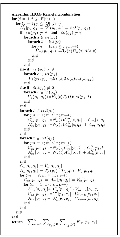
can rewrite the recursive calculation formula in “for loops”, if we follow the sorted order. Figure 3 shows the algorithm of the HDAG kernel. Dynamic pro-gramming technique is used to compute the HDAG Kernel very efficiently because when following the sorted order, the values that are needed to calculate the focused pair of nodes are already calculated in the previous calculation. We can calculate the table by following the order of the nodes from left to right and top to bottom.
We normalize the computed kernels before their use within the algorithms. The normalization cor-responds to the standard unit norm normalization of
1
We can easily rewrite the equation to calculate all combi-nations of attributes, but the order of calculation time becomes
þ
Biÿ'ÿVÿÅÿ[I
Algorithm HDAG Kernel n combination
for i++
for ++
S !#"%$'& ( S )*!+"$ ,-/./0 1!+"$
if +23 5476 and +2" $89476
foreach:;<+23
foreach=>;?+2" $8
for@ @AB23C@ ++ (,D !#" $'+=EF):GHEFI=+HJK: !=+
end end end
else if 2 9476
foreach:;<+23
(
S
G!C"$ +=E
F
:*HL
F
:GH-M./0: !+"$
end
else if 2"$5476
foreach=>;?+23
"ON
(JS !C"$8+=EFP=+HLF/=+H-M./0 !=+
end end
foreach:;?QR108 +
for@ S%@TB2@ ++ UWVV
D
!C"$8&+=
X
F
:G UWVV
D
:
!C"$'&MY
U
D
:
!C"$8&
J
VV
D
!C"$&+=XKFI:*HJ VV
D
: !#" $&MY JZD : !C"$&
end end
foreach=[;\Q%R0" $1
for@ S%@TB2@ ++ UWV
D
!C"$&+=XKF)=+ UWV
D
!=&MY U5VV
D
!=&
J
V
D
*!C"$8&+=X F =+HJ
V
D
/!=&Y J VV
D
*!=&
end end
U
S !+" $& (jS !C"$&
JªS !+" $& ]L^FI `_'LaFI"$*3_G(lS !C"$&
for@b7cP@AB23C@ ++
U
D !C"$& JZD !C"$& (D !C"$&
for.5 .edf@f'. ++
D !C"$&+= U V
g
!C"$& _1(,DaQ
g
!C" $&
U
D !C"$8&+= U V
g !C"$8& _1( DaQ
g
/!C"$8& JWD !C"$&+=J
V
g !C" $& _'(,DaQ
g
!C"$&
end end end end
return h
D3ioS j +k,l
N
$*k,m
[image:6.612.82.292.66.478.2]
D\ *!C"%$8&
Figure 3: Algorithm of the HDAG Kernel
examples in the feature space corresponding to the kernel space (Lodhi et al., 2002).
n
AáBDCFEbGJIFK
A$BDCFEeG9I
ABêCEDCFIak7A$BDGlEDGJI (14)
4 Experiments
We evaluated the performance of the proposed method in an actual application of NLP; the data set is written in Japanese.
We compared HDAG and DAG (the latter had no hierarchy structure) to the String Subsequence Ker-nel (SSK) for word sequence, Dependency Structure
p1 p2
p5 p4
p3 p6 p7
George Bush purchased a small interest in which baseball team ? NNP NNP VBD DT JJ NN IN WDT NN NN .
PERSON NP
NP PP NP
Question: George Bush purchased a small interest in which baseball team ?
p8 p9
p11 p10
p12 p13 p14
p1 p4 p5 p6 p7
George Bush purchased a small interest in which baseball team ? VBD DT JJ NN IN WDT NN NN . PERSON
p8 p9 p10 (a) Hierarchical and Dependency Structure
(b) Dependency Structure p2 p3
(c) Word Order
p1 p4 p5 p6 p7
George Bush purchased a small interest in which baseball team ? VBD DT JJ NN IN WDT NN NN . PERSON
[image:6.612.316.543.83.223.2]p8 p9 p10 p2 p3
Figure 4: Examples of Input Object Structure: (a) HDAG, (b) DAG and DSK’, (c) SSK’
Kernel (DSK) (Collins and Duffy, 2001) (a special case of the Tree Kernel), and Cosine measure for feature vectors consisting of the occurrence of at-tributes (BOA), and the same as BOA, but only the attributes of noun and unknown word (BOA’)were used.
We expanded SSK and DSK to improve the total performance of the experiments. We denote them as SSK’ and DSK’ respectively. The original SSK treats only exact string combinations based on
pa-rameter . We consider string combinations of up to for SSK’. The original DSK was specifically
con-structed for parse tree use. We expanded it to be able to treat the combinations of nodes and the free
or-der of child node matching.
Figure 4 shows some input objects for each eval-uated kernel, (a) for HDAG, (b) for DAG and DSK’, and (c) for SSK’. Note, though DAG and DSK’ treat the same input objects, their kernel calculation methods differ as do the return values.
We used the words and semantic information of “Goi-taikei” (Ikehara et al., 1997), which is similar to WordNet in English, as the attributes of the node. The chunks and their relations in the texts were an-alyzed by cabocha (Kudo and Matsumoto, 2002), and named entities were analyzed by the method of (Isozaki and Kazawa, 2002).
We tested each -combination case with changing
parameter from 0.1 through 0.9 in the step of 0.1.
Table 3: Results of the performance as a similarity measure for question classification
¡
1 2 3 4 5 6
HDAG - .580 .583 .580 .579 .573
DAG - .577 .578 .573 .573 .563
DSK’ - .547 .469 .441 .436 .436
SSK’ - .568 .572 .570 .562 .548
BOA .556
BOA’ .555
4.1 Performance as a Similarity Measure
Question Classification
We used the 1011 questions of NTCIR-QAC1 2 and the 2000 questions of CRL-QA data 3 We
as-signed them into 148 question types based on the CRL-QA data.
We evaluated classification performance in the following step. First, we extracted one question from the data. Second, we calculated the similar-ity between the extracted question and all the other questions. Third, we ranked the questions in order of descending similarity. Finally, we evaluated perfor-mance as a similarity measure by Mean Reciprocal Rank (MRR) (Voorhees and Tice, 1999) based on the question type of the ranked questions.
Table 3 shows the results of this experiment.
Sentence Alignment
The data set (Hirao et al., 2003) taken from the “Mainichi Shinbun”, was formed into abstract sen-tences and manually aligned to sensen-tences in the “Yomiuri Shinbun” according to the meaning of sen-tence (did they say the same thing).
This experiment was prosecuted as follows. First, we extracted one abstract sentence from the “Mainichi Shinbun” data-set. Second, we calculated the similarity between the extracted sentence and the sentences in the “Yomiuri Shinbun” data-set. Third, we ranked the sentences in the “Yomiuri Shinbun” in descending order based on the calculated similar-ity values. Finally, we evaluated performance as a similarity measure using the MRR measure.
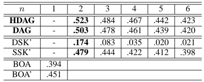
Table 4 shows the results of this experiment.
2
http://www.nlp.cs.ritsumei.ac.jp/qac/
3
http://www.cs.nyu.edu/˜sekine/PROJECT/CRLQA/
Table 4: Results of the performance as a similarity measure for sentence alignment
¡
1 2 3 4 5 6
HDAG - .523 .484 .467 .442 .423
DAG - .503 .478 .461 .439 .420
DSK’ - .174 .083 .035 .020 .021
SSK’ - .479 .444 .422 .412 .398
BOA .394
BOA’ .451
Table 5: Results of question classification by SVM with comparison kernel functions
¡
1 2 3 4 5 6
HDAG - .862 .865 .866 .864 .865
DAG - .862 .862 .847 .818 .751
DSK’ - .731 .595 .473 .412 .390
SSK’ - .850 .847 .825 .777 .725
BOA+poly .810 .823 .800 .753 .692 .625
BOA’+poly .807 .807 .742 .666 .558 .468
4.2 Performance as a Kernel Function
Question Classification
The comparison methods were evaluated the per-formance as a kernel function in the machine learn-ing approach of the Question Classification. We chose SVM as a kernel-based learning algorithm that produces state-of-the-art performance in several NLP tasks.
We used the same data set as used in the previous experiments with the following difference: if a ques-tion type had fewer than ten quesques-tions, we moved the entries into the upper question type as defined in CRL-QA data to provide enough training sam-ples for each question type. We used one-vs-rest as the multi-class classification method and found a highest scoring question type. In the case of BOA and BOA’, we used the polynomial kernel (Vapnik, 1995) to consider the attribute combinations.
Table 5 shows the average accuracy of each ques-tion as evaluated by 5-fold cross validaques-tion.
5 Discussion
[image:7.612.321.531.109.194.2]Ques-tion Type, which reflects the intenQues-tion of the ques-tion. The Sentence Alignment task evaluates which sentence is the most semantically similar to a given sentence.
The HDAG Kernel showed the best performance in the experiments as a similarity measure and as a kernel of the learning algorithm. This proves the usefulness of the HDAG Kernel in determining the similarity measure of texts and in providing an SVM kernel for resolving classification problems in NLP tasks. These results indicate that our approach, in-corporating richer structures within texts, is well suited to the tasks that require evaluation of the se-mantical similarity between texts. The potential use of the HDAG Kernel is very wider in NLP tasks, and we believe it will be adopted in other practical NLP applications such as Text Categorization and Ques-tion Answering.
Our experiments indicate that the optimal param-eters of combination number and decay factor
depend the task at hand. They can be determined by experiments.
The original DSK requires exact matching of the tree structure, even when expanded (DSK’) for flex-ible matching. This is why DSK’ showed the worst performance. Moreover, in Sentence Alignment task, paraphrasing or different expressions with the same meaning is common, and the structures of the parse tree widely differ in general. Unlike DSK’, SSK’ and HDAG Kernel offer approximate match-ing which produces better performance.
The structure of HDAG approaches that of DAG, if we do not consider the hierarchical structure. In addition, the structure of sequences (strings) is en-tirely included in that of DAG. Thus, the framework of the HDAG Kernel covers DAG Kernel and SSK.
6 Conclusion
This paper proposed the HDAG Kernel, which can reflect the richer information present within texts. Our proposed method is a very generalized frame-work for handling the structure inside a text.
We evaluated the performance of the HDAG Ker-nel both as a similarity measure and as a kerKer-nel func-tion. Our experiments showed that HDAG Kernel offers better performance than SSK, DSK, and the baseline method of the Cosine measure for feature
vectors, because HDAG Kernel better utilizes the richer structure present within texts.
References
M. Collins and N. Duffy. 2001. Parsing with a Single Neuron: Convolution Kernels for Natural Language Problems. In Technical Report UCS-CRL-01-10. UC Santa Cruz.
N. Cristianini and J. Shawe-Taylor. 2000. An In-troduction to Support Vector Machines and Other Kernel-based Learning Methods. Cambridge
Univer-sity Press.
D. Haussler. 1999. Convolution Kernels on Discrete Structures. In Technical Report UCS-CRL-99-10. UC Santa Cruz.
T. Hirao, H. Kazawa, H. Isozaki, E. Maeda, and Y. Mat-sumoto. 2003. Machine Learning Approach to Multi-Document Summarization. Journal of Natural
Lan-guage Processing, 10(1):81–108. (in Japanese).
S. Ikehara, M. Miyazaki, S. Shirai, A. Yokoo, H. Nakaiwa, K. Ogura, Y. Oyama, and Y. Hayashi, editors. 1997. The Semantic Attribute System, Goi-Taikei — A Japanese Lexicon, volume 1. Iwanami Publishing. (in Japanese).
H. Isozaki and H. Kazawa. 2002. Efficient Support Vector Classifiers for Named Entity Recognition. In
Proc. of the 19th International Conference on Compu-tational Linguistics (COLING 2002), pages 390–396.
T. Kudo and Y. Matsumoto. 2002. Japanese Depen-dency Analysis using Cascaded Chunking. In Proc.
of the 6th Conference on Natural Language Learning (CoNLL 2002), pages 63–69.
H. Lodhi, C. Saunders, J. Shawe-Taylor, N. Cristianini, and C. Watkins. 2002. Text Classification Using String Kernel. Journal of Machine Learning Research, 2:419–444.
G. Salton, A. Wong, and C. Yang. 1975. A Vector Space Model for Automatic Indexing. Communication of the
ACM, 11(18):613–620.
V. N. Vapnik. 1995. The Nature of Statistical Learning
Theory. Springer.
E. M. Voorhees and D. M. Tice. 1999. The TREC-8 Question Answering Track Evaluation. Proc. of the