Munich Personal RePEc Archive
Choosing the variables to estimate
singular DSGE models: Comment
Iskrev, Nikolay and Ritto, Joao
August 2016
Online at
https://mpra.ub.uni-muenchen.de/72870/
Choosing the variables to estimate singular DSGE models:
Comment
Nikolay Iskrev
∗Jo˜
ao Ritto
†Abstract
In a recent article Canova et al. (2014) study the optimal choice of variables to use in the estimation of a simplified version of the Smets and Wouters (2007) model. In this comment we examine their conclusions by applying a different methodology to the same model. Our results call into question most of Canova et al. (2014) conclusions.
Keywords: DSGE models, Observables, Identification, Information matrix, Cram´er-Rao lower bounds
JEL classification: C32, C51, C52, E32
1
Introduction
DSGE models are usually estimated using only a subset of the variables that are present in them. This is partly due to the fact that some variables, such as capital, are not observed. However, even variables for which data exist are often not utilized. One could explain this with the restriction that the number of included observables should not be greater than the number of shocks in the model. While there are ways to get around this restriction,1 it is a fact that in the literature there are similar DSGE models
estimated with different sets of observables. It is not clear what motivates these different choices, nor what consequences that has on the empirical findings.
In a recent article Canova, Ferroni, and Matthes (2014) (CFM henceforth) seek to provide some guidance on how to select the most informative among several available sets of observables. They propose the use of two criteria which rank different combinations of variables according to measures of identification and information content. The first criterion starts by selecting the sets of variables that satisfy a rank condition for identification of the free model parameters. To pick the best among the selected sets, measures of closeness to a convoluted singular system of all observables are computed in terms of sensitivity of the log-likelihood function to parameters of interest. The one yielding smallest discrepancy is chosen as the most informative. The second criterion is based on Bierens (2007) and uses convolutions of both the singular and non-singular systems with the same non-singular distribution. The combination of variables whose convoluted distribution is closest to the convoluted singular system of all available observables is selected as being the most informative.
CFM apply their selection criteria to a simplified version of the Smets and Wouters (2007) model. The model has 4 shocks and a total of 7 observables, namely output (yt), consumption (ct), investment
(it), wages (wt), hours (ht), inflation (πt), and nominal interest rate (rt). Thus, 35 combinations of
variables are available to use in estimation. Among these, as most informative overall the authors select
yt, ct,itand either wtor ht. Furthermore, it is argued that the ranking of different sets of variables
does not depend on the value of the parameters at which the model is evaluated, and is robust to increasing the number of shocks as in the original Smets and Wouters (2007) model.
The purpose of this comment is to evaluate these claims, applying a different analytical approach to the same model. As in Iskrev (2010), where the choice of observables is studied with respect to the original Smets and Wouters (2007) model, here we use criteria based on the expected Fisher information matrix (FIM). Using the FIM has several advantages. First, as the name suggests, it is a measure of the amount of information about the parameters available in a sample (see Rothenberg (1971)). It takes the model as it is and does not require convoluting the true data density as the measures CFM use do.2 Second, FIM depends on the set of observables and the sample size, but
does not depend on actual data. Thus, the information one could expect to have in different sets of observables and in samples of different sizes can be measured and compared prior to estimation. Third, using the FIM one can compute measures of expected estimation uncertainty with respect to each model parameter. In general, there is a trade-off between the amount of information contained in different sets
1
One is to introduce measurement errors in the observed series. Another is the approach in Bierens (2007).
2
of observables with respect to different parameters. Quantifying the amount of information for each parameter provides a clearer understanding of the trade-offs involved in selecting one set of observables over another. The measures CFM use do not provide such information. And fourth, the FIM can be evaluated analytically for linearized Gaussian model such as the one in Smets and Wouters (2007). This is very useful in practice since it allows many possible combinations of variables to be compared quickly for a large number of a priori plausible parameter values. Furthermore, the use of analytical derivatives minimizes the risk of reaching wrong conclusions as a result of numerical errors.
2
Analysis
In this section we apply the FIM approach to the model analyzed in CFM. We address three main questions: (1) is the rank condition useful for selecting the set of observables, (2) which is the most informative set of four variables out of the seven variables that are available, and (3) are the results sensitive to changes in the parameter values and the number of shocks.
2.1
Is the rank condition useful?
We start by checking whether the parameters of the simplified SW model are identified if only four of the seven variables are observed. It is well known that four parameters - ξw, ξp, ǫw and ǫp, are not
separately identifiable in the sense that in the linearized model ξw cannot be distinguished from ǫw,
and ξp cannot be distinguished from ǫp. As in the original paper, we will assume that ǫw and ǫp are
both known. This leaves 27 free parameters.
A necessary and sufficient condition for local identification is that the FIM has full rank. When evaluated at the parameter values from Table 2 in CFM, the FIM has full rank of 27 for all 35 combi-nations of four variables. Thus, the rank condition alone provides no useful information regarding the best set of variables to use in estimating the model.
2.2
Which are the best four observables?
Selecting the best combination of variables requires a criterion on the basis of which to compare and rank the alternatives. Which criterion should be used depends on the purpose for which the model is estimated. In any case, the criterion would be a function of the estimated parameters and would rank as better sets of observables that are more informative about the relevant function of the parameters of interestθ.
When the objective is to minimize the estimation uncertainty aboutθas a whole, a popular criterion
to use is the natural logarithm of the determinant of the inverse of the FIM, i.e. ln(det(I−1(θ))). This
is known in the optimal design literature as D-optimality criterion. The well-known Cram´er-Rao (CR) theorem tells us that, depending on whether the asymptotic FIM is used or the finite sample one, its inverse gives either a lower bound on the asymptotic covariance matrix of any consistent estimator of
θ, or a lower bound on the covariance matrix of any unbiased estimatorθ. Furthermore, the diagonal
elements ofI−1(θ) are lower bounds on the variances of estimators of individual parameters. This can
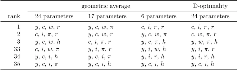
Table 1: Most informative and least informative sets of observables geometric average D-optimality rank 24 parameters 17 parameters 6 parameters 24 parameters
1 y,c, w,r y,c,w,π c,i,π,r c,i,π,r
2 c,i,π,r y,c,w,r y,c,w,π c,w,π,r
3 y,c, w,h c,i,π,r y,c,π,h y,w,π,h
33 c,i,w,π y,i, π,r y,i,w,h y,i,π,r
34 y,c, i,h y,c,i,π y,i,r,h y,i,r, h
35 y,c, i,π y,c,i,h y,c,i,h y,c,i,h
Note: The table shows the best 3 and the worst 3 sets of observables according to the geometric average and D-optimality criteria. The geometric average criterion is computed for 3 groups of parameters: 24 (all free) parameters; 17 (all except shock) parameters; 6 (onlyλ,ιp,ξp,σl,rπ,ry)
parameters.
relative importance to the researcher. An example of such a criterion is the weighted geometric average of the diagonal elements ofI−1(θ),
geometric average criterion =
k Y
i=1
CRLBwi
θi
!1/ Pk
i=1wi
(2.1)
whereCRLBθi is thei-th diagonal element ofI−1(θ),kis the number of free parameters, andwi is the
weight assigned toθi. The geometric average is more appropriate to use than the arithmetic average
since parameters typically have different range.
In what follows we use the finite sample FIM in order to take a proper account of the size of the sample, which is set to T=150, as in CFM.3We report three versions of the weighted geometric average
criterion with: (1) equal weights on all free parameters; (2) equal weights on the free structural param-eters and zero weights on the shock paramparam-eters; (3) equal weights on the six paramparam-eters emphasized in CFM, namelyλ,ιp,ξp,σl,rπ, andry, and zero weights on all other parameters. To be comparable
with CFM, we assume thatδ, λw and cg are known. This leaves 24 free parameters, 17 of which are
structural and the other 7 are shock parameters.
Table 1 lists the best three and worst three sets of variables according to each criterion. The set containing (c, i, π, r) is selected as most informative by two of the criteria, while the other two rank it among the top three sets. All criteria select sets containing (y, c, i) as least informative, with three of the criteria pickingh, and the fourth one selectingπ as the worst fourth variable. However, as can be seen in the first quadrant of Figure 1, the difference between (y, c, i, h) and (y, c, i, π), is very small, when the criterion is the geometric average of all 24 parameter. The figure shows the values associated with the 35 sets of variables, sorted from best to worst according to each criterion. It can be seen that (c, i, π, r) is in fact very close to the optimal sets selected by the first two criteria, which rank it second
3
and third, respectively. It also shows that there are numerically meaningful differences between the most and least informative sets of variables.
5 10 15 20 25 30 35
0.05 0.1 0.15 0.2 0.25
geometric average, 24 parameters
5 10 15 20 25 30 35
0.1 0.15 0.2 0.25 0.3 0.35 0.4
geometric average, 17 parameters
5 10 15 20 25 30 35
0 0.2 0.4 0.6 0.8 1
geometric average, 6 parameters
5 10 15 20 25 30 35
[image:6.595.146.466.176.378.2]-200 -180 -160 -140 -120 -100 D-optimality
Figure 1: Sorted values of different ranking criteria.
Table 2 reports the values of the individual CRLBs for the most and the least informative sets of variables, as per the results in table 1. In addition, the set (y, c, i, w) is also included as it was selected by CFM as one of the two most informative combinations. According to the criteria we use, this is the most informative combination of variables that includes simultaneously y, c, and i. It is ranked 9-th when the criterion is the geometric average of the CRLBs of the 17 structural parameters. As can be seen from the table, choosing one combination of variables over another usually involves a trade-off in terms of information about different parameters. Even the least informative set (y, c, i, h) is the most informative one, amongst those in the table, for three of the free parameters, ρga, ϕ, and σa. The
overall best set (c, i, π, r), yields the lowest (among the six in the table) CRLBs for a half of the free parameters, including three of the six deep parameters CFM focus on. If these are the parameters we are most interested in, the only reason to select (y, c, i, w) over (c, i, π, r) would be if one assigns much larger weights onσl andξp than on the other four parameters. In particular, there is much less
information about the Taylor rule parameters, due to the absence of bothr andπin that set. As can be seen from the last row in panel B, with equal weights (c, i, π, r) is more than twice as informative any of the sets that includey, c, andi.
One of the criteria used by CFM ranks the sets of variables on the basis of the sensitivity of the likelihood to a group of parameters of interest. The measures they use compare the scores of the non-singular and convoluted non-singular systems, and require simulated data to compute. A simpler and more direct measure of sensitivity to a single parameterθiis the expected curvature of log-likelihood function,
given by−E∂2ℓT(θ)
∂θ2 i
Table 2: Individual and overall parameter uncertainty
(c, i, π, r) (y, c, w, r) (y, c, w, π) (y, c, i, w) (y, c, i, π) (y, c, i, h) param. A. CRLBs of individual parameters
ρga 1.754 0.206 0.215 0.245 0.307 0.158
α 0.048 0.049 0.046 0.054 0.075 0.071
ψ 0.102 0.201 0.255 0.131 0.187 0.179
β 0.011 0.016 0.018 0.011 0.015 0.014
ϕ 2.812 3.852 4.874 6.153 6.770 2.566
σc 0.154 0.192 0.279 0.224 0.536 0.430
λ 0.031 0.027 0.035 0.044 0.099 0.151 Φ 0.323 0.123 0.124 0.159 1.482 0.221
ιw 0.180 0.269 0.072 0.243 1.061 1.359
ξw 0.142 0.021 0.018 0.021 0.177 0.257
ιp 0.044 0.247 0.074 0.208 0.099 1.187
ξp 0.155 0.044 0.043 0.048 0.401 0.480
σl 0.790 0.163 0.196 0.223 2.000 0.934
rπ 0.300 1.588 1.336 4.476 1.753 3.973
r△y 0.048 0.042 0.138 0.166 0.193 0.569
ry 0.060 0.296 0.236 0.632 0.257 1.057
ρ 0.028 0.050 0.053 0.082 0.091 0.189
ρa 0.015 0.018 0.022 0.025 0.029 0.023
ρg 0.004 0.011 0.014 0.014 0.015 0.016
ρI 0.049 0.064 0.074 0.095 0.100 0.066
σa 0.418 0.100 0.098 0.208 0.361 0.046
σg 0.145 0.044 0.048 0.043 0.089 0.054
σI 0.063 0.197 0.271 0.082 0.086 0.082
σr 0.016 0.017 0.132 0.126 0.255 0.292
B. Overall (geometric average of CRLBs)
24 parameters 0.094 0.092 0.103 0.126 0.218 0.217 17 parameters 0.133 0.129 0.126 0.170 0.321 0.384 6 parameters 0.120 0.169 0.138 0.256 0.391 0.834
C. Overall (D-optimality criterion)
24 parameters -183 -158 -148 -139 -114 -108
Note: Panel A shows the values of the Cram´er-Rao lower bounds (CRLBs) for sample sizeT = 150. Panel B shows the geometric averages of the bounds for three groups of parameters: 24 (all free) parameters; 17 (all except shock) parameters; 6 (onlyλ,ιp,ξp,σl,rπ,ry). Panel C shows the values of ln(det(I−1)). Lower values
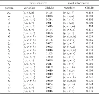
Table 3: Most sensitive and most informative sets of variables most sensitive most informative param. variables CRLBs variables CRLBs
ρga (y, c, i, h) 0.158 (y, c, i, h) 0.158
α (c, i, π, r) 0.048 (c, i, r, h) 0.039
ψ (c, w, π, r) 0.284 (c, i, π, r) 0.102
β (c, i, π, r) 0.011 (c, i, r, h) 0.009
ϕ (c, w, π, h) 2.679 (i, w, r, h) 1.793
σc (c, i, π, r) 0.154 (c, w, r, h) 0.131
λ (c, w, π, r) 0.028 (y, c, i, r) 0.022 Φ (y, w, π, h) 0.039 (y, w, π, h) 0.039
ιw (y, w, π, h) 0.106 (c, w, π, r) 0.065
ξw (y, w, π, h) 0.052 (y, c, w, h) 0.014
ιp (y, w, π, h) 0.042 (y, π, r, h) 0.036
ξp (y, w, π, h) 0.016 (y, w, π, h) 0.016
σl (y, w, π, h) 1.305 (y, c, w, r) 0.163
rπ (c, w, π, r) 1.282 (c, i, π, r) 0.300
r△y (c, i, π, r) 0.048 (y, c, w, r) 0.042
ry (c, w, π, r) 0.217 (c, i, π, r) 0.060
ρ (c, w, π, r) 0.032 (c, π, r, h) 0.026
ρa (c, w, π, r) 0.019 (c, i, w, r) 0.009
ρg (c, w, π, r) 0.012 (c, i, π, r) 0.004
ρI (c, w, π, r) 0.091 (c, w, π, h) 0.041
σa (y, w, π, h) 0.030 (y, w, π, h) 0.030
σg (y, i, w, r) 0.054 (y, c, i, w) 0.043
σI (c, i, π, r) 0.063 (c, i, π, r) 0.063
σr (c, i, π, r) 0.016 (c, i, π, r) 0.016
Note: The most sensitive set of variables w.r.t.θiis the one maximizing thei-th diagonal
element ofI. The most informative set is the one minimizing thei-th diagonal element ofI−1.
is not necessarily true. As can be seen in Table 3, the most sensitive and most informative sets coincide only for 6 of the 24 parameters. The table also shows the CRLBs corresponding the each set of variables. In several cases the differences are very large, meaning that the most sensitive selection contains much less information than the most informative one. A case in point is σl for which the CRLB with the
most sensitive combination (y, w, π, h) is 8 times larger than with the most informative combination (y, c, w, r).
As explained in greater details in Iskrev (2010), the values of the CRLBs are determined by the interactions of two factors – the sensitivity of the log-likelihood function to changes in individual parameters, and the degree of collinearity among the effects of such changes. A large value of the CRLB indicates that a parameter has only a weak effect on the log-likelihood function, and/or that its effect on the log-likelihood can to a large extent be offset by the effects of other parameters. In the case ofσl, it is much harder to distinguish its effect on the log-likelihood from the effects of parameters like
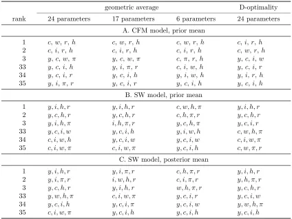
Table 4: Most informative and least informative sets of observables, different parameterizations geometric average D-optimality rank 24 parameters 17 parameters 6 parameters 24 parameters
A. CFM model, prior mean
1 c, w,r,h c,w,r,h c,w,r,h c, i,r,h
2 c, i,r,h c,i,r,h c,i,r,h c, w,r,h
3 y,c,w,π y,c,w,π c,π,r,h y,c, i,w
33 y,c,i,h y,i, π,r c,i,w,h y,c, i,r
34 y,c,i,r y,c,i,h y,i,w,h y,i,r, h
35 y,i,π,r y,c,i,r y,c,i,h y,c, i,h
B. SW model, prior mean
1 y, i, h, r y, i, h, r c, w, h, π y, i, h, r
2 y, c, h, r y, c, h, r c, h, π, r y, c, h, r
3 y, i, h, π i, h, π, r y, c, h, π y, c, i, r
33 y, c, i, w y, c, i, h y, i, w, h c, w, h, π
34 c, i, w, h y, c, i, w y, c, i, w c, i, w, π
35 c, i, w, π c, i, w, π y, c, i, h c, w, π, r
C. SW model, posterior mean
1 y, i, h, r y, i, π, r c, h, π, r y, i, h, r
2 y, i, π, r i, w, h, r c, i, π, r y, h, π, r
3 y, c, h, r y, i, h, r w, h, π, r y, c, h, r
33 y, w, h, π c, i, w, π y, c, i, r y, c, i, w
34 y, c, i, h y, c, i, π y, c, i, w y, w, h, π
35 c, i, w, π y, c, i, h y, c, i, h y, c, i, h
Note: see note to Table 1.
2.3
Are the results robust to changes in the parameter values and the
number of shocks?
The results presented in the last section are conditional on the particular parameter values and the assumptions CFM make regarding the number of shocks and the stationarity of the observables. Here we check whether the optimal selection of observables is robust to changes in the parameter values and the model specification.
Table 5: Optimal sets of observables, different parameterizations A. CFM model B. SW model
prior mean posterior mean prior mean posterior mean param. variables CRLBs variables CRLBs variables CRLBs variables CRLBs
ρga (y, i, w, h) 0.110 (y, c, i, h) 0.158 (y, c, i, h) 0.119 (y, c, i, h) 0.136
α (y, c, i, w) 0.005 (c, i, r, h) 0.039 (c, h, π, r) 0.025 (c, h, π, r) 0.167
ψ (y, c, i, w) 0.051 (c, i, π, r) 0.102 (c, i, h, r) 0.030 (y, c, i, r) 0.031
β (y, c, i, h) 0.003 (c, i, r, h) 0.009 (y, i, w, h) 0.148 (y, c, i, w) 0.251
ϕ (c, i, π, h) 0.076 (i, w, r, h) 1.793 (c, i, h, r) 0.667 (c, i, h, r) 2.544
σc (c, i, r, h) 0.039 (c, w, r, h) 0.131 (c, i, h, r) 0.202 (c, i, h, r) 0.253
λ (c, i, r, h) 0.004 (y, c, i, r) 0.022 (c, i, h, r) 0.047 (c, i, h, r) 0.079 Φ (y, w, π, h) 0.060 (y, w, π, h) 0.039 (c, i, w, h) 0.083 (y, i, h, r) 0.195
ιw (c, i, w, π) 0.083 (c, w, π, r) 0.065 (c, w, h, π) 0.122 (c, w, h, π) 0.173
ξw (y, w, π, r) 0.015 (y, c, w, h) 0.014 (c, w, h, π) 0.066 (c, w, h, r) 0.055
ιp (c, w, π, h) 0.044 (y, π, r, h) 0.036 (y, w, h, π) 0.073 (w, h, π, r) 0.093
ξp (y, w, π, h) 0.033 (y, w, π, h) 0.016 (y, w, h, π) 0.091 (y, w, h, π) 0.067
σl (c, w, r, h) 0.039 (y, c, w, r) 0.163 (c, w, h, π) 1.164 (c, w, h, r) 1.555
rπ (c, i, r, h) 0.167 (c, i, π, r) 0.300 (y, h, π, r) 0.552 (c, i, π, r) 0.510
r△y (c, w, r, h) 0.024 (y, c, w, r) 0.042 (y, i, π, r) 0.043 (c, i, h, r) 0.072
ry (c, i, r, h) 0.073 (c, i, π, r) 0.060 (c, h, π, r) 0.072 (c, i, π, r) 0.057
ρ (c, π, r, h) 0.021 (c, π, r, h) 0.026 (y, h, π, r) 0.068 (c, h, π, r) 0.047
ρa (c, i, r, h) 0.038 (c, i, w, r) 0.009 (y, i, w, h) 0.073 (y, i, h, r) 0.025
ρg (y, c, i, w) 0.052 (c, i, π, r) 0.004 (y, c, i, h) 0.076 (y, c, h, r) 0.017
ρI (c, i, r, h) 0.044 (c, w, π, h) 0.041 (c, i, h, r) 0.082 (c, i, h, r) 0.075
σa (y, i, w, h) 0.007 (y, w, π, h) 0.030 (y, i, w, h) 0.009 (y, i, w, h) 0.042
σg (y, w, π, r) 0.008 (y, c, i, w) 0.043 (y, c, i, h) 0.008 (y, c, i, h) 0.050
σI (c, i, r, h) 0.008 (c, i, π, r) 0.063 (c, i, h, r) 0.010 (c, i, w, r) 0.057
σr (c, π, r, h) 0.006 (c, i, π, r) 0.016 (c, h, π, r) 0.008 (c, h, π, r) 0.021
Note: see note to Table 3
are known.
Table 4 shows a summary of the results using the same criteria as before. Clearly, while there is considerable consistency in the ranking across different criteria, the optimal combination of variables is not invariant to the parametrization. Also, the two sets, (y, c, i, h) and (y, c, i, w), recommended by CFM, are consistently ranked among the least informative, especially when the focus is on the six deep parameters.
Table 6: Information gains, posterior mean of the SW model param. y c i w h π r
ρga 92 32 40 2 72 1 9
β 4 29 15 2 11 46 88
α 39 39 81 3 12 10 63
ψ 41 21 43 18 25 5 22
ϕ 4 30 54 6 22 5 28
σc 8 48 30 5 16 22 44
λ 13 39 29 8 25 10 45
Φ 26 16 33 9 77 6 15
ιw 2 3 3 84 2 55 5
ξw 7 31 12 34 16 14 22
ιp 4 3 3 38 7 60 6
ξp 30 9 21 58 65 36 9
σl 11 37 14 19 43 16 26
rπ 3 14 10 4 15 54 45
r△y 15 22 21 4 16 20 71
ry 4 12 8 5 17 50 43
ρ 3 13 8 4 15 53 56
ρa 32 38 37 8 39 3 31
ρg 43 57 36 4 21 3 23
ρI 2 14 63 3 8 5 13
σa 88 9 35 3 81 2 7
σg 90 53 56 3 37 1 11
σI 1 8 86 2 4 5 13
σr 3 11 1 1 17 38 89
Note: The efficiency gain EGθi(xj) measures the reduction in uncertainty about parameter
θidue to observing variablexj, expressed as a per cent of the parameter uncertainty when
2.4
The role of interest rate and inflation
One of the main conclusions reached by CFM is that neither interest rate nor inflation data should be selected, if one had to choose only four of the seven variables. This is surprising since some of the parameters CFM focus on are the price stickiness and price indexation parameters as well as the inflation and output coefficients in the monetary policy rule. Intuitively, one would expect that inflation and interest rate are very informative about these parameters.
To formally measure the amount of information contributed by each one of the observed variables, we compute parameter efficiency gains defined as the expected reduction in parameter uncertainty due to observing a variable, expressed as a percent of the uncertainty when that variable is not observed. Formally, the efficiency gain of a variablexj with respect to a parameterθi is defined as
EGθi(xj) = 100
CRLB
θi(x\xj)−CRLBθi(x)
CRLBθ
i(x\xj)
(2.2)
wherexis the set of all variables: x:={y, c, i, h, w, π, r}.
Since we want to know how much information each variable contributes relative to all other variables, we consider the full SW model, evaluated at the posterior mean value ofθ. Table 6 shows the efficiency
gains with respect to all free parameters. For 8 of them the largest efficiency gains come from either
r or π. This includes 4 of the 6 parameters CFM focus of, namelyιp, rπ,ry, for whichπ is the most
informative variable, andλ, for whichris the most informative variable. As can be seen from the table,
πandrare also very informative about several other parameters, e.g. α,σc,ιw,ξp, andσl, suggesting
that excluding these variables would lead to a substantial loss of information.
2.5
Monte Carlo study
The FIM-based analysis is a simple way of quantifying the information content of the restrictions the DSGE model imposes on the joint probability distribution of the observed variables. This makes it well suited for ranking different sets of observables in terms of the amount of information about the unknown parameters one couldexpect to get from each set. In this section we evaluate the predictions of the FIM approach using Monte Carlo simulations. In particular, we simulate the baseline model with 4 structural shocks to generate 400 artificial samples of 150 observations for each of the seven observable variables. We estimate by maximum likelihood the 24 free parameters using different subsets of four variables. We focus on the six subsets presented in Table 2, which comprise of the most informative ones according to our FIM-based criteria, and the subsets recommended by CFM.
Table 7: Simulated root mean squared errors,T = 150
(c, i, π, r) (y, c, w, r) (y, c, w, π) (y, c, i, w) (y, c, i, π) (y, c, i, h) param. A. individual parameters
ρga 0.478 0.216 0.219 0.229 0.275 0.173
α 0.050 0.053 0.060 0.050 0.060 0.055
ψ 0.110 0.204 0.251 0.148 0.195 0.187
β 0.011 0.016 0.020 0.011 0.015 0.012
ϕ 3.120 3.321 3.230 3.849 4.222 3.256
σc 0.135 0.214 0.359 0.306 0.405 0.447
λ 0.028 0.034 0.059 0.069 0.098 0.097 Φ 0.389 0.144 0.181 0.209 0.690 0.267
ιw 0.244 0.299 0.086 0.295 0.418 0.428
ξw 0.072 0.029 0.021 0.033 0.221 0.250
ιp 0.050 0.242 0.078 0.236 0.128 0.450
ξp 0.112 0.058 0.058 0.073 0.205 0.283
σl 1.186 0.288 0.315 0.347 3.529 2.226
rπ 0.394 0.803 0.816 0.914 0.735 0.824
r△y 0.053 0.046 0.151 0.218 0.152 0.395
ry 0.073 0.224 0.230 0.245 0.177 0.161
ρ 0.025 0.044 0.054 0.117 0.083 0.121
ρa 0.008 0.017 0.051 0.052 0.062 0.040
ρg 0.005 0.012 0.059 0.026 0.031 0.030
ρI 0.049 0.060 0.066 0.070 0.082 0.070
σa 0.148 0.096 0.144 0.258 0.241 0.057
σg 0.164 0.047 0.064 0.047 0.077 0.056
σI 0.058 0.268 0.301 0.114 0.130 0.100
σr 0.017 0.018 0.131 0.145 0.182 0.181
B. Overall
24 parameters 0.085 0.097 0.125 0.137 0.191 0.176 17 parameters 0.112 0.128 0.142 0.162 0.252 0.237 6 parameters 0.132 0.171 0.158 0.212 0.325 0.392
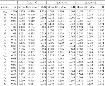
Table 8: Monte Carlo results and theoretical CRLBs (part I) (c, i, π, r) (y, c, w, r) (y, c, w, π) param. True Mean Std. dev. CRLB Mean Std. dev. CRLB Mean Std. dev. CRLB
ρga 0.510 0.459 0.476 1.754 0.503 0.216 0.206 0.452 0.211 0.215
α 0.20 0.210 0.049 0.048 0.204 0.053 0.049 0.216 0.058 0.046
ψ 0.26 0.258 0.110 0.102 0.272 0.203 0.201 0.277 0.250 0.255
β 0.99 0.988 0.010 0.011 0.983 0.014 0.016 0.980 0.017 0.018
ϕ 5.48 6.033 3.074 2.812 5.113 3.305 3.852 4.601 3.111 4.874
σc 1.39 1.408 0.134 0.154 1.477 0.196 0.192 1.524 0.334 0.279
λ 0.71 0.705 0.028 0.031 0.696 0.031 0.027 0.687 0.054 0.035 Φ 1.61 1.681 0.383 0.323 1.652 0.138 0.123 1.530 0.162 0.124
ιw 0.59 0.592 0.244 0.180 0.698 0.279 0.269 0.560 0.080 0.072
ξw 0.73 0.734 0.072 0.142 0.716 0.026 0.021 0.729 0.021 0.018
ιp 0.47 0.456 0.048 0.044 0.506 0.239 0.247 0.463 0.078 0.074
ξp 0.65 0.615 0.107 0.155 0.640 0.057 0.044 0.659 0.057 0.043
σl 1.92 2.235 1.145 0.790 1.969 0.285 0.163 1.933 0.315 0.196
rπ 2.03 2.129 0.382 0.300 1.907 0.794 1.588 2.155 0.808 1.336
r△y 0.22 0.239 0.049 0.048 0.213 0.046 0.042 0.263 0.144 0.138
ry 0.08 0.092 0.072 0.060 0.211 0.182 0.296 0.218 0.184 0.236
ρ 0.87 0.871 0.025 0.028 0.874 0.044 0.050 0.883 0.052 0.053
ρa 0.95 0.947 0.007 0.015 0.948 0.017 0.018 0.923 0.043 0.022
ρg 0.97 0.968 0.004 0.004 0.968 0.012 0.011 0.949 0.055 0.014
ρI 0.71 0.708 0.049 0.049 0.712 0.060 0.064 0.720 0.066 0.074
σa 0.46 0.421 0.143 0.418 0.442 0.095 0.100 0.504 0.137 0.098
σg 0.61 0.619 0.164 0.145 0.605 0.046 0.044 0.598 0.063 0.048
σI 0.60 0.609 0.058 0.063 0.758 0.216 0.197 0.810 0.216 0.271
σr 0.25 0.254 0.017 0.016 0.249 0.018 0.017 0.276 0.129 0.132
Note: The means and standard deviations of MLE are calculated using 400 Monte Carlo simulations.
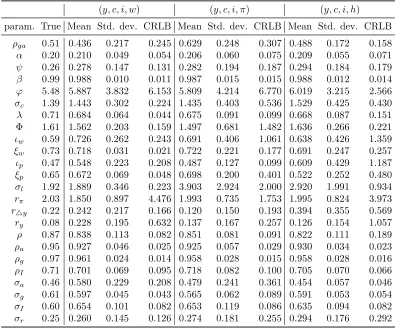
the values of the RMSE are generally very similar to the respective values of the CRLBs. This is not something we would necessarily expect for at least two reasons. First, the CRLBs are by definition lower bounds on the standard deviations of unbiased estimators. Hence, even if the estimation bias is small, the actual RMSEs may be significantly larger than the theoretical lower bounds. Second, the CRLBs do not account for any a priori restrictions on the parameter values, such as the restriction that a parameter has to be between 0 and 1. In our ML estimation we imposed such restrictions on a number of parameters, e.g. β, α, λ, ξw, ξp, ιw, ιp, as well as the autoregressive coefficients of the shocks.4
One consequence of ignoring these restrictions could be that the theoretical bounds on the estimation uncertainty are larger than the actual uncertainty. Such discrepancies occurred in a very few cases in our simulations, as can be seen in Tables 8 and 9 (see for instance the values forρgawhen (c, i, π, r) is
observed). In the vast majority of cases the theoretical bounds are very close to the simulation-based standard errors.
4
Table 9: Monte Carlo results and theoretical CRLBs (part II) (y, c, i, w) (y, c, i, π) (y, c, i, h) param. True Mean Std. dev. CRLB Mean Std. dev. CRLB Mean Std. dev. CRLB
ρga 0.51 0.436 0.217 0.245 0.629 0.248 0.307 0.488 0.172 0.158
α 0.20 0.210 0.049 0.054 0.206 0.060 0.075 0.209 0.055 0.071
ψ 0.26 0.278 0.147 0.131 0.282 0.194 0.187 0.294 0.184 0.179
β 0.99 0.988 0.010 0.011 0.987 0.015 0.015 0.988 0.012 0.014
ϕ 5.48 5.887 3.832 6.153 5.809 4.214 6.770 6.019 3.215 2.566
σc 1.39 1.443 0.302 0.224 1.435 0.403 0.536 1.529 0.425 0.430
λ 0.71 0.684 0.064 0.044 0.675 0.091 0.099 0.668 0.087 0.151 Φ 1.61 1.562 0.203 0.159 1.497 0.681 1.482 1.636 0.266 0.221
ιw 0.59 0.726 0.262 0.243 0.691 0.406 1.061 0.638 0.426 1.359
ξw 0.73 0.718 0.031 0.021 0.722 0.221 0.177 0.691 0.247 0.257
ιp 0.47 0.548 0.223 0.208 0.487 0.127 0.099 0.609 0.429 1.187
ξp 0.65 0.672 0.069 0.048 0.698 0.200 0.401 0.522 0.252 0.480
σl 1.92 1.889 0.346 0.223 3.903 2.924 2.000 2.920 1.991 0.934
rπ 2.03 1.850 0.897 4.476 1.993 0.735 1.753 1.995 0.824 3.973
r△y 0.22 0.242 0.217 0.166 0.120 0.150 0.193 0.394 0.355 0.569
ry 0.08 0.228 0.195 0.632 0.137 0.167 0.257 0.126 0.154 1.057
ρ 0.87 0.838 0.113 0.082 0.851 0.081 0.091 0.822 0.111 0.189
ρa 0.95 0.927 0.046 0.025 0.925 0.057 0.029 0.930 0.034 0.023
ρg 0.97 0.961 0.024 0.014 0.958 0.028 0.015 0.958 0.028 0.016
ρI 0.71 0.701 0.069 0.095 0.718 0.082 0.100 0.705 0.070 0.066
σa 0.46 0.580 0.229 0.208 0.479 0.241 0.361 0.454 0.057 0.046
σg 0.61 0.597 0.045 0.043 0.565 0.062 0.089 0.591 0.053 0.054
σI 0.60 0.654 0.101 0.082 0.653 0.119 0.086 0.635 0.094 0.082
σr 0.25 0.260 0.145 0.126 0.274 0.181 0.255 0.294 0.176 0.292
3
Concluding remarks
Our results can be summarized as follows: (1) The rank condition for identification is not informative about the optimal choice of observables for the model that was analyzed. In general, such a criterion could be useful when only one, or a very few, of the many possible sets of variables satisfy the identifi-cation condition. This seems to rarely be the case in practice. (2) At the baseline parametrization of the model the most informative set of variables includes consumption, investment, interest rate, and inflation. (3) The most informative set of variables is not invariant to the parametrization of the model or the number of shocks.
References
Bierens, H. J.(2007): “Econometric analysis of linearized singular dynamic stochastic general equi-librium models,” Journal of Econometrics, 136, 595–627.
Canova, F., F. Ferroni, and C. Matthes (2014): “Choosing the variables to estimate singular DSGE models,”Journal of Applied Econometrics, 29, 1099–1117.
Iskrev, N.(2010): “Evaluating the strength of identification in DSGE models. An a priori approach,” Working paper series, Banco de Portugal.
Rothenberg, T. J. (1971): “Identification in Parametric Models,”Econometrica, 39, 577–91, avail-able at http://ideas.repec.org/a/ecm/emetrp/v39y1971i3p577-91.html.